Comparative Analysis of Classifiers for Classification of Emergency Braking of Road Motor Vehicles


Graduate School of Science and Engineering, Doshisha University, Kyoto 602-8580, Japan
*
Author to whom correspondence should be addressed.
Algorithms 2017, 10(4), 129; https://doi.org/10.3390/a10040129
Submission received: 30 September 2017
/
Revised: 12 November 2017
/
Accepted: 17 November 2017
/
Published: 22 November 2017
(This article belongs to the Special Issue Computational Intelligence and Nature-Inspired Algorithms for Real-World Data Analytics and Pattern Recognition)
Abstract
:We investigate the feasibility of classifying (inferring) the emergency braking situations in road vehicles from the motion pattern of the accelerator pedal. We trained and compared several classifiers and employed genetic algorithms to tune their associated hyperparameters. Using offline time series data of the dynamics of the accelerator pedal as the test set, the experimental results suggest that the evolved classifiers detect the emergency braking situation with at least 93% accuracy. The best performing classifier could be integrated into the agent that perceives the dynamics of the accelerator pedal in real time and—if emergency braking is detected—acts by applying full brakes well before the driver would have been able to apply them.
1. Introduction
In recent years, there has been noticeable progress in technologies devoted to driving aids in road motor vehicles [1]. The interest in this field is driven by the continuous desire to increase road safety. There are two main types of driving aids: passive and active. Passive driving aids simply notify the driver about the detected improper condition of the car (e.g., low tire pressure, low hydraulic brake pressure, elevated temperature of the coolant of the engine, etc.), driver (sleepiness, fatigue, distraction), road (possibility of ice, wet conditions), or even dangerous traffic situations (unintended lane crossing, presence of objects in the blind spots of the driver’s vision, etc.). On the other hand, active driving braking aids are even able to revoke the inputs of the human driver and delegate control to itself if an imminent traffic accident has been anticipated or if the driver loses the control of the car. Examples of active driving aids include anti-locking brake systems, traction control, an electronic stability program, and automated brake assistance. The latter can be implemented either as a fully automated braking system [2,3] or as an assistant to the human driver [4,5]. Automated braking aids are meant to be rather helpful; however, the current realization of these systems faces many engineering and psychological challenges. Among them is the recognition that fully automated driving aids seldom result in safer driving due to the inflated sense of safety of human drivers (according to the risk homeostasis theory [6]). With the intention of building a reliable and easily applicable helpful system, we decided to leave fully automated braking aids out of the scope of our current research and focus on brake assistance instead.
The modern research on brake-assisting typically considers the brain and the myoelectric activities measured by electroencephalography (EEG) and electromyography (EMG), respectively [7,8,9]. These approaches demonstrate the high feasibility of predicting the emergency situation on the road. However, while EMG measurements are reliable, the brain waves that are recorded by EEG cannot be considered as a credible signal because it is usually affected by the variety of circumstances that dynamically (and, usually, unpredictably) arise while driving. For example, an eventual unsteady directional motion of the vehicle or even simple movements of the head or body of the driver could significantly alter the obtained signals. Moreover, as the researcher investigating these approaches acknowledges, the interference of simple actions such as chewing, raising eyebrows, or eye blinking will be prevalent in real driving. Also, we would like to emphasize both the inconvenience and questionable practical applicability of these approaches: the contemporary implementations of mobile EEG and EMG do not allow for convenient, easy, or quick setup.
In another study [10], the authors built a framework that allows for the assessment of both the degree of criticality of the current road traffic situation and the need for intervention by an intelligent driving system. The proposed framework is based on the processing of several parameters obtained from the sensors of the vehicle via the controller area network (CAN). These parameters include the displacement time of the driver’s foot (e.g., the time needed to move the foot from the accelerator pedal to the brake pedal), and head and facial movements. An alternative approach [11] takes into account the speed of releasing the accelerator pedal, foot displacement, and the speed of the brake pedal in order to detect emergency braking situations. The current industrial systems, however, from the whole set of parameters that could, in principle, characterize the behavior of the driver during emergency braking situations, consider only the motion pattern of the pressed brake pedal [12]. These systems are intended to support drivers who apply the brake pedal quickly but not strongly enough by applying the maximum force to the brakes in emergency situations. The behavior of the driver in such emergency braking situations was extensively explored in [13]. In the latter studies, the authors also proposed both a brake-force-based and a speech-based approach for identifying hazardous situations on the roads.
Without any doubt, in cases of emergency braking, the aforementioned approaches are able to reduce the driver’s response time and, as a consequence, the braking distance of the car. In none of these studies, however, was the motion pattern of the (lifting) accelerator pedal considered as the sole information needed for the reliable detection of the emergency braking situations.
These facts motivated us to investigate the feasibility of predicting the emergency braking situation even before the driver presses the brake pedal (as implemented by most of the current industrial brake assistant systems)—namely, from the pattern of lifting the accelerator pedal [14]. In the case of detecting the special pattern—pertinent to the emergency braking situation—of the motion of accelerator pedal, the proposed system should be able to automatically activate the brakes well before the driver would have been able to apply them. As shown in Figure 1, different driving situations—such as accelerating, cruising, slowing down, normal braking, and emergency braking—exhibit different, specific motion of the accelerator pedal. We obtained the data illustrated in Figure 1 from the modelled parametric data recorder of a car driven by a sample human driver in a full-scale Forum-8 drive simulator [15], as shown in Figure 2. The simulator realistically models a real-world car featuring an automatic transmission, which implies that the driver lifts the accelerator pedal (Figure 1c–e) only when they really intend to reduce the speed of the car (or, ultimately, to stop it). Apparently, just before the driver applies the emergency brake, they abruptly lift the accelerator, and the latter quickly returns to its original position [11,16], as illustrated in detail in Figure 3.
In principle, it might be possible to predict the emergency braking situation solely by considering the dynamics of the accelerator pedal. By saying “to predict” we actually mean to classify the current driver’s intention: whether they are going to apply emergency brakes or just normally decelerate the car. A straightforward approach for classification of driver’s intention could be based on a comparison of the rate of change of the position of accelerator with a predefined threshold. Exceeding the threshold would be associated with an urgency of the driving situation, and, consequently, with the intention of the driver to apply emergency braking soon. This assumption is based on the fact that the driver lifts their foot faster than the speed at which the pedal returns to its neutral position. In such a situation, the latter will, indeed, return to its initial position without being hindered by the moving foot of the driver. The motion pattern of the unhindered accelerator pedal could be established analytically from its (known) mechanical characteristics—mass, moment of inertia, friction, displacement of the return spring, and its constant. However, the results of preliminary experiments suggest that such a threshold criterion could not be applied straightforwardly to every driver due to the natural variations in the patterns of the drivers lifting their foot from the accelerator.
The main objective of our research is to resolve the problem of emergency braking classification (EBC) solely from the motion pattern of the accelerator pedal by building an intelligent classifier. We also intend to verify the robustness and generality of the proposed solution to the EBC problem on the data of drivers who have not participated in the process of training the classifiers. In addition, we shall integrate and test the classifier as a brake assisting aid in the full-scale driving simulator that we initially used to collect the training data. The key motivation of our research is in the opportunity of reducing the time lag between two instants: when the driver moves their foot from the accelerator pedal (Figure 3a) and the moment when they press the brake pedal to its maximum position (Figure 3c). In properly classified cases, the proposed brake assisting system would be able to activate the brakes automatically and, as a consequence, to reduce the above-mentioned time lag.
2. Methods
Apart from building the real-time braking assistance, in our research we also intend to compare the alternative classification approaches and to optimize the values of their respective parameters.
2.1. Quality Metrics
In order to evaluate the performance and quality of the trained classifier, applied to the particular EBC problem, we consider using metrics which are not commonly considered. The straightforward approach would have been to use the percentage of correct answers—accuracy. However, this metric if not feasible for the considered EBC problem because if the classifier detects all normal driving cases and ¼ of emergency braking cases, then the accuracy will be equal to 0.7. However, we will miss almost all emergency braking events, suggesting that the metric is not adequate for the evaluation of quality of the classifiers. Therefore, in our approach we apply more informative metrics like precision, recall, and F-score [17] to evaluate the performance of the classifier. For illustration of these metrics, we shall consider the confusion matrix as shown in Table 1. The table illustrates four categories and provides information about how many times the classifier has given the correct answer and how many times the wrong decision has been adopted.
The true positive category (TP) is equal to the number of samples which are classified as class “1” (emergency braking) and are actually in the class “1”. False positive (FP) corresponds to the samples for which the correct class is “0” (normal driving) but the classifier returns “1”; vice versa, if the classifier recognizes the sample as “0” but the real answer is “1”, then the sample is considered as a false negative (FN). Finally, true negative (TN) corresponds to the cases when the sample belongs to the class “0” and the classifier indeed returns “0”. In this way, recall and precision can be expressed as follows:
Both of these metrics describe different aspects of the classifier: the higher the precision, the lower the FP; and the higher the recall, the lower the FN. Obviously, FP (resulting in emergency braking during normal driving conditions) cases are not preferable due to the resulting uncomfortable driving (and, in some cases, unsafe). However, FP should not necessarily be considered dangerous; we shall elaborate as to why later, in the discussions section of this article. Therefore, for the sake of the comfort of the driver (and passengers) we are interested in maximizing the precision metric. On the other hand, it is necessary to detect as many cases of emergency braking as possible and, as a consequence, to outperform the straightforward threshold classifier which apparently features relatively low values of recall. Thereby, we should pay attention to both of these metrics, and the F-score allows us to do this objective:
The F-score can be seen as the harmonic mean of both precision and recall. The scaling coefficient 2 is used in order to normalize the value of the F-score to 1 when both recall and precision are equal to 1.
2.2. Cross-Validation
Cross-validation (CV) [18] is a method of evaluating the model (in the considered case: the classifier of emergency braking situations) and its behavior on independent data. When evaluating the classifier, the available dataset is divided into k subsets (folds). Then, the model is trained on k − 1 folds and the rest of data is used for validation. The procedure is repeated k times. As a result, each of the k folds is used for testing. By averaging the validation quality as illustrated in Figure 4, we obtain the value of the final quality—CV score—of the chosen model with the most even use of the available data. Calculating the CV score is computationally expensive. However, at the same time, it is rather parsimonious in terms of the required amount of data. In addition, it is proven to be able to prevent overfitting of classifiers to a particular set of training data [19].
2.3. Threshold Classifier
The threshold classifier is a one-dimensional classifier which determines the class affiliation of the sample by comparing its value to the predetermined threshold. In our work, we use the threshold classifier as a benchmark. In the Methodology section, we describe the building process of this classifier.
2.4. K-Nearest Neighbors
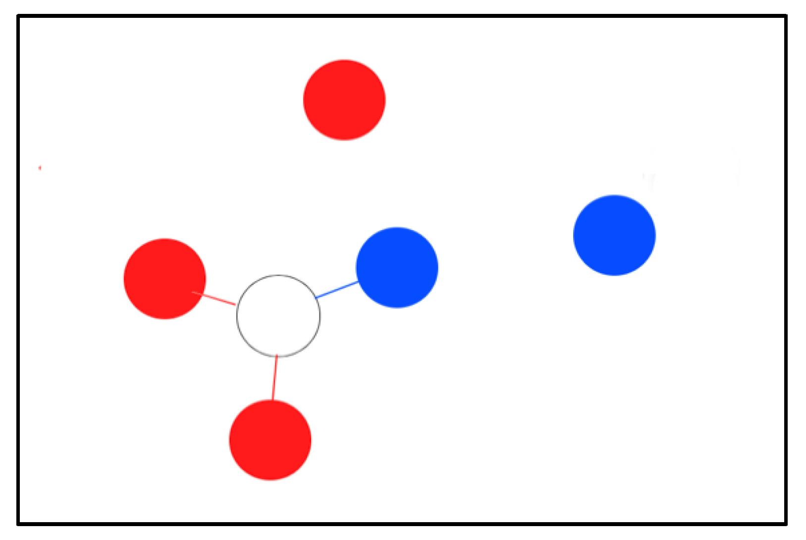
K-nearest-neighbors-based (k-NN) [20] classification is a type of non-generalizing learning; this means that the method doesn’t build a general model with an eye to classify the sample, but simply stores the whole dataset. The classifier makes a decision by the majority voting of the k nearest neighbors of each sample. A testing sample is assigned the class which has the most significant number of representatives within the nearest neighbors of the sample. For the example, shown in Figure 5, the white sample will be assigned the red class when k is equal to 3.
2.5. Support Vector Machine
Another classification method which is being used in the considered classification problem is the support vector machine (SVM) [21]. This method performs well in many linear and non-linear problems; it is also able to process high-dimensional and large data sets.
The basic idea of SVM is building a hyperplane which splits the training set into the necessary number of classes (in our case, two). When the hyperplane is built, a testing sample is placed on the plane. Depending on its position relative to the hyperplane, we infer the class affiliation of the testing sample.
Formally, the problem can be formulated as follows: begin with a training set of N points (xi, yi), where xi ∈ and yi ∈ are the i-th input and output samples, respectively. SVM constructs a classifier, which can be represented by a function:
where xk are support vectors, αi are positive real numbers, while b (bias) is a real number. The kernel K can be used in various forms: (linear kernel), (polynomial kernel of degree n), , or (sigmoid kernel), where kernel parameters and are real constants.
The learning of SVM lies in finding f(x), which minimizes the following objective:
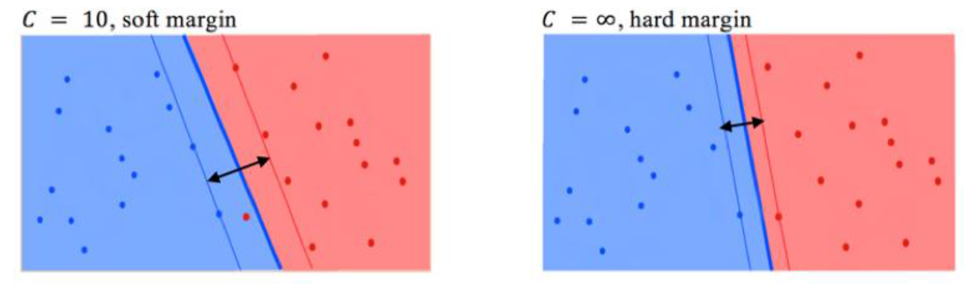
where the first term l is a loss function, if , and the second term Ω is a penalty function of our model parameters. The parameter C specifies the desire of avoiding the misclassification of each training sample. For example, a large value of C will reduce the width of the hyperplane margin, which will potentially cause fewer errors on the training set. At the same time, a low C will widen the hyperplane margin, as shown in Figure 6.
2.6. Extreme Gradient Boosting
The last method which is considered in our work is Extreme gradient boosting (XGBoost) [22]. XGBoost is a scalable machine learning approach which has proved to be successful in many machine learning and data mining challenges [23,24]. Essentially, XGBoost is an ensemble of K classification and regression trees (CART) [25]. Unlike decision trees, CART assign a real score to each leaf (outcome or target). The final score of y (output) is a sum of K additive functions as follows:
where fk corresponds to independent tree structure and leaf weights, while xi is a testing object. F represents a testing space of all CART. For learning the set of functions, the following objective is used:
The first term is a differentiable loss function, l, which calculates the difference between the target and the predicted . Ω is a regularization term which prevents over-fitting by penalizing the complexity of the model. Parameters T and w correspond to the number of leaf nodes and the weight of each of them, respectively. Parameters γ and λ are constants which control the degree of regularization.
The ensemble tree model includes functions as parameters and cannot be optimized within traditional methods in Euclidian space; therefore, we employed the following additive approach for its training: assuming that at the tth iteration we have a prediction of the ith instance, we add ft(xi) to our objective function.
In order to quickly optimize the general setting of this objective, the second-order approximation is used:
Because the loss function is calculated at the current time step t, we can easily remove it:
By defining Ij = {i|q(xi) = j} as an instance set of leaf j for a given tree structure q(x), the objective function can be rewritten as follows:
For a fixed structure q(x), the optimal weight wj of leaf j will be
while the corresponding optimal value will be
Finally, in order to score a leaf node during splitting, we use the following expression:
Here IL and IR are the instance sets of the left and right nodes after the split, I = IL ∪ IR, and is the regularization on the additional leaves. It is important to note that—besides the regularization technique—shrinkage and feature subsampling are also used in XGBoost [22].
2.7. Genetic Algorithms
GA are nature-inspired searching algorithms initially proposed by Holland [26]. GA are widely used in various design, control, and optimization problems when exact analytical approaches either do not exist or are too time-consuming to be applied. Moreover, GA [27,28] can be used for solving problems that feature an unknown, non-uniform, discontinuous, or intractably large search space. The representation of the candidate solution in GA is in the form of a population of linear strings (i.e., chromosome) of evolving values of parameters (genetic alleles). Mathematically, the chromosome could be represented as an n-dimensional vector (x1, x2, …, xn) where each coordinate xi of the vector—the value of a parameter to be optimized—represents a genetic allele. The objective of applying GA is to find such a chromosome that results in an optimal value of a given target—fitness function F. It is important to note that the design of fitness function F is domain-specific, and depends on the nature of the problem being solved. In GA, the quest for the best chromosome (solution), i.e., the chromosome that yields an optimal value of F, consists of the following main steps:
- Step 0
- Creating the initial population of randomly generated chromosomes;
- Step 1
- Evaluating the fitness of chromosomes in the population;
- Step 2
- Checking the termination criteria: good enough fitness value (of the best chromosome in the population), too long runtime, or too many generations. GA terminates if one of the criteria is satisfied;
- Step 3
- Selection: selecting the mating pool of chromosomes. The size of the mating pool is a fraction (i.e., 10%) of the overall size of the population, and the selection of the chromosomes in the mating pool is fitness-proportional (roulette-wheel, tournament, elitism, etc.);
- Step 4
- Reproduction: implementing crossover by swapping random fragments of randomly selected pairs (parents) of chromosomes from the mating pool. Crossover produces pairs of offspring chromosomes that are inserted into the newly growing population; and
- Step 5
- Mutation: random gene(s) of newly generated offspring chromosomes are randomly modified with a given probability.
The implementation of GA could be illustrated by the following pseudo-code:
  Generate initial population;
  Evaluate population;
  While not (Termination Criteria) do
  Selection; // Creating the mating pool of surviving chromosomes
  Reproduction; // Crossing over a randomly selected pair of survived
  chromosomes
  Mutation; // Mutating the newly produced (by crossover) offspring
  Evaluate population;
3. Proposals
Achieving our objective of building a learned EBC implies that our research should be implemented in the following five consecutive stages: (i) acquiring and analyzing the data on the dynamics of the accelerator and brake pedals of a car simulated in a full-scale drive simulator; (ii) exploring the straightforward techniques for EBC; (iii) adopting machine learning methods for EBC; (iv) evaluating the proposed classifier on unforeseen data; and, finally, (v) integrating EBC in the full-scale drive simulator in order to verify its performance in a real-time setting and to evaluate the feedback from the drivers.
4. Methodology
4.1. Acquiring Data
In order to acquire the time series data of the dynamics of the accelerator pedal, we asked 12 drivers (men and women, aged 22–52) to drive a simulated car in a full-scale Forum-8 driving simulator [15] in various traffic situations and road conditions. The main requirement for drivers was the possession of a driving license. The details of experimental tracks are shown in Table 2.
For the sake of separating the data samples into two categories—normal driving and emergency braking, respectively—we conducted two series of experiments, as elaborated in Table 3.
During the experiment on normal driving, the drivers were asked to drive a car in a normal way which actually implies that they were not allowed to apply emergency braking. In the emergency braking experiments, each of the drivers was audibly signaled to stop the car suddenly, even though there was no real danger on the simulated road. When the driver heard the specific signal, they were supposed to apply the brake pedal to its maximum as soon as possible. With the intention of maintaining complete separation of the data samples belonging to the two classes (normal driving and emergency braking, respectively), the drivers were asked not to use normal brakes during the second series of experiments. However, they were allowed to decelerate the car by means of lifting the accelerator pedal only. The modeled parametric data recorder logged all the relevant time series for future offline analysis. The acquired raw time series were a sequence of positioning of both pedals (within the range 0–100) sampled with a frequency of 25 Hz. This is the maximum sampling frequency allowed by the adopted drive simulator. During the processing of the mentioned time series, we could extract 1304 events in total, including both normal driving (class “0”) and emergency braking (class “1”) events.
4.2. Data Analysis and Feature Extraction
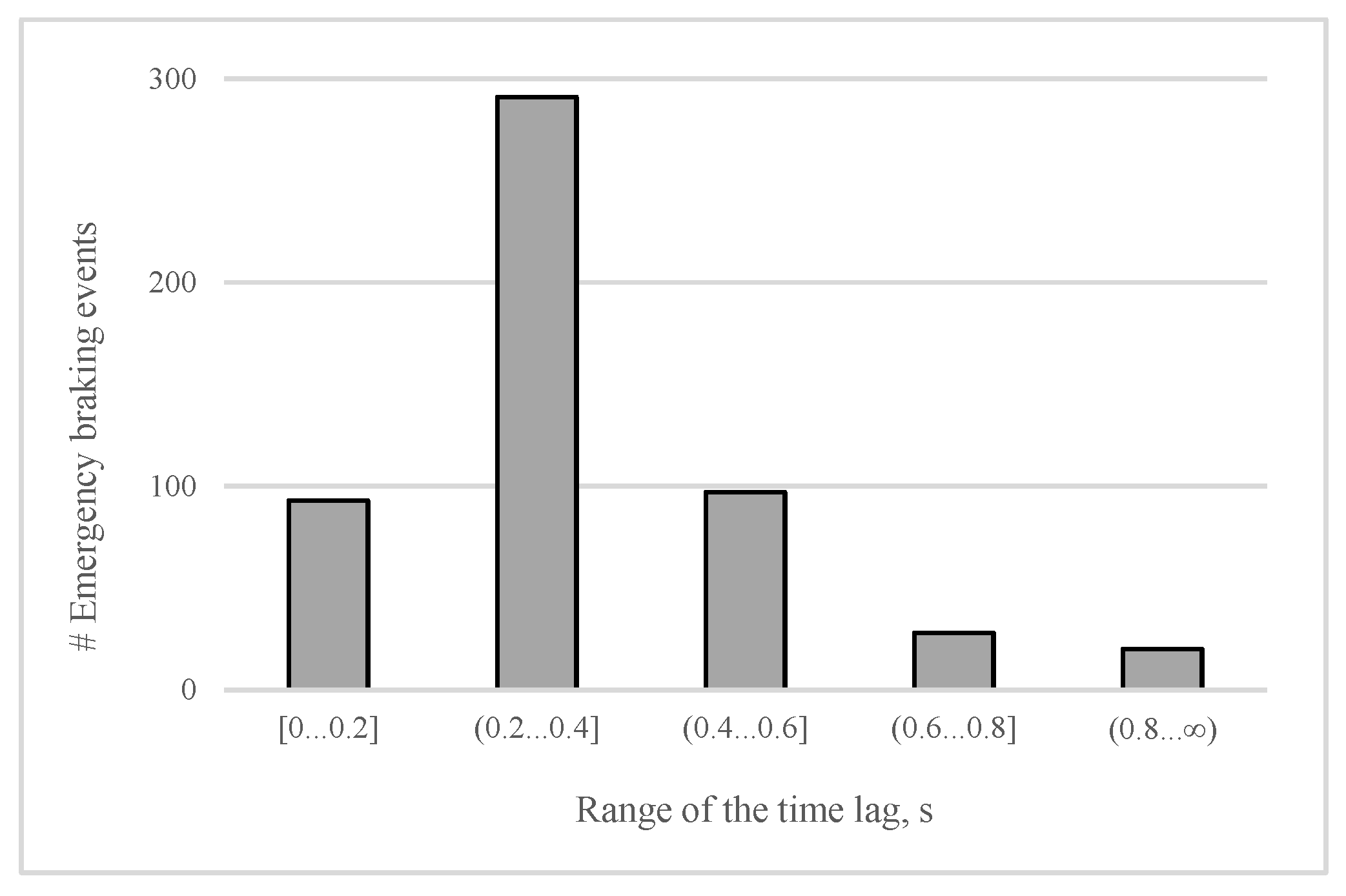
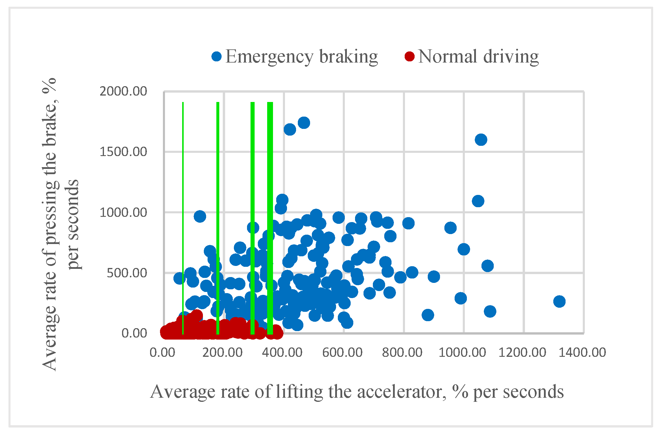
First, we shall analyze the distribution of the time lag between lifting the accelerator and pressing the brake pedal completely (emergency cases) among all testers. The importance of the distribution is that it allows us to estimate the average time that the proposed brake assisting system could save. As illustrated in Figure 7, in most (55%) of the emergency braking events, the time lag covers the interval (0.2 s, 0.4 s]. For the car moving at a speed of 50 km/h, this time lag matches to a traveled distance of between 2.8 m and 5.6 m. Furthermore, a time lag of 0.4 s or higher is registered in about 27% of the emergency braking cases, suggesting that, in more than half of cases at the speed of 50 km/h, the corresponding traveled distance can be even longer than 5.6 m. Consequently, in more than half of the cases of emergency braking, an eventual automated application of brakes would be able to reduce the overall stopping distance, remarkably, by at least 5.6 m (when the driving speed is 50 km/h). As well as measuring the time lag for all drivers, we also extracted several key features of both pedals. Among them are the highest position of the accelerator pedal before starting the deceleration (mP), the maximum and average rate of lifting the accelerator (mR and aR respectively), the maximum and the average rate of pressing the brake pedal, and the maximum position of the pressed brake pedal. The average rate is the pedal speed on the interval where the pedal position is decreasing or increasing (in the case of applying brakes). The maximum rate value is the maximum pedal speed among 0.04 s periods of the mentioned interval.
According to our assumption, it could be possible to classify the driver’s intention to apply emergency braking if the value of mR or aR is higher than a certain threshold. As Figure 8 and Figure 9 illustrate, higher rates of pressing the brake pedal correspond to emergency braking situations and often come before the swift release of the accelerator pedal. Consequently, some of the samples belonging to the same class are very close to each other.
4.3. Building Classifiers
Before proceeding with the training of classifiers, we assigned the time series data obtained from 10 sample drivers to the training set and the data of 4 other drivers to the testing set. This approach of separating the data allows good generalization for the classifier. Eventually, the number of samples in the training and testing sets are 1044 and 260 respectively: for the training set there are 447 samples of class “1” and 597 of class “0”, while in the testing set, these numbers are 82 and 178, respectively.
In order to build an eventual threshold classifier, we gradually “move” the threshold for both mR and aR until the classifier ceases to misclassify the samples from class “1” in the training set. In this way, the threshold for mR was found to be 894, and that for aR was found to be 411, as shown in Figure 10.
Despite its simplicity, the threshold classifier is able, indeed, to detect some of the emergency braking cases from the testing set (see Results). However, we presume that a combination of features (rather than single ones) pertinent to the dynamics of the accelerator pedal would be needed for successful classification of emergency braking. Therefore, we investigate the feasibility of solving the EBC problem by applying more intelligent approaches based on machine learning.
In order to employ SVM and k-NN for the emergency brake classification, we use a powerful machine learning library for the Python programming language: scikit-learn [29]. Besides providing an enormous amount of various machine learning methods with its friendly APIs [30], scikit-learn allows us to visualize the dataset in a very representative way. To employ gradient-boosted trees in our work, we used an open source package of XGBoost [31] which supports multiple programming languages including C++, Python, R, Java, Scala, and Julia.
It is important to note that, for using k-NN and SVM, we applied a standardization procedure to the dataset since this is a common requirement for these methods. This procedure standardizes features by removing the mean and scaling to unit variance. However, this procedure was not applied to the XGBoost classifier since the base learners of XGBoost are trees, and any monotonic function of any feature variable will have no effect on how the trees are formed. All three classifiers were trained with respect to all 3 features: mP, mR, and aR.
4.4. Quality Estimation and Applying of GA
For estimating the quality of classifying the emergency braking situations and to verify the degree of optimality of the values of hyperparameters, we used the cross-validation (CV) score. We split the training subset into 5 folds (smaller subsets), and implemented the following two procedures for each of the two folds: first, we trained all classifiers using four (of the five) folds, then we tested the resulting classifier on the remaining (fifth) fold.
Taking into account the computational overhead of CV, an eventual application of a brute-force approach for finding the best combinations of values of hyperparameters for the proposed classifiers would be unfeasible. Instead, in our approach, we propose an evolutionary search based on GA.
The objective of applying GA is to search for a solution (represented as a chromosome) that results in an optimal value of a given target (fitness) function F. This function usually evaluates the quality with which the given candidate-solution tackles the problem. In our work, we employed the F-score as a fitness function.
In addition to the fitness function, we shall define the second domain-specific feature of the GA—the genetic representation of chromosomes. XGBoost and SVM classifiers will have their own representation of chromosomes which contain the discretized values of classifiers’ hyperparameters. However, since the considered k-NN method has only one significant parameter k (number of nearest neighbors), we omit the chromosome representation for this method and employ an exhaustive search to determine the significant features and k in the range [1, …, n − 1], where n is the number of samples in the training set. The ranges and discretized values of the hyperparameters of XGBoost and SVM, representing the corresponding alleles in chromosomes of GA, are illustrated in Table 4 and Table 5.
With regard to the SVM chromosome, as described in Table 4, several hyperparameters become meaningless when a specific kernel is applied. In this case, GA ignores the pointless chromosome and, consequently, the CV score is not calculated. Besides the tuning of these hyperparameters, we also select the features pertinent to the dynamics of the accelerator pedal that should participate in the training of the classifier: mP, mR, and aR. Moreover, instead of selecting just two or three of these single features, we also consider additional (compound) features that are obtained by multiplication of these three single features.
The parameters of the GA framework are presented in Table 6. The genotype (chromosome) of GA comprises alleles, corresponding to the evolved values (as real numbers) of the hyperparameters of the considered classifiers. The considered size of the evolved population of chromosomes is 40 (parameter Population size in Table 6). The mating pool of each following generation consists of four chromosomes (10% of the population of 40 chromosomes, as indicated by the parameter Selection ratio in Table 6) selected via a binary selection mechanism (parameter Selection in Table 6) plus the best (elite) two chromosomes (parameter Elite in Table 6). The number of elite chromosomes is selected empirically to provide the best tradeoff between the convergence of evolution (yet preventing the premature convergence to suboptimal solutions) and diversity of population. The remaining 34 (of 40) chromosomes are produced by single-point crossover operations (parameter Crossover in Table 6) on pairs of chromosomes, randomly selected from the chromosomes in the mating pool. The chromosomes newly produced by crossover are mutated via single-point mutation (parameter Mutation in Table 6) with a probability of 5% (parameter Mutation ratio in Table 6). The details of the implementation of the binary selection, single-point crossover, and mutation operations are provided in [26].
5. Experimental Results
For the purpose of obtaining benchmark results for the considered EMC problem, we obtained the results of the simple threshold classifier on both the training set and testing set, and used these results as a benchmark. Later, we will compare the performance of the simple threshold classifier with the proposed learned classifiers on the same EMC problem. The performance of the simple threshold classifier is illustrated in Table 7.
In spite of the high precision, the threshold classifier has a very low recall and, as a consequence, a very low F-score. The reason for such a poor performance is that the classifier fails to classify many of the samples (events) of class “1” (emergency braking). By employing a single feature, the classifier fails on many samples of class “1” due to the existence of overlapping (“gray”) zones in the landscape of the classified cases. It is important to note that the threshold classifiers built on aR and mR miss different emergency braking samples. Moreover, the samples which were correctly classified by the mR-based threshold classifier were not classified correctly by the aR-based classifier, and vice versa. These facts illustrate that a simple thresholding of the rates of lifting the accelerator pedal would not result in a good quality of classification of emergency braking situations.
Unlike the one-dimensional classifier, k-NN performed much better with respect to the metrics under consideration. As can be seen from Table 8, k-NN with k = 23 and the best feature combination of {mP, aR, mR} (obtained through exhaustive search) performs slightly better than that with the default value of the parameter (k = 5). We notice that the accuracy, F-score, and recall of 23-NN on the testing set are higher than the same metrics on the training set. We speculate that the reason for this result is that either the training set has many “difficult” cases to learn or the testing set has “easier” cases to predict (or, the combination of both).
As a result of applying GA both (i) for tuning the hyperparameters of XGBoost and SVM classifiers and (ii) for configuring the combinations of features pertinent to the dynamics of the accelerator, in the best of multiple independent runs of GA, the value of the F-score for the XGBoost and SVM classifiers reached 0.924 and 0.925, respectively. The convergence of the fitness value (CV F-score) during 100 independent runs of GA for XGBoost and SVM classifiers is shown in Figure 11.
The sample best-evolved chromosomes containing the optimal values of hyperparameters of SVM and XGBoost are shown in Table 9 and Table 10, respectively.
Similar to the results obtained via other nature-inspired optimization approaches (genetic programming, evolutionary strategies, neural networks, etc.), the exact values evolved via GA are hard to interpret, due to both (i) the enormous complexity of the computational structures they define and (ii) the lack of any human-understandable logic—e.g., similar to that of the “canonical” top-down problem-solving approaches—applied in the process of obtaining these solutions. However, some of the SVM evolved parameters are similar to the default parameters of the scikit-learn SVM [29] which will cause almost identical results for these classifiers. With regard to XGBoost, the max_depth parameter which was obtained via GA is similar to the one that was obtained empirically by the author of XGBoost [22]. Despite this, the usual mechanisms of adjustment of the parameters are more like an art than a science, and each problem requires its own unique combinations of the values of hyperparameters of the learning method. In this sense, as both a holistic and heuristic approach, GA contributed to the relatively fast, automated optimization of the hyperparameters of XGBoost.
As show in Table 11, the evolved SVM classifier performed in the same way as the default SVM classifier on the testing set and showed very close results on the training set.
The comparison between the evolved XGBoost and out-of-the-box XGBoost classifiers is shown in Table 12; XGBoost with evolved values of hyperparameters demonstrated better results on the testing set than XGBoost with the default values of these parameters [32].
With respect to each metric under consideration, the evolved XGBoost demonstrated the best results on both the training and testing sets (Table 13). This classifier also featured a higher generalization ability manifested by a superior fitness value (CV F-score).
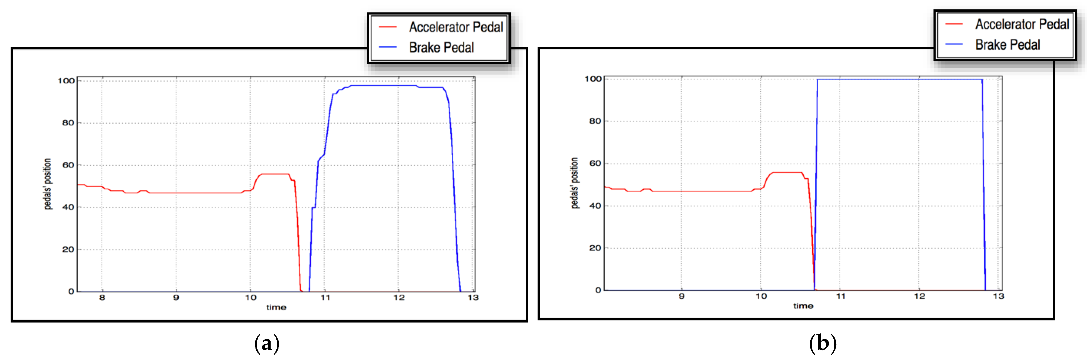
Due to the superiority of the evolved XGBoost classifier over the others, we integrated it into the braking assistant in the full-scale Forum-8 driving simulator. The sample dynamics of the accelerator and brake pedals in two cases of emergency braking—with and without automated braking activated by the driver-supporting agent—are shown in Figure 12.
6. Discussion
In a real-world driving situation, the most critical error might be in false positive cases, i.e., when automated braking is activated in an incorrectly classified emergency braking situation. It may seem that this error is a potentially dangerous one, as it may increase the likelihood of rear-end collision with the vehicle(s) traveling behind. However, our system is supposed to activate the emergency braking for a very brief period of time that is equivalent to the average delay of the driver’s response. We assume that the driver behind respects the common 3 s rule, which claims that each driver should always keep a safe distance in order to have enough time to respond to problems in front of his/her car.
As can be seen from Table 14, in the case of a wrongly classified situation the amount of braking would be insignificant, and would never cause a dangerous situation on the road. In cases of actual emergency braking situations, however, the driver would press the brake pedal just before the disengagement of the (brief) automated braking. This will ensure both early (due to the automated braking) and continuous (due to the driver’s input) braking of the car in actual emergency braking situations.
Nevertheless, our best classifier made several mistakes: 5 FN, 7 FP. Obviously, FN will not cause inconvenience to the driver; however, FP may lead to uncomfortable driving. It is probable that the incorrect classification is a result of either wrong sample marking by the expert in the testing set or wrong sample marking in the training set which caused the XGBoost classifier to learn on noisy samples. Another possible reason for the mistakenly classified samples might be the prevalence of similar driving style samples in the training dataset. For instance, if one driver prefers a fast driving style, the way he or she releases the accelerator pedal will definitely differ from the quiet driving style. This can result in “uncertain” output of the XGBoost classifier. For example, several instances from the training and testing sets have the output value close to 0.5, which indicates that XGBoost “doubts”. A way of improving this possible drawback will be investigated in further research.
7. Conclusions
We examined the feasibility of classifying the emergency braking situations in road vehicles solely from the motion pattern of the accelerator pedal. We compared the classifiers and employed genetic algorithms to tune the hyperparameters associated with them. With regard to the performance of all classifiers under consideration, XGBoost showed the best results for the EBC problem. The experimental results suggest that the evolved classifier detects the emergency braking situations with an accuracy of about 95% on the test set of offline time series data of the dynamics of the accelerator pedal.
In our future work, we are planning to investigate ways to further improve the quality of the classifier. We are considering alternative approaches for the training of the latter. Also, we intend to increase the data set and to get rid of noise (both for training and testing) in order to obtain more general and more robust classifier(s).
Our ultimate objective would be an implementation of a brake assistant that would be the best fit to the driving style of a particular driver. Thus, we contemplate an incremental approach of training the classifier: first, to train a general classifier offline on a wide set of training data and, then, to adapt the general classifier online to the driving style of a particular driver.
Acknowledgments
We would like to thank all testers for their volunteering and participating in the driving experiments. This research was funded in part by MEXT-supported Program for Strategic Research Foundation at Private Universities in Japan (2014–2018).
Author Contributions
Albert Podusenko and Ivan Tanev collected the data; Albert Podusenko and Vsevolod Nikulin processed the data; Albert Podusenko, Ivan Tanev and Katsunori Shimohara analyzed the data; Ivan Tanev programmed the genetic algorithms; Albert Podusenko implemented the learning of classifiers; Albert Podusenko wrote the paper.
Conflicts of Interest
The founding sponsors had no role in the design of the study; in the collection, analyses, or interpretation of data; in the writing of the manuscript, and in the decision to publish the results.
References
- Laukkonen, J. 13 Advanced Driver Assistance Systems. Available online: https://www.lifewire.com/advanced-driver-assistance-systems-534859 (accessed on 8 November 2017).
- Coelingh, E.; Eidehall, A.; Bengtsson, M. Collision Warning with Full Auto Brake and Pedestrian Detection—A Practical Example of Automatic Emergency Braking. In Proceedings of the 13th International IEEE Conference on Intelligent Transportation Systems, Funchal, Portugal, 19–22 September 2010; pp. 155–160. [Google Scholar] [CrossRef]
- Coelingh, E.; Jakobsson, L.; Lind, H.; Lindman, M. Collision Warning with Auto Brake—A Real-Life Safety Perspective. In Proceedings of the 20th International Technical Conference on the Enhanced Safety of Vehicles (ESV), Lyon, France, 18–21 June 2007. [Google Scholar]
- Kusano, K.D.; Gabler, H.C. Safety Benefits of Forward Collision Warning, Brake Assist, and Autonomous Braking Systems in Rear-End Collisions. IEEE Trans. Intell. Transp. Syst. 2012, 13, 1546–1555. [Google Scholar] [CrossRef]
- Fancher, P.; Bareket, Z.; Ervin, R. Human-Centered Design of an Acc-With Braking and Forward-Crash-Warning System. Int. J. Veh. Mech. Mobil. 2010, 36, 203–223. [Google Scholar]
- Wilde, G.J.S. The theory of risk homeostasis: Implications for safety and health. Risk Anal. 1982, 2, 209–225. [Google Scholar] [CrossRef]
- Haufe, S.; Treder, M.S.; Gugler, M.F.; Sagebaum, M.; Curio, G.; Blankertz, B. EEG potentials predict upcoming emergency brakings during simulated driving. J. Neural Eng. 2011, 8, 1–11. [Google Scholar] [CrossRef] [PubMed]
- Haufe, S.; Kim, J.; Kim, I.H.; Treder, M.S.; Sonnleitner, A.; Schrauf, M.; Curio, G.; Blankertz, B. Electrophysiology-based detection of emergency braking intention in real-world driving. J. Neural Eng. 2014, 11, 056011. [Google Scholar] [CrossRef] [PubMed]
- Kim, I.H.; Kim, J.W.; Haufe, S.; Lee, S.W. Detection of braking intention in diverse situations during simulated driving based on EEG feature combination. J. Neural Eng. 2015, 12, 016001. [Google Scholar] [CrossRef] [PubMed]
- Mccall, J.C.; Trivedi, M.M. Human Behavior Based Predictive Brake Assistance. In Proceedings of the 2006 IEEE Intelligent Vehicles Symposium, Tokyo, Japan, 13–15 June 2006; pp. 8–12. [Google Scholar] [CrossRef]
- Kassaagi, M.; Brissart, G.; Popieul, J.-C. A study on driver behavior during braking on open road. In Proceedings of the 18th International Technical Conference on the Enhanced Safety of Vehicles (ESV), Nagoya, Japan, 19–22 May 2003. [Google Scholar]
- Kiesewetter, W.; Klinkner, W.; Reichelt, W.; Steiner, M. Der neue Brake-Assist von Mercedes-Benz. Automobiltech. Z. 1997, 99, 330. [Google Scholar]
- Malta, L.; Miyajima, C.; Takeda, K. A Study of Driver Behavior under Potential Threats in Vehicle Traffic. IEEE Trans. Intell. Transp. Syst. 2009, 10, 201–210. [Google Scholar] [CrossRef]
- Podusenko, A.; Nikulin, V.; Tanev, I.; Shimohara, K. Cause and Effect Relationship between the Dynamics of Accelerator and Brake Pedals during Emergency Braking. In Proceedings of the FAST-zero 2017, Nara, Japan, 22–28 September 2017. [Google Scholar]
- Forum-8 Drive Simulator. Available online: http://www.forum8.co.jp/english/uc-win/road-drive-e.htm (accessed on 18 November 2017).
- Podusenko, A.; Nikulin, V.; Tanev, I.; Shimohara, K. Prediction of Emergency Braking Based on the Pattern of Lifting Motion of Accelerator Pedal; SICE: Osaka, Japan, 2017. [Google Scholar]
- Powers, D.M.W. Evaluation: From Precision, Recall and F-Measure to ROC. Inf. Mark. Correl. J. Mach. Learn. Technol. 2011, 2, 37–63. [Google Scholar]
- Kohavi, F. A Study of Cross-Validation and Bootstrap for Accuracy Estimation and Model Selection. In Proceedings of the 14th International Joint Conference on Artificial Intelligence, Montreal, QC, Canada, 20–25 August 1995. [Google Scholar]
- Refaeilzadeh, P.; Tang, L.; Liu, H. Cross-validation. In Encyclopedia of Database Systems; Springer: New York, NY, USA, 2009; pp. 532–538. [Google Scholar]
- Dasarathy, B.V. Nearest Neighbor (NN) Norms: NN Pattern Classification Techniques; IEEE Computer Society: Washington, DC, USA, 1991; ISBN 0-8186-8930-7. [Google Scholar]
- Suykens, J.; Vandewalle, J. Least Squares Support Vector Machine Classifiers. Neural Process. Lett. 1999, 9, 293. [Google Scholar] [CrossRef]
- Chen, T.; Guestrin, C. Xgboost: A Scalable Tree Boosting System. arXiv, 2016; arXiv:1603.02754. [Google Scholar]
- Adam-Bourdarios, C.; Cowan, G.; Germain-Renaud, C.; Guyon, I.; Kégl, B.; Rousseau, D. The Higgs Machine Learning Challenge. J. Phys. Conf. Ser. 2015. [Google Scholar] [CrossRef]
- Phoboo, A.E. Machine Learning wins the Higgs Challenge. ATLAS News, 20 November 2014. [Google Scholar]
- Lewis, R.J. An Introduction to Classification and Regression Tree (CART) Analysis. In Proceedings of the Annual Meeting of the Society for Academic Emergency Medicine, San Francisco, CA, USA, 22–25 May 2000. [Google Scholar]
- Goldberg, E.; Holland, J.H. Genetic Algorithms and Machine Learning. Mach. Learn. 1988, 3, 95–99. [Google Scholar] [CrossRef]
- Holland, J.H. Adaptation in Natural and Artificial Systems, Reprint edition; The MIT Press; Bradford Book: Cambridge, MA, USA, 1992. [Google Scholar]
- Holland, J.H. Hidden Order: How Adaptation Builds Complexity; Basic Books: New York, NY, USA, 1996. [Google Scholar]
- Pedregosa, F.; Varoquaux, G.; Gramfort, A.; Michel, V.; Thirion, B.; Grisel, O.; Blondel, M.; Prettenhofer, P.; Weiss, R.; Dubourg, V.; et al. Scikit-Learn: Machine Learning in Python. JMLR 2011, 12, 2825–2830. [Google Scholar]
- Buitinck, L.; Louppe, G.; Blondel, M.; Pedregosa, F.; Mueller, A.; Grisel, O.; Niculae, V.; Prettenhofer, P.; Gramfort, A.; Grobler, J.; et al. API Design for Machine Learning Software: Experiences from the Scikit-Learn Project. arXiv, 2013; arXiv:1309.0238. [Google Scholar]
- XGBoost Package. Available online: https://github.com/dmlc/xgboost (accessed on 18 November 2017).
- Podusenko, A. Classifiers Implementation of Emergency Braking Classifier in Python. 2017. Available online: http://isd-si.doshisha.ac.jp/a.podusenko/research (accessed on 18 November 2017).
Figure 1.
Typical dynamics of accelerator and brake pedals during (a) accelerating, (b) cruising, (c) slowing down (e.g., approaching corner), (d) normal braking (e.g., approaching a stop sign), and (e) emergency braking, respectively.
Figure 1.
Typical dynamics of accelerator and brake pedals during (a) accelerating, (b) cruising, (c) slowing down (e.g., approaching corner), (d) normal braking (e.g., approaching a stop sign), and (e) emergency braking, respectively.
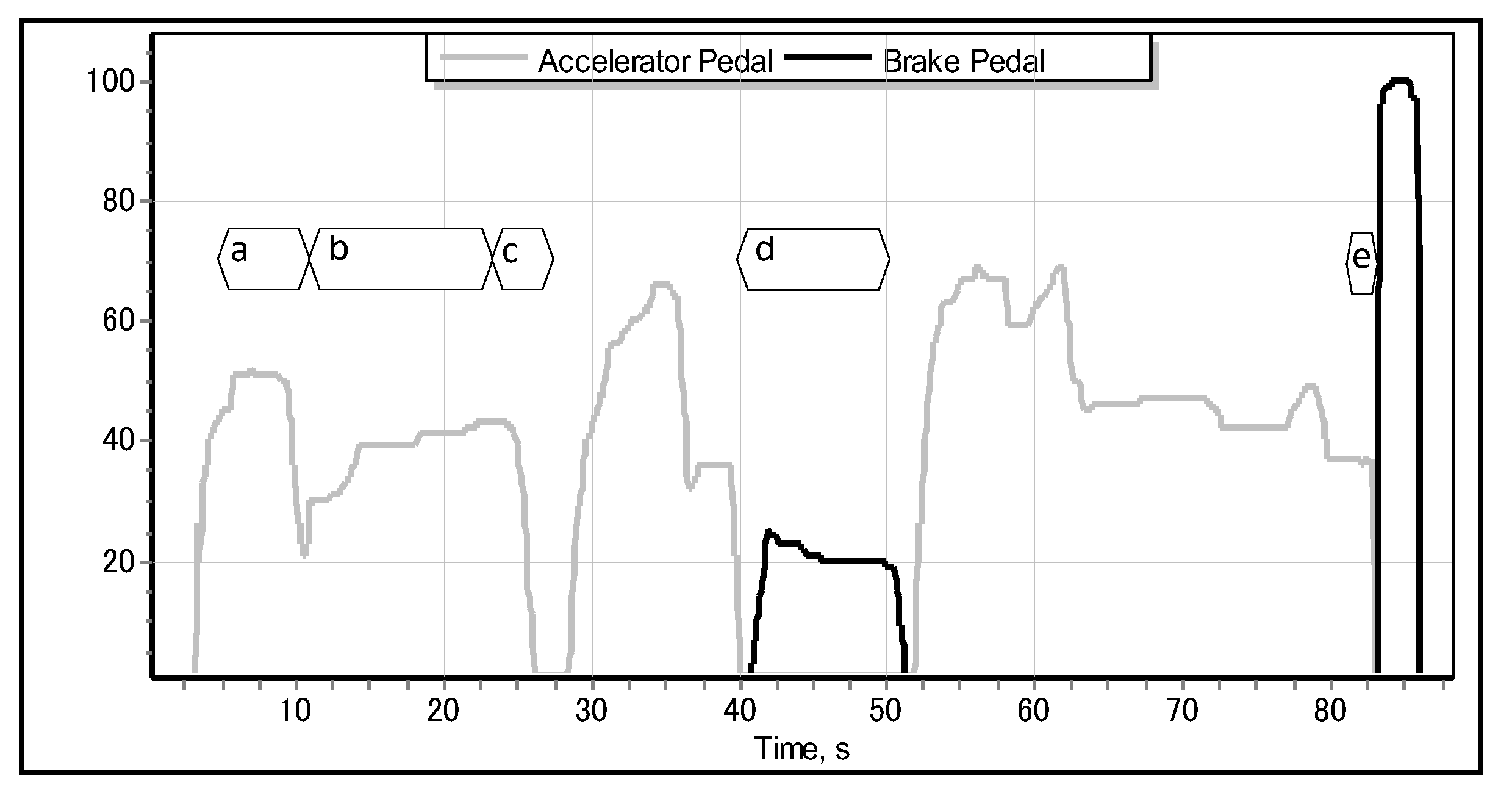
Figure 2.
Experimental environment: full-scale Forum-8 drive simulator.
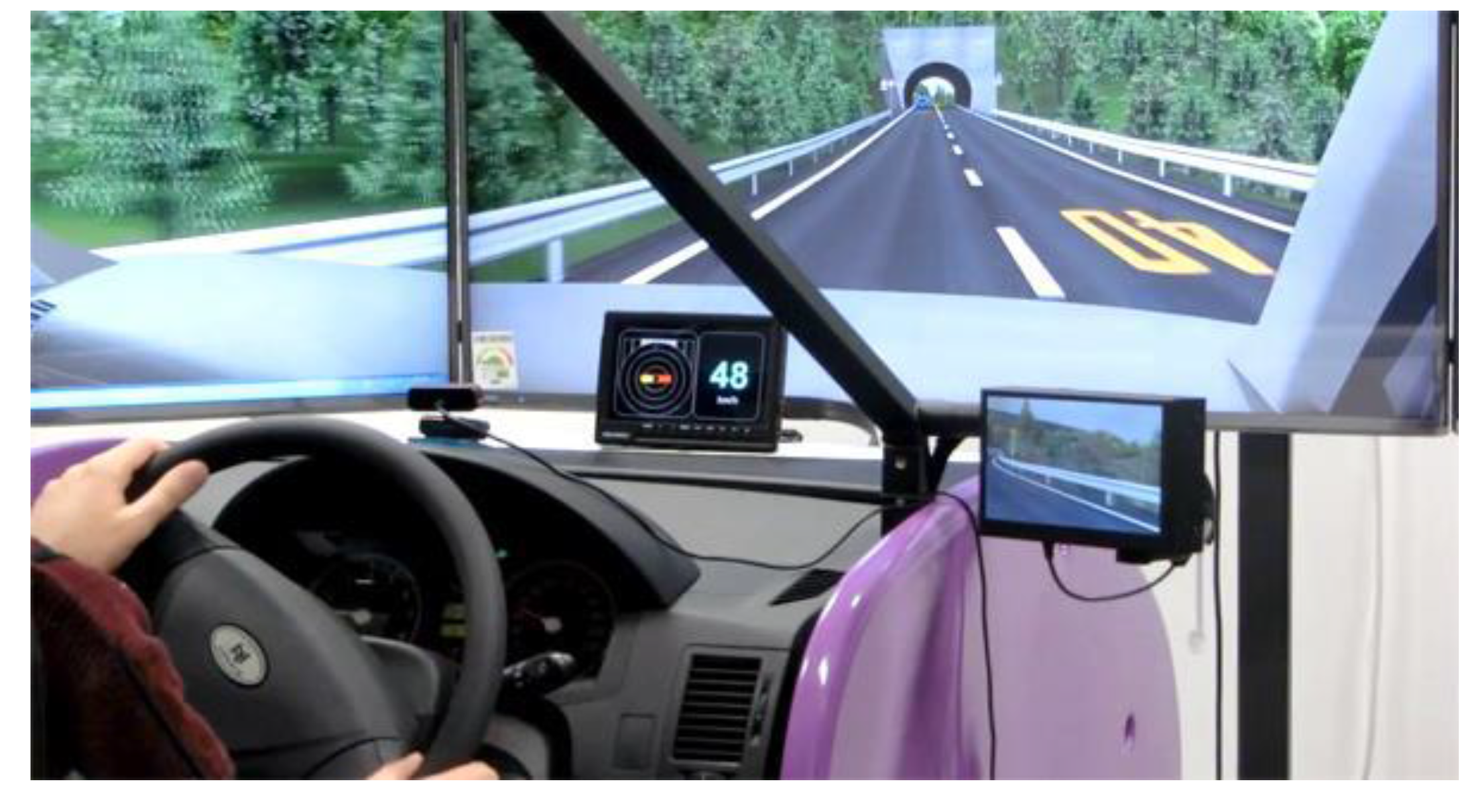
Figure 3.
Typical dynamics of accelerator and brake pedals during emergency braking. The braking behavior of the driver could be decomposed into the following three actions: lifting the accelerator (a), moving the right leg from accelerator to the brake pedal (b), and pressing the brake pedal to its (almost) maximum position (c). Depending on physical and cognitive condition of the driver, the corresponding time lags of these actions might significantly vary.
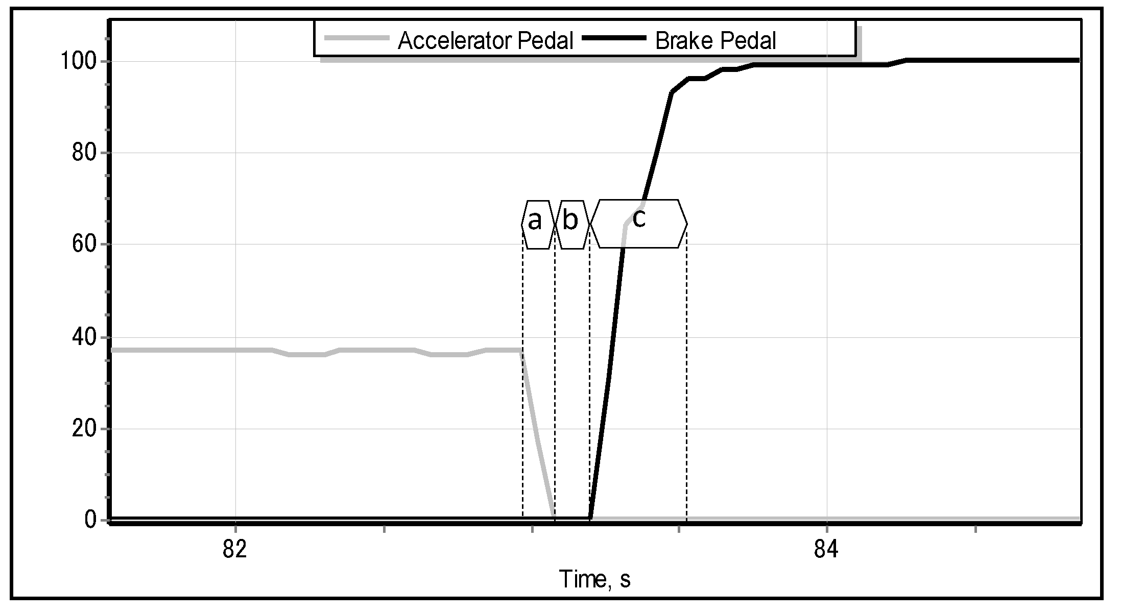
Figure 4.
K-fold cross-validation.
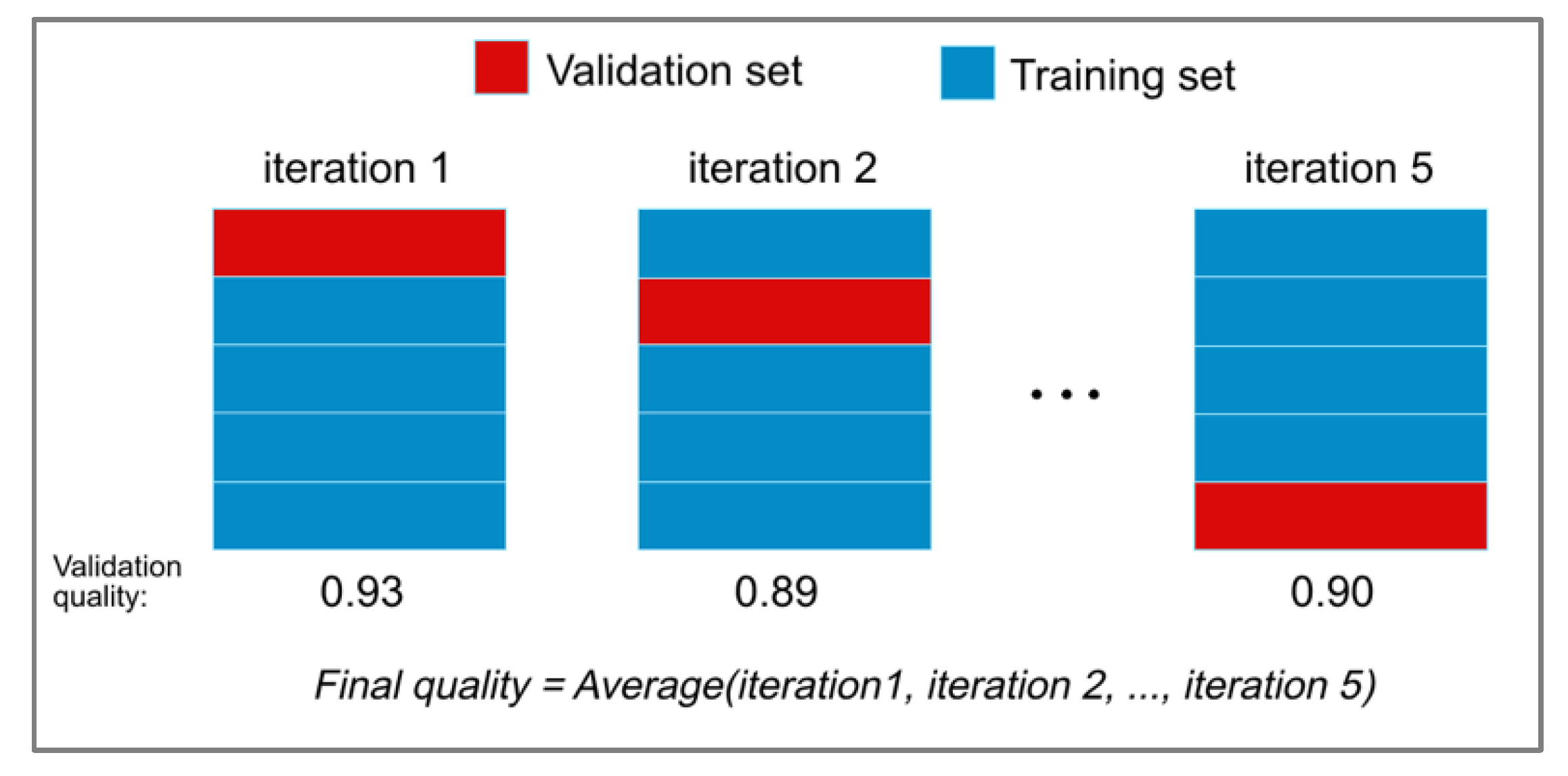
Figure 5.
Example of k-NN when k = 3.

Figure 6.
Examples of regularization parameter influence in the case of the two-dimensional classification problem. Red and blue points are training samples. The double arrow is hyperplane margin.
Figure 6.
Examples of regularization parameter influence in the case of the two-dimensional classification problem. Red and blue points are training samples. The double arrow is hyperplane margin.

Figure 7.
Breakdown of the time lag between lifting the accelerator and pressing the brake pedal completely, obtained from 383 events of emergency braking.
Figure 7.
Breakdown of the time lag between lifting the accelerator and pressing the brake pedal completely, obtained from 383 events of emergency braking.

Figure 8.
Relationship between the average rate of lifting the accelerator and the position of the pressed brake pedal.
Figure 8.
Relationship between the average rate of lifting the accelerator and the position of the pressed brake pedal.
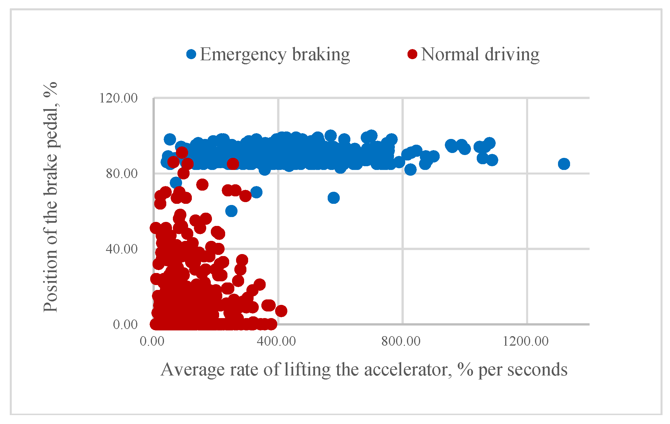
Figure 9.
Relationship between the maximum rate of lifting the accelerator and maximum rate of pressing the brake pedal.
Figure 9.
Relationship between the maximum rate of lifting the accelerator and maximum rate of pressing the brake pedal.
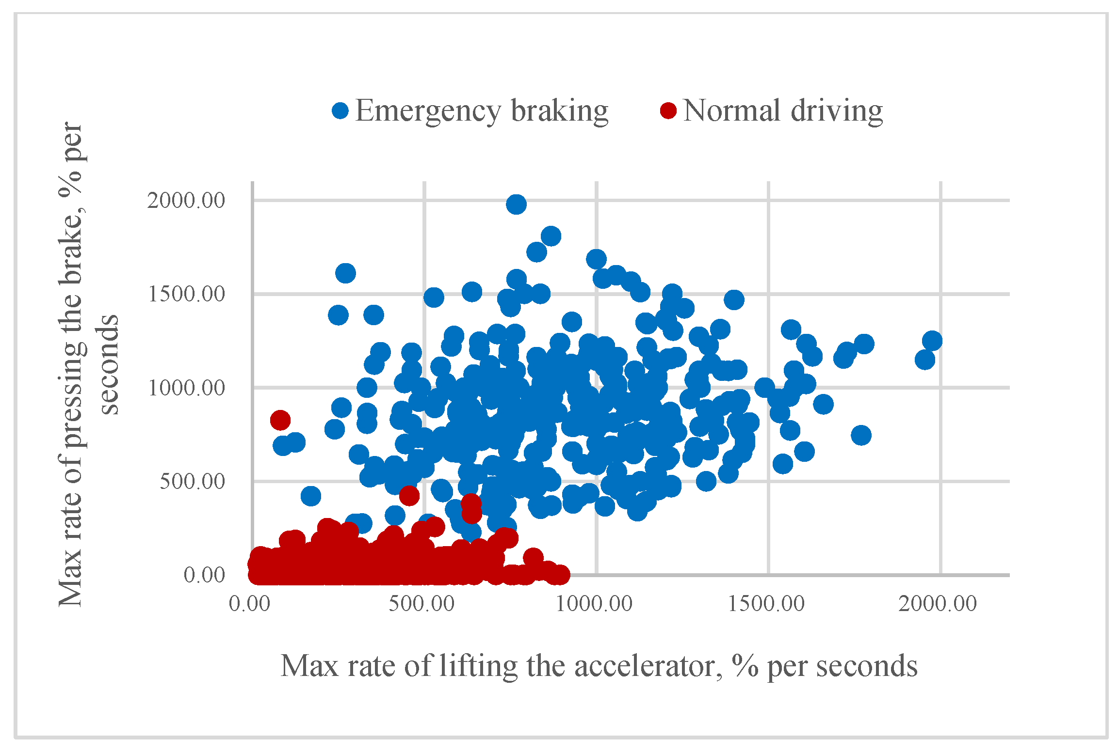
Figure 10.
Building process of the threshold classifier for aR feature.

Figure 11.
Fitness convergence characteristics obtained from 100 independent runs of GA employed for evolution of optimal hyperparameters of SVM (a) and XGBoost (b), respectively. The red line indicated the average (over 100 runs) of the fitness value.
Figure 11.
Fitness convergence characteristics obtained from 100 independent runs of GA employed for evolution of optimal hyperparameters of SVM (a) and XGBoost (b), respectively. The red line indicated the average (over 100 runs) of the fitness value.
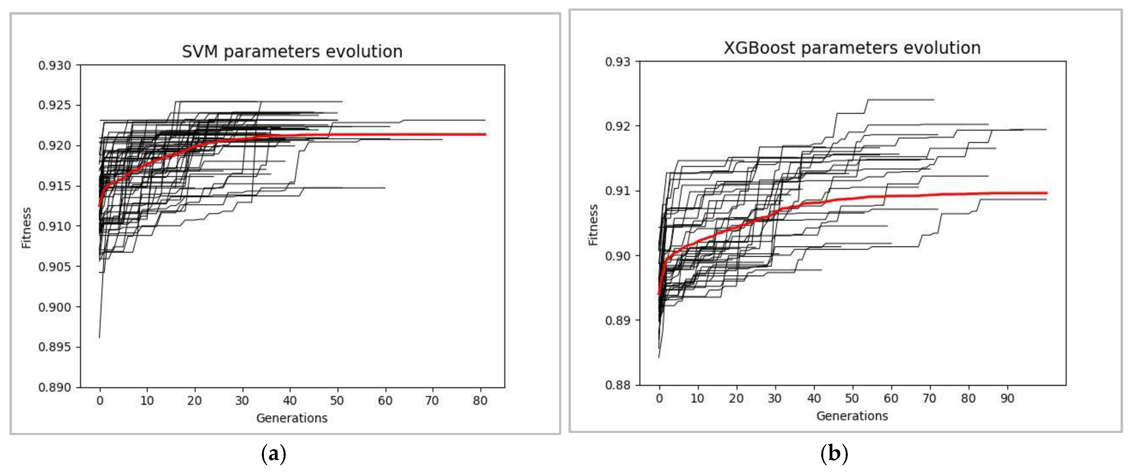
Figure 12.
Sample dynamics of accelerator and brake pedals in two cases of emergency braking: without (a) and with (b) automated braking activated by the driver-supporting agent.
Figure 12.
Sample dynamics of accelerator and brake pedals in two cases of emergency braking: without (a) and with (b) automated braking activated by the driver-supporting agent.

Table 1.
Confusion matrix.
| True Condition | |||
|---|---|---|---|
| Positive | Negative | ||
| Predicted condition | Positive | TP | FP |
| Negative | FN | TN | |
Table 2.
Details of the tracks used in experiments on Forum 8 full-scale drive simulator.
| Track | Length | Road Conditions | Traffic Conditions |
|---|---|---|---|
| Highway | 1 km | Dry | Moderate (high-speed) traffic |
| Countryside road | 3 km | Both dry and wet | Empty road (no traffic) |
| City road | 5 km | Both dry and wet | Dense (low-speed) traffic |
Table 3.
Details of the two series of experiments.
| Experiment | Range of the Position of Accelerator Pedal | Sampling Frequency, Hz | Requirements | Number of Data Samples |
|---|---|---|---|---|
| Normal driving | [0 … 100] | 25 | Emergency braking is not allowed | 529 |
| Emergency braking | [0 … 100] | 25 | Audible signal prompts the drivers to apply emergency braking | 775 |
Table 4.
Content of chromosome of GA applied for optimizing the values of hyperparameters of SVM.
| Allele (Hyperparameter) | Interval of Discretization | Range | Meaning |
|---|---|---|---|
| C | 0.002 | [0, 100] | Penalty parameter C of the error term |
| kernel | – | {linear, poly, rbf, sigmoid} | Specifies the kernel type to be used in SVM |
| degree | 1 | [1, 5] | Degree of the polynomial kernel function. Ignored by all other kernels |
| gamma | 0.1 | [0.01, 100] | Kernel coefficient for rbf, poly, and sigmoid |
| coef0 | 0.1 | [0.01, 100] | Independent term in kernel function. Significant in poly and sigmoid |
| shrinking | – | {True, False} | Whether to use shrinking heuristic |
Table 5.
Content of chromosome of GA applied for optimizing the values of hyperparameters of XGBoost.
Table 5.
Content of chromosome of GA applied for optimizing the values of hyperparameters of XGBoost.
| Allele (Hyperparameter) | Interval of Discretization | Range | Meaning |
|---|---|---|---|
| eta | 0.002 | [0, 1] | Step size shrinkage. Controls the learning rate in update and prevents overfitting |
| gamma | 0.1 | [0, 100] | Minimum loss reduction required to make a node split. Split happens when the resulting split gives a positive reduction in the loss function. |
| max_depth | 1 | [1, 20] | The maximum depth of a tree |
| min_child_weight | 1 | [1, 100] | Minimum sum of weights of all observations required in a child |
| subsample | 0.002 | (0.001, 1) | Subsample ratio of the training instance |
| colsample_bytree | 0.001 | (0.5, 1) | Subsample ratio of columns when constructing each tree |
| n_estimators | 1 | [100, 500] | The number of boosting stages to perform |
Table 6.
Main parameters of GA.
| Parameter | Value |
|---|---|
| Genotype | Each classifier has its own set of parameters (as shown in Table 4 and Table 5) encoded in the genotype. In addition, a fixed combination of features (pertinent to the dynamics of the accelerator pedal) is also incorporated into the genotype: {mP, aR}, {mP, mR}, {mR, aR}, {mP, aR, mR}, {mP, aR, mR, mP*aR}, {mP, aR, mR, mP*mR}, {mP, aR, mR, mR*aR} |
| Population size | 40 individuals |
| Selection | Binary Tournament |
| Selection ratio | 10% |
| Elite | Best 2 individuals |
| Crossover | Single-point |
| Mutation | Single-point |
| Mutation ratio | 5% |
| Fitness value | F-score |
| Termination criteria | (#Generations > 100) or (Fitness Value = 100%) |
Table 7.
Performance of simple threshold classifiers on training and testing set.
| Metric | Classifier Based on mR Feature | Classifier Based on aR Feature | ||
|---|---|---|---|---|
| Training Set | Testing Set | Training Set | Testing Set | |
| Accuracy | 0.769 | 0.791 | 0.888 | 0.873 |
| Precision | 1.000 | 1.000 | 0.964 | 0.980 |
| Recall | 0.461 | 0.513 | 0.671 | 0.610 |
| F-score | 0.631 | 0.677 | 0.791 | 0.752 |
Table 8.
Performance of k-NN classifier on training and testing set.
| Metric | 5-NN Method | 23-NN Method | ||
|---|---|---|---|---|
| Training Set | Testing Set | Training Set | Testing Set | |
| Accuracy | 0.944 | 0.938 | 0.926 | 0.95 |
| Precision | 0.937 | 0.867 | 0.918 | 0.896 |
| Recall | 0.933 | 0.951 | 0.908 | 0.951 |
| F-score | 0.935 | 0.907 | 0.913 | 0.923 |
Table 9.
Best-evolved values of hyperparameters of SVM.
| Allele (Hyperparameter) | Value Obtained via GA |
|---|---|
| C | 0.802 |
| kernel | rbf |
| gamma | 0.8 |
| coef0 | 9.0 |
| shrinkage | True |
| features | {mP, aR, mR} |
Table 10.
Best-evolved values of hyperparameters of XGBoost.
| Allele (Hyperparameter) | Optimal Value Obtained via GA |
|---|---|
| eta | 0.374 |
| gamma | 6.6 |
| max_depth | 3 |
| min_child_weight | 2 |
| subsample | 0.454546 |
| colsample_bytree | 0.624 |
| n_estimators | 96 |
| features | {mP, aR, mR, mP*aR} |
Table 11.
Performance of SVM classifiers on training and testing sets.
| Metric | Default SVM Classifier | Evolved SVM Classifier | ||
|---|---|---|---|---|
| Training Set | Testing Set | Training Set | Testing Set | |
| Accuracy | 0.9348 | 0.95 | 0.9396 | 0.95 |
| Precision | 0.9479 | 0.9058 | 0.9465 | 0.9058 |
| Recall | 0.8971 | 0.939 | 0.9105 | 0.939 |
| F-score | 0.9218 | 0.9221 | 0.9281 | 0.9221 |
Table 12.
Performance of evolved XGBoost classifier on training and testing sets.
| Metric | Default XGBoost | Evolved XGBoost | ||
|---|---|---|---|---|
| Training Set | Testing Set | Training Set | Testing Set | |
| Accuracy | 0.9502 | 0.9461 | 0.953 | 0.9538 |
| Precision | 0.954 | 0.8953 | 0.9461 | 0.917 |
| Recall | 0.9284 | 0.939 | 0.944 | 0.939 |
| F-score | 0.941 | 0.917 | 0.9451 | 0.9277 |
Table 13.
Comparison of best classifiers.
| Metric | 23-NN Method | Default (and Evolved) SVM | Evolved XGBoost |
|---|---|---|---|
| Accuracy | 0.95 | 0.95 | 0.9538 |
| Precision | 0.896 | 0.9058 | 0.917 |
| Recall | 0.951 | 0.939 | 0.939 |
| F-score | 0.923 | 0.9221 | 0.9277 |
Table 14.
The effect of FP on the reduction of distances to the following car.
| Speed of the Car | Distance between Two Cars, m | Reduction of the Distance to the Following Car as a Result of Eventual False Positive Emergency Braking of 200 ms, m | ||
|---|---|---|---|---|
| km/h | m/s | For 3 s Interval between Cars (Marginal) | For 6 s Interval between Cars (Good) | |
| 36 | 10 | 30 | 60 | 2 |
| 54 | 15 | 45 | 90 | 3 |
| 72 | 20 | 60 | 180 | 4 |
| 90 | 25 | 75 | 150 | 5 |
| 108 | 30 | 90 | 180 | 6 |
| 126 | 35 | 105 | 210 | 7 |
© 2017 by the authors. Licensee MDPI, Basel, Switzerland. This article is an open access article distributed under the terms and conditions of the Creative Commons Attribution (CC BY) license (http://creativecommons.org/licenses/by/4.0/).
Share and Cite
MDPI and ACS Style
Podusenko, A.; Nikulin, V.; Tanev, I.; Shimohara, K. Comparative Analysis of Classifiers for Classification of Emergency Braking of Road Motor Vehicles. Algorithms 2017, 10, 129. https://doi.org/10.3390/a10040129
AMA Style
Podusenko A, Nikulin V, Tanev I, Shimohara K. Comparative Analysis of Classifiers for Classification of Emergency Braking of Road Motor Vehicles. Algorithms. 2017; 10(4):129. https://doi.org/10.3390/a10040129
Chicago/Turabian StylePodusenko, Albert, Vsevolod Nikulin, Ivan Tanev, and Katsunori Shimohara. 2017. "Comparative Analysis of Classifiers for Classification of Emergency Braking of Road Motor Vehicles" Algorithms 10, no. 4: 129. https://doi.org/10.3390/a10040129
Note that from the first issue of 2016, this journal uses article numbers instead of page numbers. See further details here.