WSN Nodes Placement Optimization Based on a Weighted Centroid Artificial Fish Swarm Algorithm

Abstract

Aiming at optimal placement of wireless sensor network (WSN) nodes of wind turbine blade for health inspection, a weighted centroid artificial fish swarm algorithm (WC-AFSA) is proposed. A weighted centroid algorithm is applied to construct an initial fish population so to enhance the fish diversity and improve the search precision. Adaptive step based on dynamic parameter is used to jump out local optimal solution and improve the convergence speed. Optimal sensor placement is realized by minimizing the maximum off-diagonal elements of the modal assurance criterion as the objective function. Five typical test functions are applied to verify the effectiveness of the algorithm, and optimal placement of WSNs nodes on wind turbine blade is carried out. The results show that WC-AFSA has better optimization effect than AFSA, which can solve the problem of optimal arrangement of blade WSNs nodes.

1. Introduction

Blade is one of the key components of the wind turbine. It is responsible for converting wind energy into rotational mechanical energy of wind turbine rotors. The wind turbine blade is extremely easy to suffer varying degrees of damage under the influence of environment of wind, sand, ice, thunder and lightning, as well as a variety of stress concentrations, leading to the shutdown of the wind turbine, and serious economic losses. The volume and mass of wind turbine blade are huge, so it is difficult to maintain manually, with high maintenance costs. Therefore, in order to decrease the risk of operation, while reducing maintenance costs, it is of great significance to carry out health monitoring in the wind turbine blade structure, especially identify the damage state quickly and accurately [1,2].

In this work, modal test is made for the health monitoring of blades. Attach a certain number of sensors on the blades to extract modal parameters. Due to the relative motion between the blades and cabin, it is inconvenient to transmit data through wired mode. At the same time, owing to the large number of sensors and complex wire arrangement, it is very convenient to use wireless sensors to transmit the real-time information about blade’s health state to receiver.

Wireless sensor networks (WSNs) [3] are usually deployed in complex monitoring areas where the environment is harsh and is inaccessible to people. Deployment of WSNs can enlarge the transmission distance and make the system not easily disturbed by the environment. The wireless sensor network adopts an ad hoc network and multi-hop technology, which greatly reduces the cost of the monitoring system, and makes the installation and maintenance of the sensor network very convenient and fast. By changing the topology of the network in WSNs dynamically, energy consumption is reduced, network capacity and life are increased and collisions between nodes are avoided [4,5]. The topology control of WSNs is divided into the network topology establishment stage and the network topology maintenance stage. To ensure that the complex topology can operate, as well as the simple topology built initially, a reasonable topology control algorithm is needed [6]. WSNs technology has attracted more and more attention in recent years [7,8].

By means of WSNs, we can collect, process, and analyze the data reflecting the blade’s health state. However, there are few studies on the optimal placement of WSNs for wind turbine blades monitoring. The artificial fish swarm algorithm (AFSA) is a new kind of swarm intelligence optimization algorithm based on the behavior of fish [9,10]. The basic idea of AFSA is to imitate the fish behaviors such as prey, swarm, and follow. AFSA is simple in principle and has some good features such as robustness, and tolerance of parameter setting. This algorithm has some disadvantages yet. Non-uniform distribution deduced by randomly generating initial fish population decreases the global search ability of the algorithm. The search step of each fish is fixed. At the early iteration, the algorithm is easy to fall into local minimum.

To solve the above problems, a weighted centroid algorithm (WCA) [11] is introduced to the artificial fish swarm algorithm (AFSA) to initialize the fish swarm in this work. By measuring the distance between nodes, localization compensation error and adaptive search step, the convergence speed and optimization precision are improved.

2. Mathematical Model of Blades WSNs Nodes Optimal Placement

To carry out finite element model (FEM), the essential is to obtain the three mechanical properties: displacement, strain and stress. For the complex structure like wind turbine blades, after analyzing the above three mechanical properties, we can evaluate the structures’ strength and stiffness to obtain the structure’s vibration characteristics parameters such as frequency and mode shapes which provide theory support for structure health monitoring, damage identification and analysis of dynamic characteristics.

Establish the FEM of wind turbine blade, and extract mode shape matrix ${\mathit{\varphi }}_{\mathrm{n}\times \mathrm{m}}$. n denotes the number of degrees of freedom (DOFs), namely, the number of candidate sensor positions. m denotes the order number of mode shapes. Select s DOFs from n DOFs as the final sensor locations. In order to ensure the measured modal vectors being easily distinguished, modal assurance criterion (MAC) [12] is applied to evaluate the measured modal vectors. The maximum off-diagonal element of MAC is taken as the objective function of minimum problem. The mathematical model can be expressed as:

$$f({\mathit{\varphi }}_{\mathrm{s}\times \mathrm{m}})=\max \{\mathrm{M}\mathrm{A}{\mathrm{C}}_{ij}=\frac{{\left({\mathit{\varphi }}_i^{\mathrm{T}}{\mathit{\varphi }}_j\right)}^2}{\left({\mathit{\varphi }}_i^{\mathrm{T}}{\mathit{\varphi }}_i\right)\left({\mathit{\varphi }}_j^{\mathrm{T}}{\mathit{\varphi }}_j\right)}\}.$$

(1)

where $0\le f({\mathit{\varphi }}_{\mathrm{s}\times \mathrm{m}})\le 1$. ${\mathit{\varphi }}_i$ and ${\mathit{\varphi }}_j$ represent the ith and jth column vectors in matrix Φ, respectively. The superscript T denotes the transpose of the vector. If the off-diagonal elements of $\mathrm{M}\mathrm{A}{\mathrm{C}}_{\mathrm{i}\mathrm{j}}$($i\ne j$) tend to zero, which indicates that there is little correlation between the modal vector i and j, that is to say, the modal vector can be distinguished easily.

The objective function of blade WSNs nodes optimal placement can be expressed as:

$$\mathrm{m}\mathrm{i}\mathrm{n}f(x)=\underset{i\ne j}{\mathrm{m}\mathrm{a}\mathrm{x}}\left\{\mathrm{M}\mathrm{A}{C}_i{}_j\right\}.$$

(2)

3. Weighted Centroid Fish Swarm Algorithm

In this paper, the weighted centroid fish swarm algorithm is used for global search. The weighted centroid algorithm and adaptive search step are introduced to improve the search capability.

3.1. Procedure of the Weighted Centroid Fish Swarm Algorithm

3.1.1. Principle of the AFSA

In water, fish are most likely distributed around the field with the most abundant food. A fish swarm completes its food foraging process by several social behaviors. AFSA, inspired by the behaviors of fish, is a novel method for searching the global optimum. It is a random search algorithm based on simulating fish swarm behaviors, which include prey behavior, swarm behavior, follow behavior and random behavior.

Suppose the current state of an artificial fish is $X=(x_1,x_2,\dots ,x_n)$. Visual is the perception scope of an artificial fish, which determines the moving direction of each artificial fish. Step is the maximum moving step length. To avoid missing the optimal solutions, Step should not be set too large.$X_v=(x_1,x_2,\dots ,x_n)$ is the location at certain moment. Visual and Step are shown in Figure 1.

$$X_{next}=X+rand()\times Step\times \frac{X_v-X}{\left|X_v-X\right|}$$

(3)

where rand ( ) produces random number between 0 and 1.

3.1.2. Binary Coding

Binary coding is intuitive and convenient for the optimal sensor placement problem [13]. Let n denote the initial number of candidate sensors and s denote the final number of sensors determined. The binary coding for a solution can be expressed as $\mathit{X}={(x_0,x_1,\dots ,x_j,\dots ,x_n)}^{\mathrm{T}}$, $j\in \left\{1,2,\dots ,n\right\}$. If $x_j=1$, there is a sensor on that DOF. If $x_j=0$, there is no sensor on that DOF. The condition ${\displaystyle \sum _{j=1}^n{x}_j}=s$ is satisfied.

The conversion between binary coding X and modal matrix ${\mathit{\varphi }}_{\mathrm{s}\times \mathrm{m}}$ is the process of removing the rows of ${\mathit{\varphi }}_{n\times \mathrm{m}}$. In this process, remove those rows of ${\mathit{\varphi }}_{n\times \mathrm{m}}$ corresponding to those $\{x_j|x_j=0,j\in [1,2,\dots ,n]\}$ in X. For convenience, this process is represented by Equation (4):

$${\mathit{\varphi }}_{s\times m}=\mathit{g}({\mathit{\varphi }}_{n\times m},{\mathit{X}}_{n\times 1})$$

(4)

where the modal matrix ${\mathit{\varphi }}_{s\times m}$ is a solution for placing s sensors in optimal sensor placement; ${\mathit{X}}_{n\times 1}$ is the binary coding corresponding to a solution.

For a simple example, substituting $n=4$, $m=2$, $s=3$ and ${\mathit{X}}_{4\times 1}={(1,0,1,1)}^{\mathrm{T}}$ into Equation (4), and take ${\mathit{\Phi }}_{4\times 2}=\left[\begin{array}{c}1\\ 2\\ 3\\ 4\end{array}\begin{array}{c}5\\ 6\\ 7\\ 8\end{array}\right]$ as the input modal matrix of function g, the output modal matrix of g is ${\mathit{\Phi }}_{3\times 2}=\mathit{g}\left(\left[\begin{array}{c}1\\ 2\\ 3\\ 4\end{array}\begin{array}{c}5\\ 6\\ 7\\ 8\end{array}\right],\left[\begin{array}{c}1\\ 0\\ 1\\ 1\end{array}\right]\right)=\left[\begin{array}{c}1\\ \xcancel{2}\\ 3\\ 4\end{array}\begin{array}{c}5\\ \xcancel{6}\\ 7\\ 8\end{array}\right]=\left[\begin{array}{cc}1& 5\\ 3& 7\\ 4& 8\end{array}\right]$ and can be easily obtained by deleting the second row of ${\mathit{\Phi }}_{4\times 2}$.

3.1.3. Fish Swarm Initialization through WCA

The core of the centroid algorithm (CA) is that unknown nodes estimate its location according to the geometric center combined with all its communications anchor nodes [11]. The principle of centroid algorithm is shown in Figure 2.

In Figure 2, solid dots $\mathrm{A}(x_1,y_1)$, $\mathrm{B}(x_2,y_2)$ and $\mathrm{C}(x_3,y_3)$ are the anchor nodes, and hollow dot $\mathrm{D}(X,Y)$is the unknown nodes to be located. a, b, c are the distances between D and A, B, and C respectively.

Select three nodes close to D to form trigon. Determine the trigon centroid. This is the location to be determined, which is expressed as:

$$(\overline{X},\overline{Y})=(\frac{1}{n}{\displaystyle \sum _{i=1}^n{\overline{x}}_i},\frac{1}{n}{\displaystyle \sum _{i=1}^n{\overline{y}}_i})$$

(5)

where n is the number of anchor nodes.

The location $(\overline{X},\overline{Y})$ of the nodes to be located is estimated based on the distance centroid method. Let T the uniform distributed random number between 0 and 1. Generate the initial fish swarm:

$$\{\begin{array}{l}x=\overline{X}+{(-1)}^{[T\times 10]}\times T\times {\delta }_x\\ y=\overline{Y}+{(-1)}^{[T\times 10]}\times T\times {\delta }_y\end{array}$$

(6)

where ${\delta }_x=\left|\overline{X}\right|/2$, ${\delta }_y=\left|\overline{Y}\right|/2$.

The weighed centroid algorithm (WCA) rationally distributes the weights to make the location more precise. The less distance between the unknown node and anchor node, the greater the impact of the anchor node on the unknown node [14]. WCA can be expressed as:

$$P_i(x,y)={\displaystyle \sum _{}^N(w_{ij}\times B_j(x,y))/}{\displaystyle \sum _{}^N{w}_{ij}}$$

(7)

where $w_{ij}$ is the weight of anchor node j to unknown node i, and $w_{ij}=1/{(d_{ij})}^n$; $P_i(x,y)$ is the estimated location of unknown node i; $B_j(x,y)$ is the location of the anchor node j; $d_{ij}$ is the distance between the anchor node j and the unknown node i; n is weight coefficient ranging from 1 to 4; N is the number of the anchor nodes.

The average error location can be expressed as:

$$ERROR=\frac{1}{N\times R}{\displaystyle \sum _{i=1}^N\sqrt{{\left(x_i-{\overline{x}}_i\right)}^2+{\left(y_i-{\overline{y}}_i\right)}^2}}$$

(8)

where $(x_i,y_i)$ is the actual location of the unknown node; $({\overline{x}}_i,{\overline{y}}_i)$ is the estimate location of the unknown node; R is the radio range of WSNs.

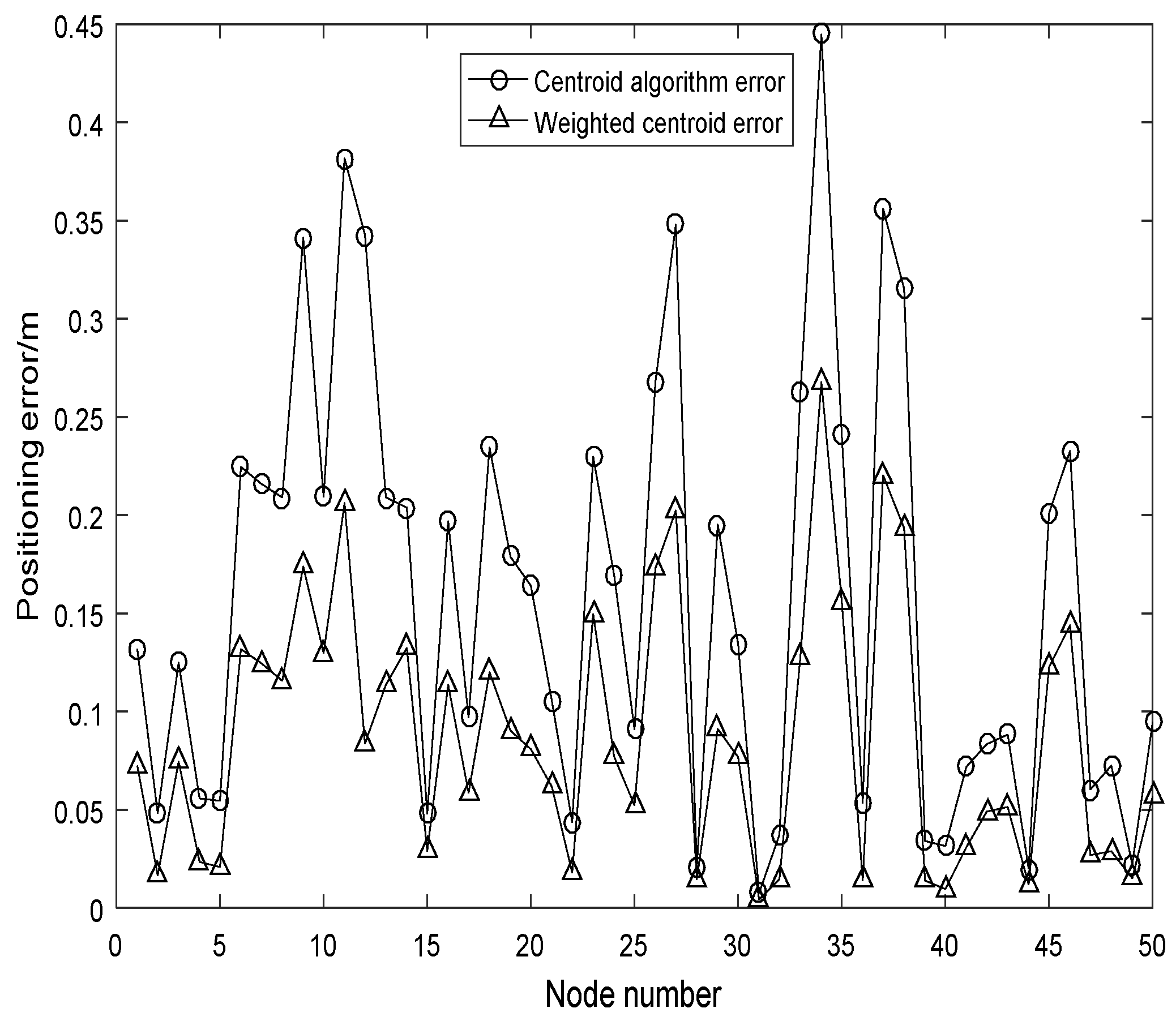
Figure 3 shows 50 WSNs nodes uniformly distributed with $100\times 100$ m area. Suppose R is 50 m. From Figure 4, the error of CA is larger than that of WCA. The location determined by WCA is closer to actual location and more accurate.

3.1.4. Swarm Behavior

An artificial fish tends to move toward the central location of fish swarm. This is the swarm behavior. Swarm behavior is the main process for search local optimization, and the search time is longer. step and the maximum iterations $N_{\max }$ affect the accuracy and convergence speed of the algorithm. The larger step and the smaller $N_{\mathrm{m}\mathrm{a}\mathrm{x}}$, the faster convergence speed but lower precision. So, proper step should be determined. Here, we adopt one kind of adaptive step. In the early iteration, large step is used to accelerate convergence speed. With the increase of the number of iterations, the optimum solution is gradually approximated, then adopt a small step to refine the search and improve search precision.

Assuming that the current iteration number is $N<N_{\mathrm{m}\mathrm{a}\mathrm{x}}$, the current state of an artificial fish is ${\mathit{x}}_i$. Its fitness function is $f({\mathit{x}}_i)$. A new state within visual is ${\mathit{x}}_j$, and the fitness function is $f({\mathit{x}}_j)$. If $f({\mathit{x}}_j)<f({\mathit{x}}_i)$, then we choose the moving $Step=rand()\times \Vert x_j-x_i\Vert$. Adding the function rand ( ) is to get into the local optimum in order to prevent its convergence too quickly.

3.1.5. Follow Behavior

When one or several fish find a field where there is more food and it is not crowded, the fish nearby will follow and move toward the food. This is the follow behavior. For the i-fish, the procedure of follow behavior is as follows:

Step 1: Randomly generate new location of artificial fish within ${\mathit{x}}_i{}^{\prime }$ on the interval $[x_{ij}-visual,x_{ij}+visual]$, $j=1,2,\dots ,n$;

Step 2: Compute food concentration$f({\mathit{x}}_i{}^{’})$. If $\frac{f({\mathit{x}}_i{}^{’})}{n_f}>\delta f({\mathit{x}}_i)$, the new fish moves toward a new location;

Step 3: Repeat (1), (2) until $N_{\max }$ is reached.

3.1.6. Prey Behavior

An artificial fish follows the direction with high food concentration in prey behavior. Suppose the current state of an artificial fish is ${\mathit{x}}_i$. Randomly select a new state $x_j$ within visual. If the food concentration is $f({\mathit{x}}_j)<f({\mathit{x}}_i)$, the artificial fish moves one step toward ${\mathit{x}}_j$; otherwise, randomly reselect ${\mathit{x}}_j$and judge whether it satisfies the condition of moving forward. If the condition cannot be satisfied until try_number is reached, the artificial fish randomly moves one step within visual.

3.2. Advantage Analysis of the Adaptive Step

The AFSA has a strong global search ability. However, in later iterations, the fish swarm gathers near the peak value, which makes the bot search precision and convergence speed slow. If the fixed step is large, it is easy to jump out of the optimal solution, but the accuracy of calculation is low. If the fixed step is small, the precision is improved, but the convergence speed is slow, it is easy to fall into the local optimum and difficult to jump out.

To solve the above problems, an adaptive step is introduced. In the initial optimization, the artificial fish, which is far away from the optimal value, adopts larger step to approach the optimum value quickly. When approaching the optimal value, make use of smaller step to improve the accuracy. The introduction of the adaptive step not only accelerates the convergence speed but also improves the accuracy of the solution.

3.3. Time Complexity Analysis

The effectiveness of the algorithm can be measured by time complexity. The basic operation count is regarded as the time complexity of the algorithm. We analyze the time complexity according to the implementation procedure of WCA-AFSA.

• Initialization of N artificial fish needs N times. Time complexity is $O(N)$.
• Initialization of other parameters assigns once and compares $N-1$ times. Time complexity is $O(N)$.
• Swarm behavior computes crowding factor N times, judges once, moves once, and swarms N times. Time complexity is $O(N^2+2\times N)$.
• Follow behavior searches the optimal value N times, computes crowding factor N times, judges once, moves once, and follows N times. Time complexity is $O(2\times N^2+2\times N)$.
• The frequency of prey behavior is, at most, try_number times, at least once. N artificial fishes prey N times. Time complexity is $O(N\times \mathit{\text{try\_number}})$.

After l iterations, time complexity is $O(l\times (3\times N^2+N\times \mathit{\text{try\_number}}+4\times N))$.

3.4. Procedure of WCA-AFSA

Step 1: Initialize fish swarm. N is the size of artificial fish swarm. Set the number of maximum iterations, try the number of prey behavior, perception scope, initial step, and factor of crowding degree as $N_{\max }$, try_number, visual, a, and $\delta$ respectively.

Step 2: Obtain the maximum off-diagonal element of MAC. On the basis of modal matrix ${\mathit{\varphi }}_{n\times m}$, compute the objective function of each artificial fish according to Equation (2).

Step 3: Execute swarm and prey behavior. Move toward the direction of small objective function. If two behaviors both cannot satisfy the condition of moving forward, perform prey behavior. If try_number is reached and still cannot satisfy the condition of moving forward, carry out a random behavior.

Step 4: Re-compute the objective function value of each fish. If $N_{\max }$ is reached then execute (5); otherwise execute (3).

Step 5: Determine the optimal solution according to Equation (2).

The flow chart of WCA-AFSA is depicted in Figure 5.

4. WCA-AFSA Performance Test

Five benchmark functions, which include the Sphere function, Ackley function, Rastrigin function, Griewank function, and Rosenbrock function, are applied to verify the performance of the WCA-AFSA. These functions all have the features of multiple peaks and high dimension.

(1)

Sphere function:

$$f_1(x)={\displaystyle \sum _{i=1}^n{x}_i^2},x_{\mathrm{i}}\in [-100,100],f_{\mathrm{m}\mathrm{i}\mathrm{n}}=0$$

(2)

Ackley’s function:

$$f_2(x)=-20\exp (-0.2\sqrt{\frac{1}{n}{\displaystyle \sum _{\mathrm{i}=1}^n{x}_i{}^2}})-\mathrm{e}\mathrm{x}\mathrm{p}(\frac{1}{n}{\displaystyle \sum _{\mathrm{i}=1}^n\mathrm{c}\mathrm{o}\mathrm{s}(2\pi x_i}))+20+\mathrm{e}\mathrm{x}\mathrm{p}(1),x_i\in [-32.768,32.768],f_{\mathrm{m}\mathrm{i}\mathrm{n}}=0$$

(3)

Generalized Rastrigin’s function:

$$f_3(x)={\displaystyle \sum _{i=1}^n(x_i^2}-10\mathrm{c}\mathrm{o}\mathrm{s}(2\pi x_i)+10),x_i\in [-5.12,5.12],f_{\mathrm{m}\mathrm{i}\mathrm{n}}=0$$

(4)

Generalized Griewank’s function:

$$f_4(x)={\displaystyle \sum _{i=1}^n\frac{x_i^2}{4000}}-{\displaystyle \prod _{i=1}^n\mathrm{c}\mathrm{o}\mathrm{s}(\frac{x_i}{\sqrt{i}}})+1,x_i\in [-600,600],f_{\mathrm{m}\mathrm{i}\mathrm{n}}=0$$

(5)

Generalized Rosenbrock’s function:

$$f_5(x)={\displaystyle \sum _{i=1}^n[100(x_{i+1}-x_i^2}{)}^2+{(1-x_i)}^2]$$

$f_1(x)$ and $f_2(x)$ used for testing convergence speed and precision are single modal functions with single extreme values. $f_3(x)$ and $f_4(x)$ used for testing the global search ability are multiple modal functions with nonlinear multiple extreme values. $f_5(x)$ is an abnormal function, which is applied for testing the algorithm performance.

Set the size of the artificial fish swarm N = 20, initial step = 0.5, and the number of maximum iterations $N_{\mathrm{m}\mathrm{a}\mathrm{x}}$ = 120. The average value is listed in

Table 1. Test results.

Function	Optimal Theoretical Value	Optimal Actual Average Value		Average Time/s
		${\mathit{f}}_{\mathit{W}\mathit{C}\mathit{A}-\mathit{A}\mathit{F}\mathit{S}\mathit{A}}$	${\mathit{f}}_{\mathit{A}\mathit{F}\mathit{S}\mathit{A}}$	${\mathit{T}}_{\mathit{W}\mathit{C}\mathit{A}-\mathit{A}\mathit{F}\mathit{S}\mathit{A}}$	${\mathit{T}}_{\mathit{A}\mathit{F}\mathit{S}\mathit{A}}$
$f_1(x)$	0	0.0035	0.0099	49.203655	50.245561
$f_2(x)$	0	0.0012	0.0040	48.945043	50.062352
$f_3(x)$	0	0.0427	0.1498	49.671079	50.784103
$f_4(x)$	0	$4.0878\times {10}^{-5}$	$5.9343\times 1{10}^{-5}$	49.660634	49.887099
$f_5(x)$	0	0.0052	0.0123	49.686631	50.670954

.

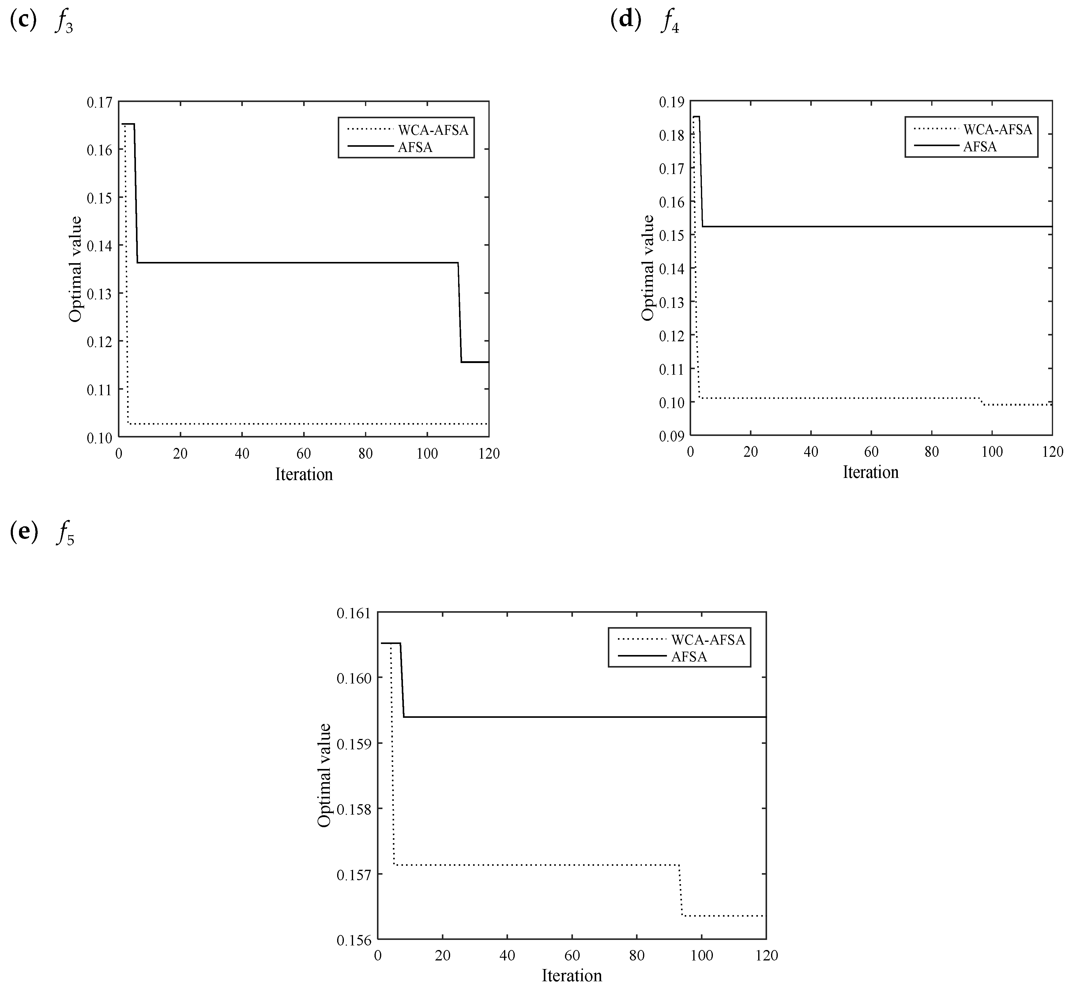
From Table 1, the optimal actual average value by WCA-AFSA is smaller than that by AFSA. It demonstrates WCA-AFSA has higher convergence accuracy. The average time of WCA-AFSA is shorter than that by AFSA. It indicates WCA-AFSA is more effective. Figure 6 shows the comparison of the results.

WCA-AFSA has better convergence precision and speed than AFSA. This means WCA-AFSA has better search ability.

5. WSNs Nodes Optimal Placement Based on WCA-AFSA

5.1. Example of a Wind Turbine Blade

For a one megawatt level horizontal axis wind turbine blade, the length is $29\mathrm{m}$. The blade material is glass fiber reinforced plastic. The density is 1950 $\mathrm{k}\mathrm{g}/{\mathrm{m}}^3$. The modulus of elasticity is $16.5\mathrm{GPa}$. The Poisson ratio is 0.305. The first five mode shapes are shown in Figure 7. The first five mode frequencies and their mode shape features are listed in

Table 2. First five mode frequencies and their mode shape features.

Order	Frequency/Hz	Mode Shape Feature
1	5.4011	Waving vibration
2	7.2602	Oscillating vibration
3	34.108	Waving + Oscillating
4	46.286	Waving + Oscillating
5	87.176	Waving + Oscillating

.

The low order modes have major mode shapes contribution and can describe the structure dynamic characteristics. Thus, the first five modes are selected as the target modes. The low order modes are mainly in the form of waving vibration. The sensor placement focuses on the waving direction (Y direction in Figure 7) which is the main degrees of freedom (DOFs). There are a total of 1073 nodes (DOFs). Considering the difficulty of placing sensors in blade tip, the 36 DOFs in the blade tip are negligible. Therefore, there are a total of 1037 nodes (DOFs) which participate in computation. The first five mode matrix Φ is a 1037 × 5 matrix.

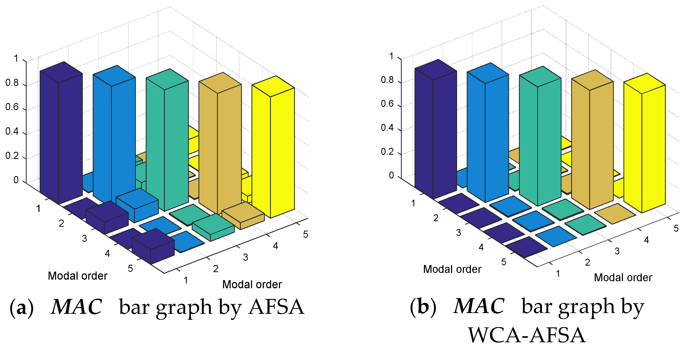
Here, we place 10 WSNs nodes sensors. Figure 8a,b shows the $\mathit{M}\mathit{A}\mathit{C}$ bar graph by AFSA and WCA-AFSA, respectively. Their maximum off-diagonal elements are 0.122655 and 0.008995 respectively. The values of MAC by AFSA and WCA-AFSA are shown in

Table 3. The values of MAC by AFSA.

1	0.003755	0.101833	0.000211	0.122655
0.003755	1	0.113484	0.002971	0.004244
0.101833	0.113485	1	0.008627	0.055712
0.000211	0.002971	0.008627	1	0.058377
0.122655	0.004245	0.055712	0.058377	1

and

Table 4. The values of MAC by WCA-AFSA.

1	0.000093	0.003196	0.000084	0.005940
0.000093	1	0.007748	0.006421	0.000097
0.003196	0.007748	1	0.008995	0.005681
0.000084	0.006421	0.008995	1	0.001002
0.005940	0.000097	0.005681	0.001002	1

. The above result shows that the improved algorithm has better performance.

5.2. Optimal Sensor Placement Scheme

According to engineering practice and test experience, acceleration sensor is usually employed for the monitoring health state of the blade [15]. The scheme of placing 10 WSNs node sensors on the blade is listed in

Table 5. Sensor placement scheme.

Sensor No.	Node No.	Sensor No.	Node No.
1	129	6	633
2	300	7	877
3	861	8	56
4	746	9	741
5	997	10	508

.

The sensors in this placement scheme distribute dispersedly. The scheme avoids the sensors’ local aggregation. Here, sensors are placed in the blade root and other large deformable airfoil locations, which are most in poor conditions. Data from these locations can comprehensively reflect the blade health state.

6. Conclusions

Aiming at the WSN’s node optimal sensor placement for the health monitoring of a wind turbine blade, a weighted centroid fish swarm algorithm is put forward. There are better optimization effects when optimizing the sensor placement of the blade. The conclusions are as follows:

(1)

WCA is introduced to construct the initial fish swarm to enhance the ergodicity of artificial fish optimization and avoid falling into local optimal solution. The fixed step size is improved to the adaptive step size, which speeds up the optimization speed and increases the convergence accuracy.

(2)

WCA-AFSA is used to optimize the WSNs node of the blade. The results show that the WSNs nodes are dispersed, which ensures that the WSNs nodes are located at the most unfavorable position of the blade, and the health information of the blade can be obtained comprehensively.

References

- Oh, K.-Y.; Park, J.-Y.; Lee, J.; Epureanu, B.I. A Novel Method and Its Field Tests for Monitoring and Diagnosing Blade Health for Wind Turbines. IEEE Trans. Instrum. Meas. 2015, 64, 1726–1733. [Google Scholar] [CrossRef]
- Kirikera, G.R.; Shinde, V.; Schulz, M.J.; Ghoshal, A.; Sundaresan, M.J.; Allemang, R.J.; Lee, J.W. A Structural Neural System for Real-time Health Monitoring of Composite Materials. Struct. Health Monit. 2008, 7, 65–83. [Google Scholar] [CrossRef]
- Yick, J.; Mukherjee, B.; Ghosal, D. Wireless sensor network survey. Comput. Netw. 2008, 52, 2292–2330. [Google Scholar] [CrossRef]
- Javadi, M.; Mostafaei, H.; Chowdhurry, M.U.; Abawajy, J.H. Learning automaton based topology control protocol for extending wireless sensor networks lifetime. J. Netw. Comput. Appl. 2018, 122, 128–136. [Google Scholar] [CrossRef]
- Hao, X.C.; Wang, L.Y.; Yao, N.; Geng, D.; Chen, B. Topology control game algorithm based on Markov lifetime prediction model for wireless sensor network. Ad Hoc Netw. 2018, 78, 13–23. [Google Scholar] [CrossRef]
- Chen, L.D. Research on Topology Control of Wireless Sensor Networks; Nanjing University of Posts and Telecommunications: Nanjing, China, 2012. [Google Scholar]
- Naranjo, P.; Shojafar, M.; Mostafaei, H.; Pooranian, Z.; Baccarelli, E. P-SEP: A prolong stable election routing algorithm for energy-limited heterogeneous fog-supported wireless sensor networks. J. Supercomput. 2017, 73, 733–755. [Google Scholar] [CrossRef]
- Ahmadi, A.; Shojafar, M.; Hajeforosh, S.F. An efficient routing algorithm to preserve k -coverage in wireless sensor networks. J. Supercomput. 2014, 68, 599–623. [Google Scholar] [CrossRef]
- Zhu, X.H.; Ni, Z.W.; Cheng, M. Self-adaptive improved artificial fish swarm algorithm with changing step. Comput. Sci. 2015, 42, 210–216. [Google Scholar]
- Li, X.L.; Shao, Z.J.; Qian, J.X. An optimizing method based on autonomous animates: Fish-swarm Algorithm. Syst. Eng. Theory Pract. 2002, 11, 32–38. [Google Scholar]
- Chen, J.; Ge, W.; Tao, L. A weighted compensated localization algorithm of nodes in Wireless Sensor Networks. In Proceedings of the IEEE International Workshop on Advanced Computational Intelligence, Suzhou, China, 25–27 August 2010; pp. 379–384. [Google Scholar]
- Carne, T.G.; Dohrmann, C.R. A Modal Test Design Strategy for Model Correlation. Proc. SPIE Int. Soc. Opt. Eng. 1994, 2460, 927. [Google Scholar]
- Peng, Z.R.; Yin, H.; Pan, A.; Zhao, Y. Chaotic monkey algorithm based optimal sensor placement. Int. J. Control Autom. 2016, 9, 423–434. [Google Scholar] [CrossRef]
- Yu, H.C.; Shi, W.R.; Ran, Q.K.; Wang, K. An Improved Weighted Centroid Location Algorithm Based on Virtual Static Anchor Nodes. Chin. J. Sens. Actuators 2013, 26, 1276–1283. [Google Scholar]
- Gu, G.; Zhao, Y.; Zhang, X. Optimal Layout of Sensors on Wind Turbine Blade Based on Combinational Algorithm. Int. J. Distrib. Sens. Netw. 2016, 2016, 1–8. [Google Scholar] [CrossRef]
© 2018 by the authors. Licensee MDPI, Basel, Switzerland. This article is an open access article distributed under the terms and conditions of the Creative Commons Attribution (CC BY) license (http://creativecommons.org/licenses/by/4.0/).