Fuzzy Q-Learning Agent for Online Tuning of PID Controller for DC Motor Speed Control

Abstract

This paper proposes a hybrid Zeigler-Nichols (Z-N) reinforcement learning approach for online tuning of the parameters of the Proportional Integral Derivative (PID) for controlling the speed of a DC motor. The PID gains are set by the Z-N method, and are then adapted online through the fuzzy Q-Learning agent. The fuzzy Q-Learning agent is used instead of the conventional Q-Learning, in order to deal with the continuous state-action space. The fuzzy Q-Learning agent defines its state according to the value of the error. The output signal of the agent consists of three output variables, in which each one defines the percentage change of each gain. Each gain can be increased or decreased from 0% to 50% of its initial value. Through this method, the gains of the controller are adjusted online via the interaction of the environment. The knowledge of the expert is not a necessity during the setup process. The simulation results highlight the performance of the proposed control strategy. After the exploration phase, the settling time is reduced in the steady states. In the transient states, the response has less amplitude oscillations and reaches the equilibrium point faster than the conventional PID controller.

1. Introduction

DC (Direct Current) motors are used in industries extensively. This is due to their dynamic and reliable behavior. The main aspect of a DC motor is to control its speed. There are three main techniques of controlling the speed of a DC motor. The first one relies on changing the armature resistance, the second one relies on changing the field resistance and the last one relies on changing the armature voltage. The disadvantage of the armature resistance and field circuit techniques is the increase of power losses. Consequently, the best method is the change of the armature voltage [1]. The main method of changing the armature voltage in order to perform speed control in DC motors is the PID. The PID is the most well-known industrial controller, due to its robust performance in a wide range of applications and the ease of implementation. The implementation of a PID controller requires the definition of three parameters, which are the proportional, the integral and the derivative gain. For setting these parameters, there are a variety of methods, mostly empirical, such as Z-N [2]. These methods tune the controller according to the control process, and then the parameters are kept constant, no matter what is happening in the process. This characteristic has many times lead to poor controlling results, due to the dynamic nature of the processes. In these systems, intelligent PID controllers turn out to be very helpful [3] by adopting intelligent techniques such as neural network [4,5,6,7], fuzzy logic [8,9,10], genetic algorithms [11,12,13] etc. Specifically, in terms of speed control of the DC motors, many researchers have been used intelligent PIDs. Supervisor fuzzy controllers have been used for adjusting online the gains of the PID controller in a two-layer control scheme [1,14]. Additionally, neural networks and adaptive neuro-fuzzy inference systems have been used in order to tune online the parameters of the PID controller [15,16]. Genetic algorithms have been used for tuning offline the three terms of the PID controller [17]. These methods require the knowledge of an expert about the process, in order to be embedded in the control scheme. The main disadvantage of these methods lies on cases where there is no information about the process. Additionally, many of them can only optimize the controller offline, and cannot confront changes of the dynamic behavior of the process.

This paper proposes a hybrid Z-N reinforcement learning approach for the online tuning of the parameters of the PID. The PID controller is tuned by the Z-N method, and then its three gains are adapted online through the fuzzy Q-Learning algorithm. This way, the gains of the controller are online adjusted via the interaction with the environment. As a result, the knowledge of an expert is not a necessity during the online tuning process. Q-Learning is a model-free approach and does not require a model of the controlled system. The main advantage of this approach is that it does not require prior knowledge, and its performance is not based on expert knowledge. This happens because its learning mechanism is entirely based on the interaction with the controlled system. On the other hand, Q-Learning is time consuming and needs to explore the state-action space in order to demonstrate good performance. Additionally, it cannot be used in a straight forward manner in problems with continuous state-action space. Recently, Q-Learning has been used in order to improve control processes. In [18], a combination of artificial neural networks and Q-Learning were used for controlling a bioreactor. An artificial neural network controller was trained by data, in order to initialize the Q-function. This way, the exploration phase of the Q-Learning was significantly reduced, and the algorithm converged very quickly. Additionally, in [19] a combination of virtual-reference-feedback-tuning and batch-fitted-Q-Learning approach is applied to a Multi input Multi output nonlinear coupled constrained vertical two-tank system for water level control. In this control scheme, firstly the problem is mostly solved by designing a linear stabilizing virtual-reference-feedback-tuning based feedback controller using few input-output samples from the process in a stable operating point. Next, the resulting controller is used to collect many input-state transition samples from the process in a wide operating range. Finally, a batch fitted Q-Learning strategy uses the database of transition samples to learn a high-performance nonlinear state feedback controller for model reference tracking.

The main contributions of this paper are as follows:

• We deploy a Q-Learning algorithm for adapting online the gains of a PID controller with the initial values that arise by the Z-N method. This PID controller is dedicated to control the speed of a DC motor. This supervision scheme is independent of prior knowledge and is not based on the expert knowledge.
• In order to cope with the continuous state-action space, a fuzzy logic system is used as fuzzy function approximator.

The structure of this paper is as follows: Section 2 provides preliminaries about DC motors, PID controllers, Reinforcement Learning, Q-Learning and fuzzy Q-Learning. Section 3 presents the proposed control scheme. Section 4 presents the experimental results based on the simulated process. Section 5 discusses the experimental results and sketches future work.

2. Preliminaries

2.1. DC Motor

An electric motor converts electric energy to mechanical energy by using interacting magnetic fields. Equation (1) gives the relation between the motor torque and the field current. Equation (2) gives the relation between the armature input voltage and the armature current. Equation (3) describes the relation between back electromotive voltage and motor speed. Equation (4) shows the relation between motor torque and motor speed, Equation (5) gives the model of the DC motor speed system while Equation (6) is the transfer function of the motor speed [20].

$$T_m\left(s\right)=K_T{I}_a\left(s\right)$$

(1)

$$V_a\left(s\right)=\left(R_a+L_{a}s\right)I_a\left(s\right)+V_b\left(s\right)$$

(2)

$$V_b\left(s\right)=K_b\omega \left(s\right)$$

(3)

$$T_m\left(s\right)=J·s·\omega \left(s\right)+b·\omega \left(s\right)$$

(4)

$$\left(Js+b\right)\omega \left(s\right)=K_T\frac{V_a\left(s\right)-K_b\omega \left(s\right)}{\left(R_a+L_{a}s\right)}$$

(5)

$$G\left(s\right)=\frac{K_T}{L_{a}J{s}^2+\left(R_{a}J+L_{a}b\right)s+\left(R_{a}b+K_b{K}_T\right)}$$

(6)

where $T_m$ is the torque of the motor, $K_T$ torque constant, $V_a$ the input voltage, $R_a$ the armature resistance, $L_a$ the armature inductance, $V_b$ the back electromotive force, $K_b$ back electromotive force constant, $\omega$ angular velocity of the motor, $T_L$ load torque, $J$ rotating inertial measurement of motor bearing and $b$ fraction constant.

2.2. PID

The PID controller is a three-term controller. The output of the PID controller depends on the error ($e$) which is the plant output minus the reference signal or set point ($r$) and controls the plant input. The PID control algorithm aims to minimize the error. The proportional gain (kp) is used in order to get the control signal u(t) to respond to the error immediately, so as to increase the system response speed and to reduce steady-state error. The integral gain (ki) is used to eliminate the offset error but causes system response overshoot. In order to reduce the system response overshoot, the derivative gain (kd) is used [21]. The block diagram of a PID controller can be seen in Figure 1 and its transfer function is:

$$G_{PID}\left(s\right)=kp+ki·\frac{1}{s}+kd·s$$

(7)

Figure 1. Block diagram of PID controller.

2.3. Fuzzy Logic Systems (FLS)

Fuzzy logic has the advantage which allows complex processes to be expressed in general terms, without the usage of complex models [22]. The main advantage of fuzzy logic systems is the use of fuzzy if/then rules. These rules embed the knowledge of the expert and can express relations among fuzzy variables using linguistic terms [22]. The generic form of a fuzzy rule is:

$$Ru:\mathit{if}({\mathit{x}}_1\mathrm{is}{D}_1)\mathrm{and}/\mathrm{or}({\mathit{x}}_2\mathrm{is}{D}_2)\dots .\mathrm{and}/\mathrm{or}({\mathit{x}}_m\mathrm{is}{D}_m\left)\mathit{then}\right(c\mathrm{is}E),$$

where $D_j,j=1,\dots ,m$ is a fuzzy set of $j$th input, $\mathit{x}=\left({\mathit{x}}_1,{\mathit{x}}_2,\dots ,{\mathit{x}}_m\right)$ is the crisp input vector, c is the output variable and $E$ is a fuzzy set defined by the expert. The operators “and/or” combine the conditions of the variable inputs that should be satisfied arising the firing strength $w_i\left(\mathit{x}\right)$ of the rule. Two types of FLS are used conventionally, the FLS type Mamdani [23] and the FLS type Sugeno [24]. The main difference between these two types is the way the crisp output is generated; the Mamadani uses a defuzzifier while the Sugeno uses the weighted average [3]. Due to Sugeno’s computational efficiency (lack of defuzzifier), in this paper we are using the zero-order type Sugeno, where the consequents of the rules are constant numbers. The global output of the FLS can be calculated by the Wang-Mendel model [3].

$$a\left(\mathit{x}\right)=\frac{{{\displaystyle \sum }}_{i=1}^N{w}_i\left(\mathit{x}\right)a_i}{{{\displaystyle \sum }}_{i=1}^N{w}_i\left(\mathit{x}\right)}$$

(8)

where $a_i$ is the consequent of rule $i$.

2.4. Reinforcement Learning

Reinforcement learning refers to a family of algorithms inspired by human and animal learning. The objective of this algorithm is to find a policy, i.e., a mapping from states to actions that maximizes the expected discounted reward [25]. This goal is achieved through exploration/exploitation in the space of possible state-action pairs. Actions that share good performance in a given state are given a positive reinforcement signal (reward). Actions leading to poor performance are given a negative reinforcement signal (punishment). Feedback is provided to the system in order to learn the “value” of actions in different states.

2.4.1. Q-Learning

The Q-Learning is a reinforcement learning method. The agent computes the Q-Function, which estimates the future discounted rewards of possible actions applied in states [26]. The output of the Q-Function for a state $\mathit{x}$ and an action $a$ is represented as $Q\left(\mathit{x},a\right)$. The Q value of each action $\mathit{a}$ when performed in a state $\mathit{x}$ can be calculated as follows:

$$Q^{\prime }\left(\mathit{x},a\right):=Q\left(\mathit{x},a\right)+\eta \left(R\left(\mathit{x},a,{\mathit{x}}^{\prime }\right)+\gamma {}_a{}^{max}Q\left({\mathit{x}}^{\prime },a\right)-Q\left(\mathit{x},a\right)\right)$$

(9)

where $Q^{\prime }\left(\mathit{x},a\right)$ is the updated value of the state-action combination when the agent obtains the reward $R\left(\mathit{x},a,{\mathit{x}}^{\prime }\right)$ after executing the action $a$ in the state $\mathit{x}$. Q-Learning assumes that the agent continues for state $\mathit{x}$ by performing the optimal policy, thus ${}_a{}^{ma\mathit{x}}Q\left({\mathit{x}}^{\prime },a\right)$ is the maximum value of the execution of the best action in the state ${\mathit{x}}^{\prime }$ (the state comes out after performing $a$ in state $\mathit{x}$). The learning rate $\eta$ defines in which degree the new information overrides the old one [27]. The discount factor $\gamma$ defines the significance of the future rewards [28]. Overall, the Q-Learning agent chooses the action $a$ to be applied in the current state $\mathit{x}$ and identifies the next state ${\mathit{x}}^{\prime }$. It acquires the reward from this transition i.e., $R\left(\mathit{x},a,{\mathit{x}}^{\prime }\right)$, and updates the value for the pair $\left(\mathit{x},a\right)$ assuming that it performs the optimal policy from state $\mathit{x}$ and on. A Q-Learning agent applies an exploration/exploitation scheme in order to compute a policy that maximizes the sum of future discounted rewards ($REW$).

$$REW={\displaystyle \sum }_{i=0}^t{\gamma }^{\iota }{R}_i$$

(10)

where $t$ is the number of the time steps. The main characteristic which makes Q-Learning suitable to be applied in our study is its model-free approach. On the other hand, Q-Learning cannot be applied in a straightforward manner to the continuous action-state spaces that our problem involves. The simplest solution in order for Q-Learning to be applied in continuous action-state spaces is to discretize the action-state space. Discretizing the space may lead to sudden changes in actions, even for smooth changes in states. Making the discretization more fine-grained will smooth these changes, but the state-action combination increases. In problems with multidimensional state space, the number of the combinations grows exponentially. On the other hand, by using other approximators such as neural networks, two slow processes are combined. Q-Learning and neural networks are known for their slow learning rate [29]. In order to overcome these limitations, fuzzy function approximation can be used in combination with Q-Learning, as fuzzy systems are universal approximators [30]. Knowledge of the expert can be embedded in order to assist the learning mechanism. Through this method, actions change smoothly in response to smooth changes in states, without the need for discretizing the space in a fine-grained way [31].

2.4.2. Fuzzy Q-Learning

In Q-Learning, Q-values are stored and updated for each state-action pair. In cases where the number of state-action pairs is very large, the implementation might be impractical. Fuzzy Inference Systems have the advantage of achieving good approximations [32] in the Q-function, and simultaneously make possible the use of the Q-Learning in continuous states-space problems (Fuzzy Q-Learning) [29]. In fuzzy Q-Learning, $\mathit{x}$ is the crisp set of the inputs defining the state of the agent. These are converted into fuzzy values and each fuzzy rule corresponds to a state. In other words, the firing strength of each rule defines the degree to which the agent is in a state. Furthermore, the rules do not have fixed consequents; meaning there are no fixed (predefined) state-action pairs but through the exploration/exploitation algorithm arise the consequents of each rule (state-action pair). Thus, the FIS has competing actions for each rule and the rules have the form:

$$\begin{array}{ccc}\mathit{if}\mathit{x}is{S}_i& \mathit{then}& \alpha \left[i,1\right]\\ & \mathrm{or}& \alpha \left[i,2\right]\\ & ⋮& \\ & \mathrm{or}& \alpha \left[i,k\right]\end{array}$$

where $\alpha \left[i,k\right]$ is the kth possible action in rule $i$. For each possible action in rule $i$ there is a corresponding value $q\left[i,k\right]$. This corresponding value determines how “good” the corresponding action is, when the rule $i$ is fired. The state $S_i$ is defined by $\left(x_{1}is{S}_{i,1}and{x}_{2}is{S}_{i,2}\dots and{x}_{n}is{S}_{i,n}\right)$, where $S_{i,j}$, $j=1,\dots ,n$ are fuzzy sets. Specifically, the algorithm of the fuzzy Q-Learning is briefly presented below.

• Observe state $\mathit{x}$
• Take an action ${\alpha }_i$ for each rule $i$ according to exploration/exploitation algorithm
• Calculate the global output $a\left(\mathit{x}\right)$ according to Equation (10)
• Calculate the corresponding value $Q\left(\mathit{x},a\right)$ according to Equation (11)
• Capture the new state information
• Calculate reward $R\left(\mathit{x},a,{\mathit{x}}^{\prime }\right)$
• Update q-values according to Equation (12)

The fuzzy Q-Learning algorithm and its equation are described extensively in seven steps.

(1)

Observation of the state $\mathit{x}$

(2)

For each fired rule, one action is selected according to the exploration/exploitation strategy.

(3)

Calculation of the global output $a\left(\mathit{x}\right)$

$$a\left(\mathit{x}\right)=\frac{{{\displaystyle \sum }}_{i=1}^N{w}_i\left(\mathit{x}\right)a_i}{{{\displaystyle \sum }}_{i=1}^N{w}_i\left(\mathit{x}\right)}$$

(11)

where $a_i$ is as specified in Section 2.4.2 (consequents of the rule $i$) and corresponds to the selected action of rule $i$.

(4)

Calculation of the corresponding value $Q\left(\mathit{x},a\right)$.

$$Q\left(\mathit{x},a\right)=\frac{{{\displaystyle \sum }}_{i=1}^N{w}_i\left(\mathit{x}\right)a_{i}q\left[i,i^{†}\right]}{{{\displaystyle \sum }}_{i=1}^N{w}_i\left(\mathit{x}\right)}$$

(12)

where $q\left[i,i^{†}\right]$ is the corresponding q-value of the fired rule $i$ for the selection of the action $i^{†}$ by the exploration algorithm.

(5)

Application of the action $a\left(\mathit{x}\right)$ and observation of the new state ${\mathit{x}}^{\prime }$.

(6)

Calculation of the reward $R\left(\mathit{x},a,{\mathit{x}}^{\prime }\right)$.

(7)

Updating the q values according to:

$$\Delta q\left[i,i^{†}\right]=\eta \Delta Q\frac{w_i\left(\mathit{x}\right)}{{{\displaystyle \sum }}_{i=1}^N{w}_i\left(\mathit{x}\right)}$$

(13)

where $\Delta Q=R\left(\mathit{x},a,{\mathit{x}}^{\prime }\right)+\gamma ·Q\left({\mathit{x}}^{\prime },a^{*}\right)-Q\left(\mathit{x},a\right)$, $Q\left({\mathit{x}}^{\prime },a^{*}\right)=\frac{{{\displaystyle \sum }}_{i=1}^N{w}_i\left({\mathit{x}}^{\prime }\right)a_{i}q\left[i,i^{*}\right]}{{{\displaystyle \sum }}_{i=1}^N{w}_i\left({\mathit{x}}^{\prime }\right)}$ and $q\left[i,i^{*}\right]$ is the selection of the action $i^{*}$ that has the maximum Q value for the fired rule $i$.

3. Control Strategy

The block diagram of the control strategy is depicted in Figure 2. The set point ($r$) is the desired angular velocity of the rotor. The measured value of the rotor velocity, through the feedback control loop, is subtracted from the set point and the value of the error (e) arises. The error is the input of both the PID controller and the fuzzy Q-Learning agent. The PID gains are set offline by the Z-N method and then they are tuned online by the fuzzy Q-Learning algorithm. The control process is the speed of the motor, which has as input the control signal of the PID controller (voltage) and as output the angular velocity of the rotor.

Figure 2. Block diagram of the control strategy.

The parameters of the DC motor can be seen in Table 1.

Table 1. Motor parameters.

Parameter	Value
$J$	$0.0113\mathrm{N}·\mathrm{m}·{\mathrm{s}}^2/\mathrm{rad}$
$b$	$0.028\mathrm{N}·\mathrm{m}·\mathrm{s}/\mathrm{rad}$
$L_a$	$0.1\mathrm{H}$
$R_a$	$0.45\mathsf{\Omega }$
$K_T$	$0.067\mathrm{N}·\mathrm{m}/\mathrm{A}$
$K_b$	$0.067\mathrm{V}·\mathrm{s}/\mathrm{rad}$

The transfer function of the given motor is:

$$G\left(s\right)=\frac{0.067}{0.00113{\mathrm{s}}^2+0.0078854\mathrm{s}+0.0171}$$

(14)

and the transfer function of the PID controller tuning by the Z-N method is:

$$G_{PID}\left(s\right)=2.42+14.89\frac{1}{s}+0.1s$$

(15)

More information about the DC motor model and the transfer function of the PID controller can be found in [20].

The input signal (error) of the fuzzy Q-Learning agent defines the value of its only one state variable and is conditioning in the range of [–1, 1]. For this input, we use seven Membership Functions (MFs) (Figure 3). The PB, PM, PS, Z, NS, NM and NB denote Positive Big, Positive Medium, Positive Small, Zero, Negative Small, Negative Medium and Negative Big, respectively. The one input with the seven MF’s results to 7 states represented by an equal number of fuzzy rules.

Figure 3. Input membership functions.

The output of the agent is a vector with three output variables, $A=[A^p{A}^i{A}^d]$ each one for each gain of the PID controller. Each output variable has a group of five fuzzy actions (fuzzy singletons). For the output variable $A^p$ the group of the fuzzy singletons is: $A^p=\left\{\frac{1}{-0.5}+\frac{1}{-0.25}+\frac{1}{0}+\frac{1}{0.25}+\frac{1}{0.5}\right\}$. Where “+” is the union operator and “−” denotes a membership degree to a value of the membership function domain. For the output variable $A^i$ the group of the fuzzy singletons is: $A^i=\left\{\frac{1}{-0.5}+\frac{1}{-0.25}+\frac{1}{0}+\frac{1}{0.25}+\frac{1}{0.5}\right\}$ and for the output variable $A^d$ the group of the fuzzy singletons is: $A^p=\left\{\frac{1}{-0.5}+\frac{1}{-0.25}+\frac{1}{0}+\frac{1}{0.25}+\frac{1}{0.5}\right\}$. Each value of the output variable represents the percentage change of each gain according to its initial value, which has arisen by the Z-N method. The action space of the agent consists of 125 actions and the total state-action space consists of 875 combinations.

As mentioned before, the agent learns through the interaction of the environment. In order to acquire knowledge through its experience, an exploration/exploitation algorithm must be used in order to define whether the agent is to perform exploration or exploitation. In order to perform high exploration when the agent goes to a new state, agents explore for a certain number of rounds per state (500 rounds/state). The agent then checks and performs the action that has not been performed at all (if there are any). This allows all possible actions to be performed at least one time for each state. After that, the agent performs exploitation for 99% and 1% exploration for a given state.

The agent reward ($R$) is defined as follows:

$$R=\frac{1}{1+\left|e^{\prime }\right|}-\frac{1}{1+\left|e\right|}$$

(16)

where $e^{\prime }$ is the error in the next state. The fraction $\frac{1}{1+\left|e\right|}$ takes value in the range [0, 1]. If the value of the error is zero, the value of this quantity becomes “1”. On the other hand, high positive or negative values of error reduce this quantity. The result of subtracting this quantity with the quantity which has the error in the next state, gives a reward which can take positive and negative values. Positive values indicate that the error in the next state is reduced. Negative values indicate that the error in the next state is raised. Higher values of reward indicate higher reduction of the error and vice versa. The sum of future discounted rewards in this problem is defined as:

$$REW={\displaystyle \sum }_{i=0}^t{\gamma }^{\iota }(\frac{1}{1+\left|e_i\right|}-\frac{1}{1+\left|e_{(i-1)}\right|})$$

(17)

4. Simulation Results

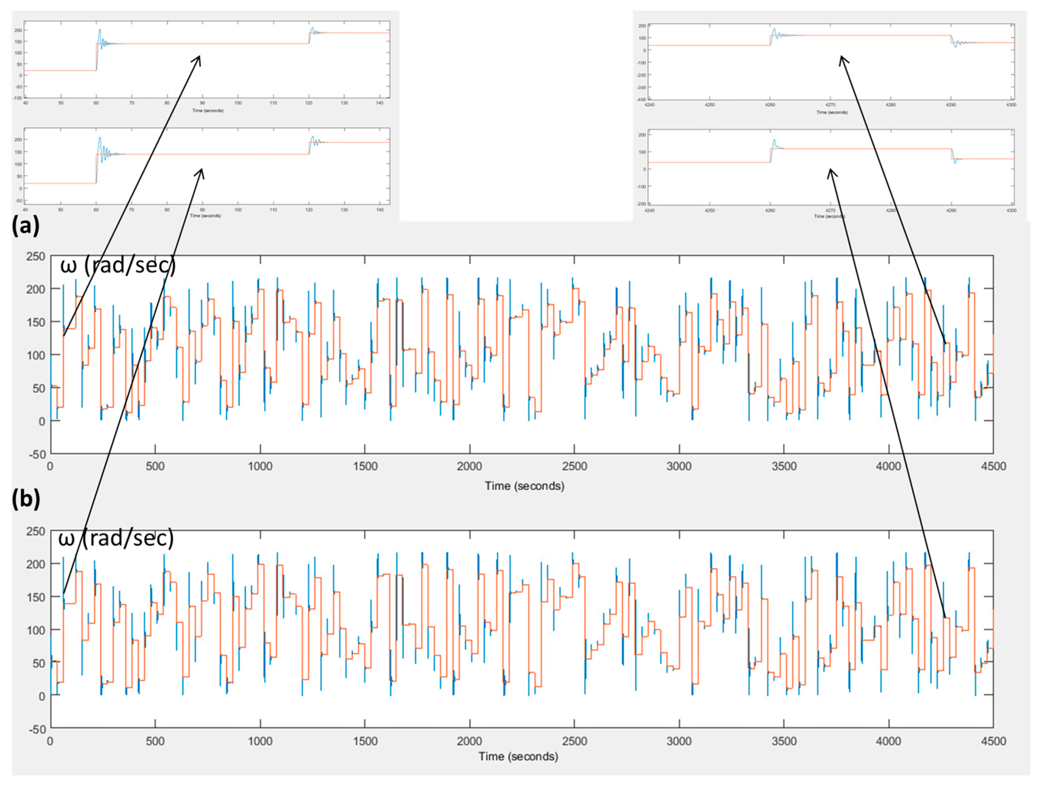
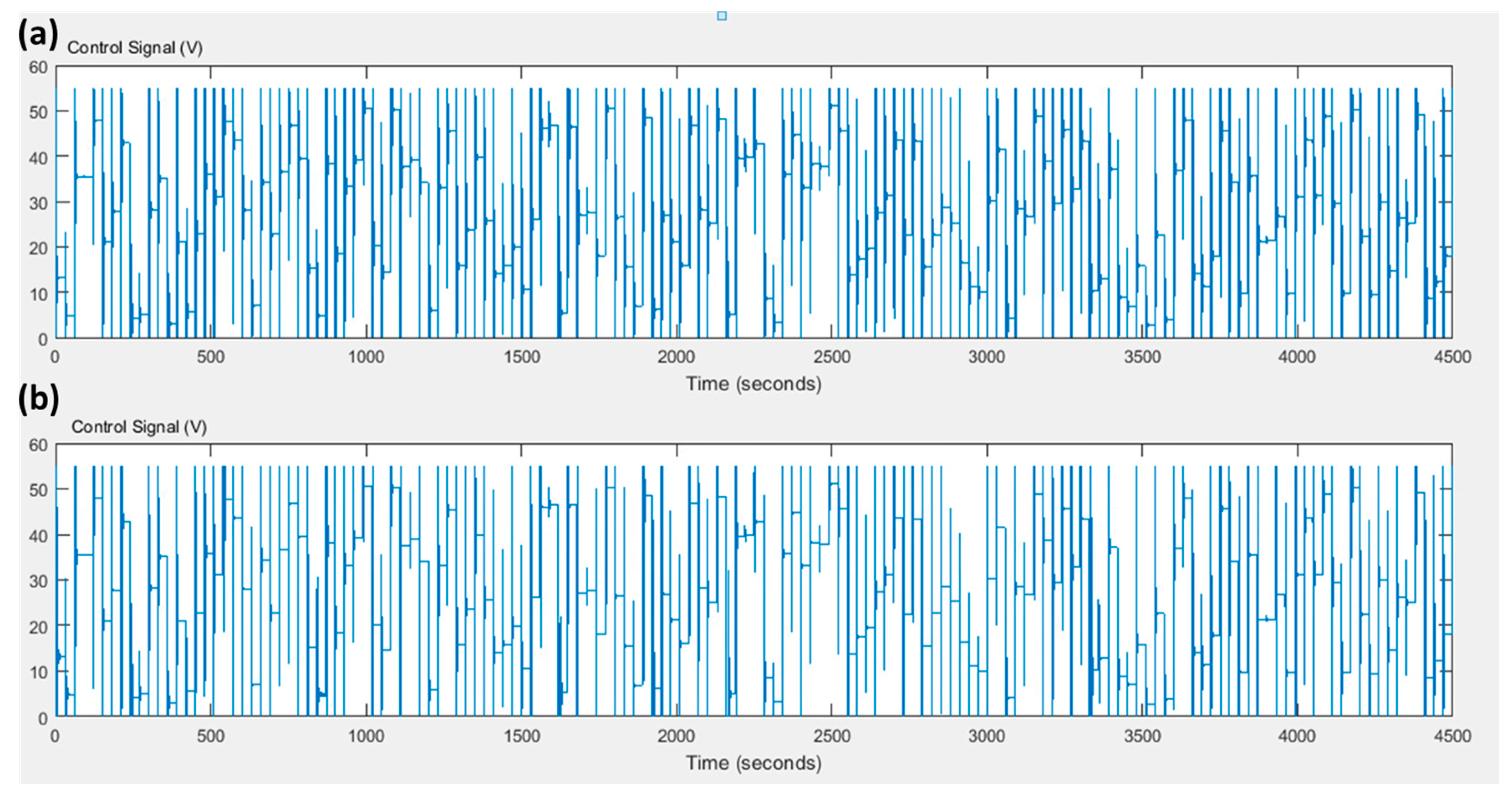
The simulation will compare the conventional PID tuned by Z-N with the proposed method. This comparison aims to highlight the improvement of the conventional PID through the supervision of the fuzzy Q-Learning algorithm. The simulation time is set to 4500 s with a simulation step time of 0.001 s. The round of the fuzzy Q-Learning agent is 0.1 s. The value of the learning rate and the discount factor equals to $\eta =0.1$ and $\gamma =0.9$ respectively. During the simulation, various set points are applied in the range of [10, 250] rad/s with sample time of 30 s. Figure 4 presents the set point of the motor’s velocity; the velocity of the motor which is controlled by the conventional PID controller, tuned by the Z-N method and by the fuzzy Q-Learning PID controller. Figure 5 presents the control signal of both controllers. In the beginning of the simulation, where the fuzzy Q-Learning agent mainly explores, we can see that the rising time is the same for both controllers. On the contrary, the fuzzy Q-Learning PID controller increases the amplitude of the oscillations in the transient states, and it also increases the settling time. During the exploitation phase, we can see that the fuzzy Q-Learning PID controller performs better. The rising time is again the same for both controllers, but now the oscillations of the fuzzy Q-Learning PID have lower amplitude values in the transient states and the settling time is less compared to the conventional PID controller. Characteristics of the output response for both controllers can be found in Table 2 for two different time points. These two points are at 60 s (exploration phase) and at 4260 s (exploitation phase).

Figure 4. (a) Velocity of DC motor (ω) with conventional PID control strategy (blue line) and velocity set point (red line), and (b) velocity of DC motor (ω) with fuzzy Q-Learning PID control strategy (blue line) and velocity set point (red line).

Figure 5. (a) Control signal of conventional PID control strategy and (b) control signal of fuzzy Q-Learning PID control strategy.

Table 2. Performance characteristics.

Characteristic	Step Response at 60 s		Step Response at 4260 s
	PID Z-N	Fuzzy Q-Learning PID	PID Z-N	Fuzzy Q-Learning PID
Settling time (s)	3.30	4.05	3.67	1.72
Rising time (s)	0.35	0.35	0.27	0.27
Overshoot (%)	54.2	58.3	71.0	67.5

The better performance of the fuzzy Q-Learning PID after the exploration phase is also indicated by the values of the Integral Absolute Error ($IAE$) and the Integral Time Absolute Error ($ITAE$). The $IAE$ and the $ITAE$ are defined as:

$$IAE=\int \left|e\right|dt$$

(18)

$$\mathrm{ITAE}\int t\left|e\right|dt$$

(19)

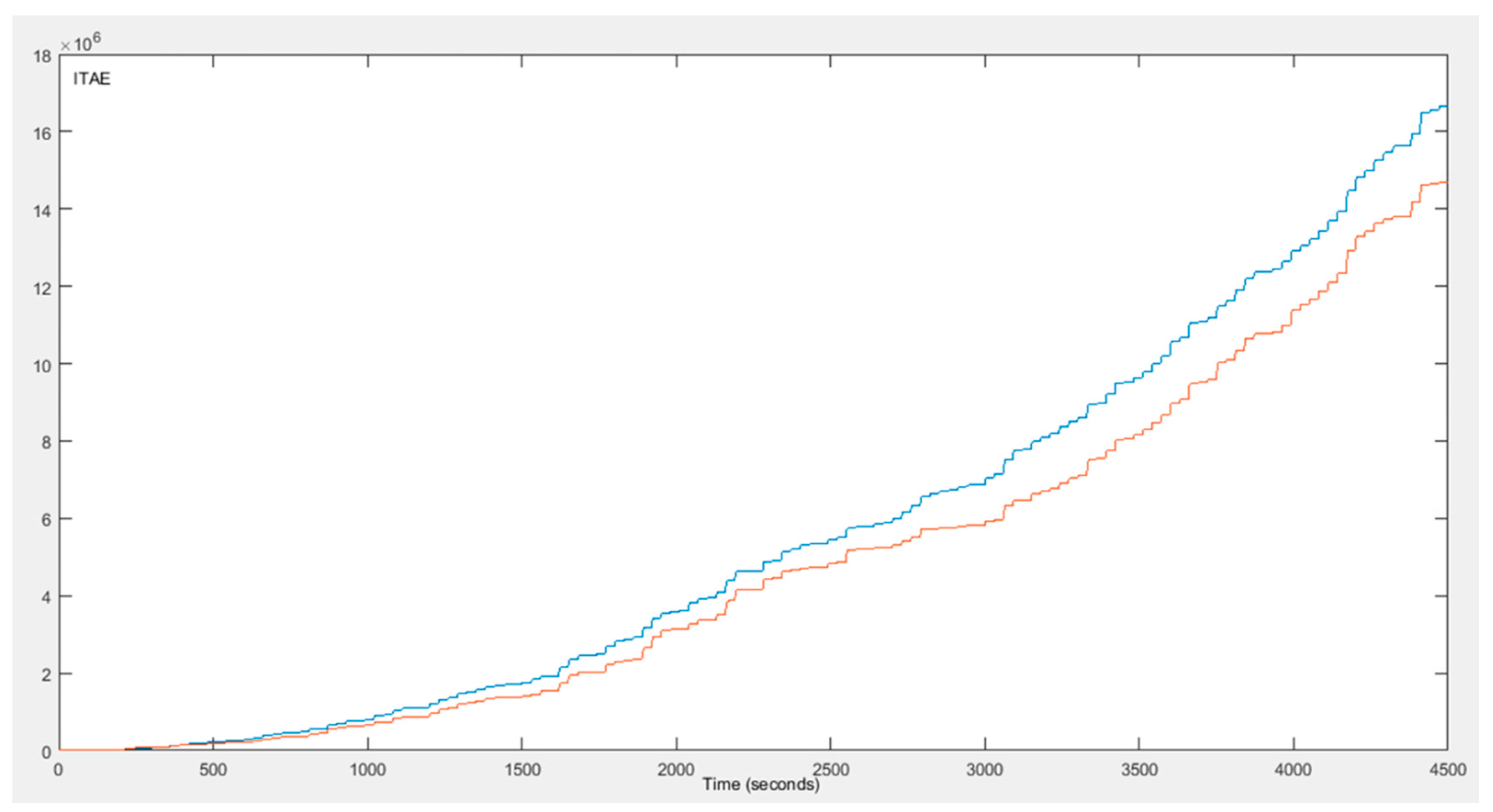
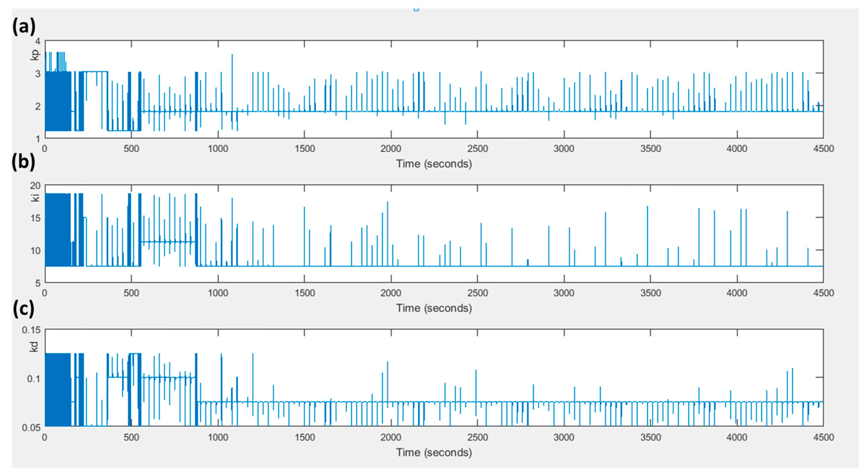
At this point, it is worth mentioning that maximizing the value of $REW$ does not mean that the values of $IAE$ and ITAE are minimized. Both the values of the $IAE$ and the $ITAE$ are minimized when the error is zero. If the values of the error in both states are set to zero, then the value of the $REW$ is not maximized but becomes zero. On the other hand, when the value of the error in the current state is very big and the value of the error in the next state is zero, the value of the $REW$ is maximized, while the $IAE$ and the $ITAE$ are not minimized. Figure 6 and Figure 7 present the values of $IAE$ and $ITAE$ for both control strategies through time. It is obvious that the conventional PID performs better in the beginning ($IAE$ and $ITAE$ have lower values), but as the agent of the fuzzy Q-Learning PID controller turns from the exploration to exploitation, the values of the $IAE$ and $ITAE$ turn to be lower. Finally, Figure 8 presents how the three gains of the proposed control strategy are changed through time in respect to the various changes of the set point.

Figure 6. $IAE$ of conventional PID control strategy (blue line) and fuzzy Q-Learning PID control strategy (red line).

Figure 7. $ITAE$ of conventional PID control strategy (blue line) and fuzzy Q-Learning PID control strategy (red line).

Figure 8. Values of (a) kp, (b) ki and (c) kd through the simulation.

5. Discussion

This paper demonstrates a fuzzy Q-Learning agent for tuning online the gains of a PID controller, which is used to control the speed of a DC motor. The initial values of the controller’s gains have been arisen from the Z-N method. The Q-Learning agent has as input variable, the error, and as output variables, the percentage changes of the gains. Fuzzy logic is combined with Q-Learning algorithm in order to deal with the continuous state-action space as the conventional Q-Learning algorithm can be applied to discrete state-action space.

When a fuzzy Q-Learning agent is designed, three main points need to be taken into consideration. The first point lies on the selection of the state variables. A state should be descriptive enough in order to describe the conditions of the system, but without redundant information which will lead to a very large state space. The second point lies on the definition of the reward. The reward must be accurate enough in order for the algorithm to converge quickly and accurately. Last but not least, the exploration/exploitation algorithm has to be chosen in dependence to the nature of the environment (stochastic, deterministic, single agent, multiagent, etc.) in order for the algorithm to converge quickly by exploring the possible paths.

The fuzzy Q-Learning agent learns by interacting with the environment, and the total control strategy indicates a better performance than the conventional PID controller. The simulation results highlight this performance, as both the amplitude of the oscillations and the settling time are reduced. Additionally, the values of the IAE and the ITAE confirm the better performance.

In future, it is our aim to add another state variable (change of error) in the fuzzy Q-Learning algorithm to enhance the performance of the agent. On the other hand, this addition will increase exponentially the state-action space and extensive exploration will be needed. Thus, it would be prudent to turn to multiagent system approaches in order to decompose the problem and reduce the state-action space.

References

- Akbari-Hasanjani, R.; Javadi, S.; Sabbaghi-Nadooshan, R. DC motor speed control by self-tuning fuzzy PID algorithm. Trans. Inst. Meas. Control 2015, 37, 164–176. [Google Scholar] [CrossRef]
- Meshram, P.M.; Kanojiya, R.G. Tuning of PID Controller using Ziegler-Nichols Method for Speed Control of DC Motor. In Proceedings of the IEEE International Conference on Advances in Engineering, Science and Management (ICAESM-2012), Nagapattinam, Tamil Nadu, India, 30–31 March 2012. [Google Scholar]
- Wang, L.-X. A Course in Fuzzy Systems and Control; Prentice Hall PTR: Upper Saddle River, NJ, USA, 1997. [Google Scholar]
- Liu, L.; Luo, J. Research of PID Control Algorithm Based on Neural Network. Energy Procedia 2011, 13, 6988–6993. [Google Scholar]
- Badr, A.Z. Neural Network Based Adaptive PID Controller. IFAC Proc. Vol. 1997, 30, 251–257. [Google Scholar] [CrossRef]
- Rad, A.B.; Bui, T.W.; Li, V.; Wong, Y.K. A new on-line PID tuning method using neural networks. IFAC Proc. Vol. 2000, 33, 443–448. [Google Scholar] [CrossRef]
- Du, X.; Wang, J.; Jegatheesan, V.; Shi, G. Dissolved Oxygen Control in Activated Sludge Process Using a Neural Network-Based Adaptive PID Algorithm. Appl. Sci. 2018, 8, 261. [Google Scholar] [CrossRef]
- Muhammad, Z.; Yusoff, Z.M.; Kasuan, N.; Nordin, M.N.N.; Rahiman, M.H.F.; Taib, M.N. Online Tuning PID using Fuzzy Logic Controller with Self-Tuning Method. In Proceedings of the IEEE 3rd International Conference on System Engineering and Technology, Shah Alam, Malaysia, 19–20 August 2013. [Google Scholar]
- Dounis, A.I.; Kofinas, P.; Alafodimos, C.; Tseles, D. Adaptive fuzzy gain scheduling PID controller for maximum power point tracking of photovoltaic system. Renew. Energy 2013, 60, 202–214. [Google Scholar] [CrossRef]
- Qin, Y.; Sun, L.; Hua, Q.; Liu, P. A Fuzzy Adaptive PID Controller Design for Fuel Cell Power Plant. Sustainability 2018, 10, 2438. [Google Scholar] [CrossRef]
- Amaral, J.F.M.; Tanscheit, R.; Pacheco, M.A.C. Tuning PID Controllers through Genetic Algorithms. In Proceedings of the 2001 WSES International Conference on Evolutionary Computation, Puerto De La, Spain, 11–15 February 2001. [Google Scholar]
- Jayachitra, A.; Vinodha, R. Genetic Algorithm Based PID Controller Tuning Approach for Continuous Stirred Tank Reactor. Adv. Artif. Intell. 2014, 2014, 9. [Google Scholar] [CrossRef]
- Sheng, L.; Li, W. Optimization Design by Genetic Algorithm Controller for Trajectory Control of a 3-RRR Parallel Robot. Algorithms 2018, 11, 7. [Google Scholar] [CrossRef]
- Jigang, H.; Jie, W.; Hui, F. An anti-windup self-tuning fuzzy PID controller for speed control of brushless DC motor. J. Control Meas. Electron. Comput. Commun. 2017, 58, 321–335. [Google Scholar] [CrossRef]
- Zhang, S.M.; Zhou, X.; Yang, L. Adaptive PID regulator based on neural network for DC motor speed control. In Proceedings of the International Conference on Electrical and Control Engineering, Yichang, China, 16–18 September 2011. [Google Scholar]
- Ji, H.; Li, Z. Design of Neural Network PID Controller Based on Brushless DC Motor. In Proceedings of the Second International Conference on Intelligent Computation Technology and Automation, Changsha, China, 10–11 October 2011. [Google Scholar]
- Elsrogy, W.M.; Fkirin, M.A.; Hassan, M.A.M. Speed Control of DC Motor Using PID Controller Based on Artificial Intelligence Techniques. In Proceedings of the International Conference on Control, Decision and Information Technologies, Hammamet, Tunisia, 6–8 May 2013. [Google Scholar]
- Pandian, B.J.; Noel, M.M. Control of a bioreactor using a new partially supervised reinforcement learning algorithm. J. Process Control 2018, 69, 16–29. [Google Scholar] [CrossRef]
- Radac, M.-B.; Precup, R.-E.; Roman, R.-C. Data-driven model reference control of MIMO vertical tank systems with model-free VRFT and Q-Learning. ISA Trans. 2018, 73, 227–238. [Google Scholar] [CrossRef] [PubMed]
- Abdulameer, A.; Sulaiman, M.; Aras, M.S.M.; Saleem, D. Tuning Methods of PID Controller for DC Motor Speed Control. Indones. J. Electr. Eng. Comput. Sci. 2016, 3, 343–349. [Google Scholar] [CrossRef]
- Bhagat, N.A.; Bhaganagare, M.; Pandey, P.C. DC Motor Speed Control Using PID Controllers; EE 616 Electronic System Design Course Project; EE Dept., IIT Bombay: Mumbai, India, November 2009. [Google Scholar]
- Tsoukalas, L.H.; Uhring, R.E. Fuzzy and Neural Approaches in Engineering, 1st ed.; John Wiley & Sons, Inc. Press: New York, NY, USA, 1996. [Google Scholar]
- Mamdani, E.H.; Assilian, S. An experiment in linguistic synthesis with a fuzzy logic controller. Int. J. Man-Mach. Stud. 1975, 7, 1–13. [Google Scholar] [CrossRef]
- Takagi, T.; Sugeno, M. Fuzzy identification of systems and its applications to modeling and control. IEEE Trans. Syst. Man Cybern. 1985, 15, 116–132. [Google Scholar] [CrossRef]
- Russel, S.; Norving, P. Artificial Intelligence: A Modern Approach; Prentice Hall PTR: Upper Saddle River, NJ, USA, 1995. [Google Scholar]
- Watkins, C.J.C.H. Learning from Delayed Reinforcement Signals. Ph.D. Thesis, University of Cambridge, Cambridge, UK, 1989. [Google Scholar]
- Sutton, R.; Barto, A. Reinforcement Learning: An Introduction; MIT Press: Cambridge, MA, USA, 1998. [Google Scholar]
- François-Lavet, V.; Fonteneau, R.; Ernst, D. How to Discount Deep Reinforcement Learning: Towards New Dynamic Strategies. arXiv, 2015; arXiv:1512.02011. [Google Scholar]
- Glorennec, P.Y.; Jouffe, L. Fuzzy Q-Learning. In Proceedings of the 6th International Fuzzy Systems Conference, Barcelona, Spain, 5 July 1997; pp. 659–662. [Google Scholar]
- Wang, L.X. Fuzzy Systems are Universal approximators. In Proceedings of the First IEEE Conference on Fuzzy System, San Diego, CA, USA, 8–12 March 1992; pp. 1163–1169. [Google Scholar]
- Van Hasselt, H. Reinforcement Learning in Continuous State and Action Spaces. In Reinforcement Learning: State of the Art; Springer: Berlin, Heidelberg, 2012; pp. 207–251. [Google Scholar]
- Castro, J.L. Fuzzy logic controllers are universal approximators. IEEE Trans. Syst. Man Cybern. 1995, 25, 629–635. [Google Scholar] [CrossRef] [Green Version]
Figure 1.
Block diagram of PID controller.
Figure 2.
Block diagram of the control strategy.
Figure 3.
Input membership functions.
Figure 4.
(a) Velocity of DC motor (ω) with conventional PID control strategy (blue line) and velocity set point (red line), and (b) velocity of DC motor (ω) with fuzzy Q-Learning PID control strategy (blue line) and velocity set point (red line).
Figure 5.
(a) Control signal of conventional PID control strategy and (b) control signal of fuzzy Q-Learning PID control strategy.
Figure 6.
of conventional PID control strategy (blue line) and fuzzy Q-Learning PID control strategy (red line).
Figure 7.
Figure 8.
Values of (a) kp, (b) ki and (c) kd through the simulation.