A New Greedy Insertion Heuristic Algorithm with a Multi-Stage Filtering Mechanism for Energy-Efficient Single Machine Scheduling Problems

Abstract
:1. Introduction
2. MILP Formulation for the Problem
3. A Greedy Insertion Heuristic Algorithm with Multi-Stage Filtering Mechanism
3.1. The Characteristics of TOU Electricity Tariffs
3.2. Multi-Stage Filtering Mechanism Design
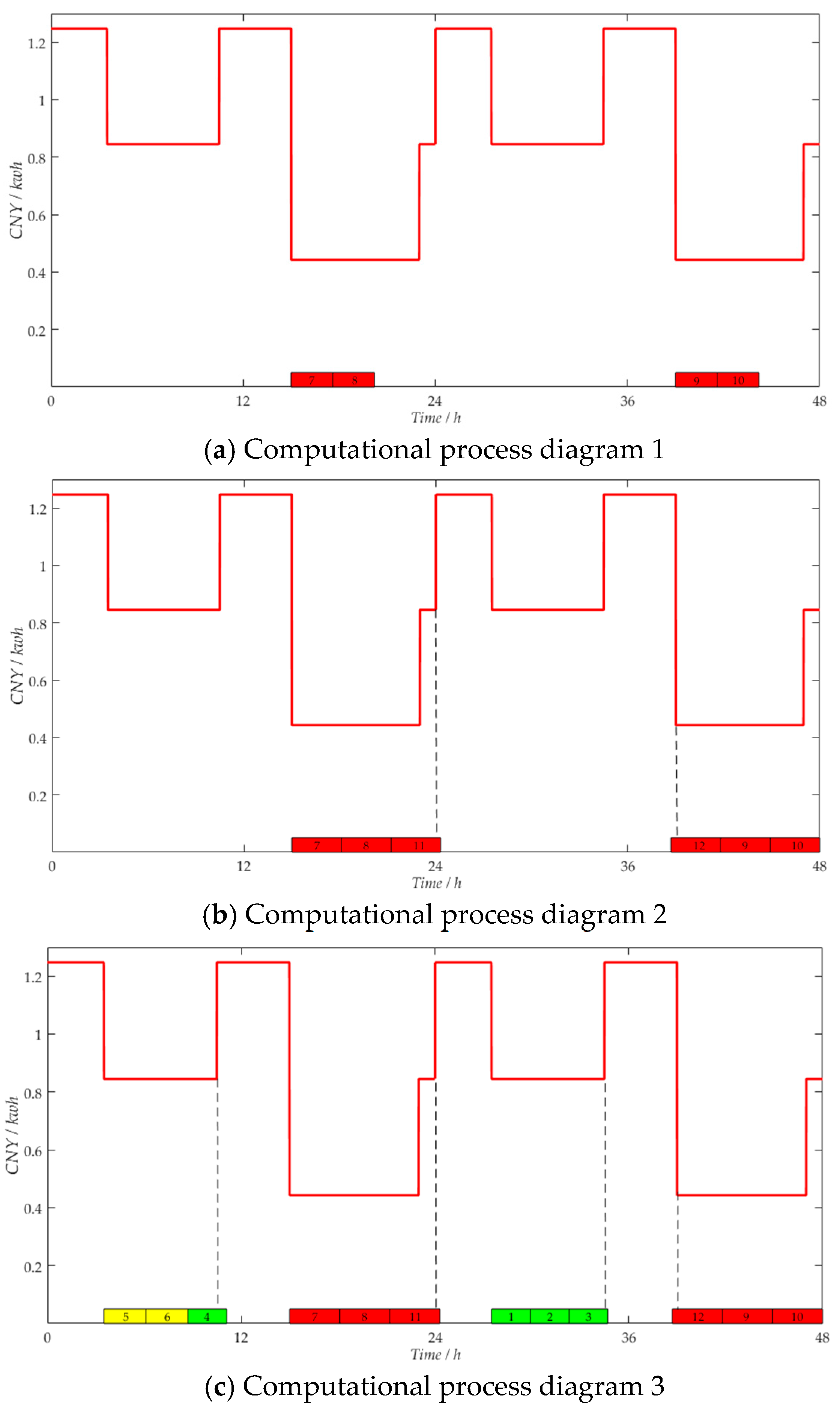
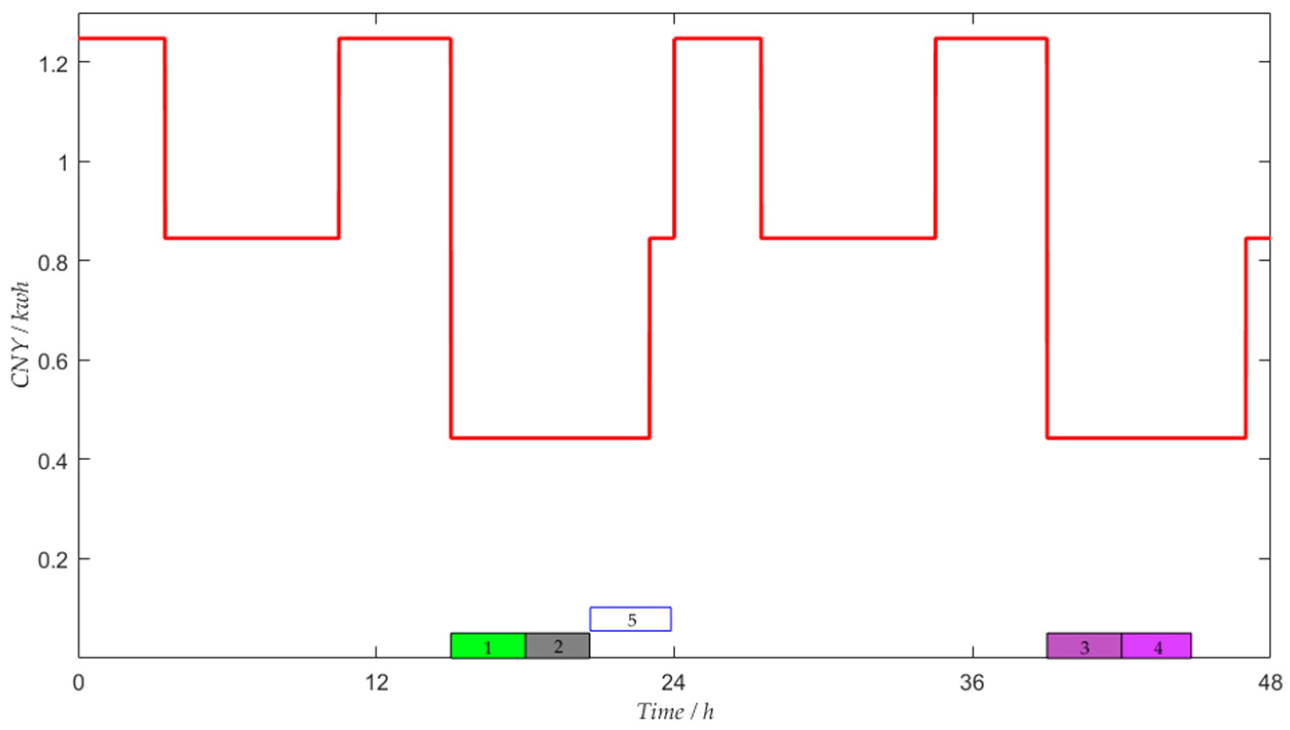
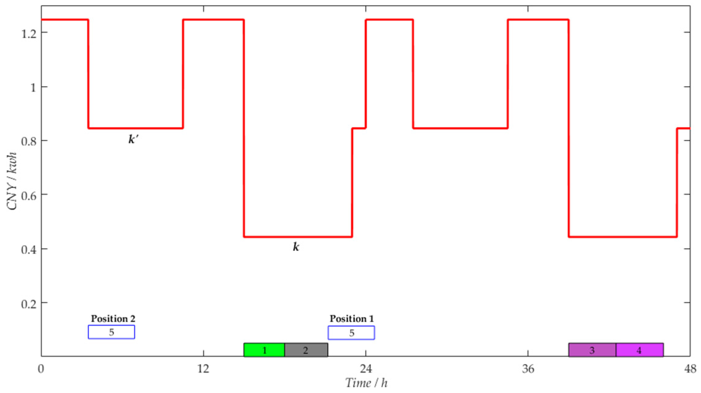
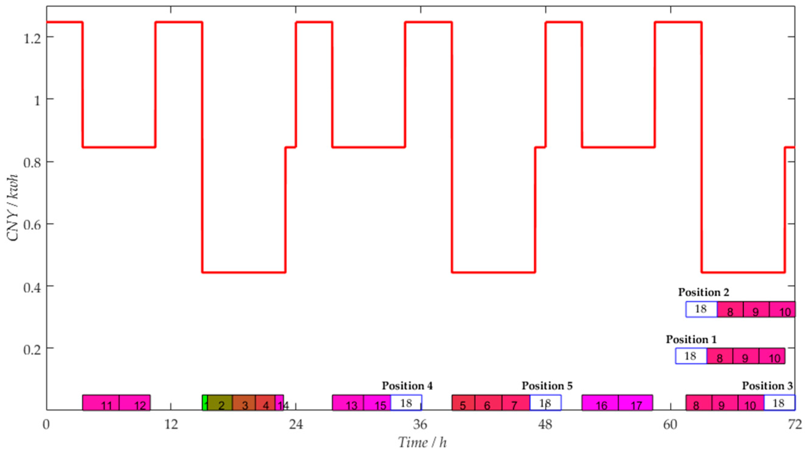
- To occupy off-peak periods as much as possible, a set of already inserted jobs in period k should be moved to the rightmost side, and then job i can be processed across periods k and k − 1.
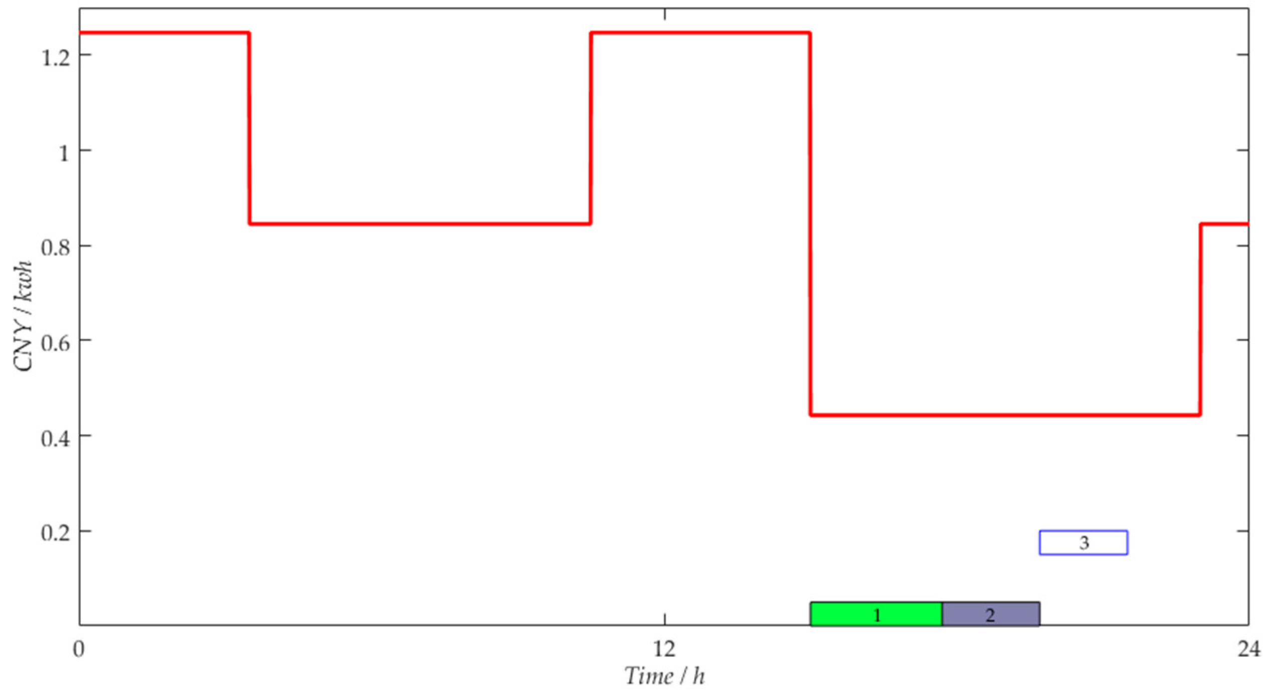
- All inserted jobs in period k should be moved left so that job i can be processed within period k.
- 3.
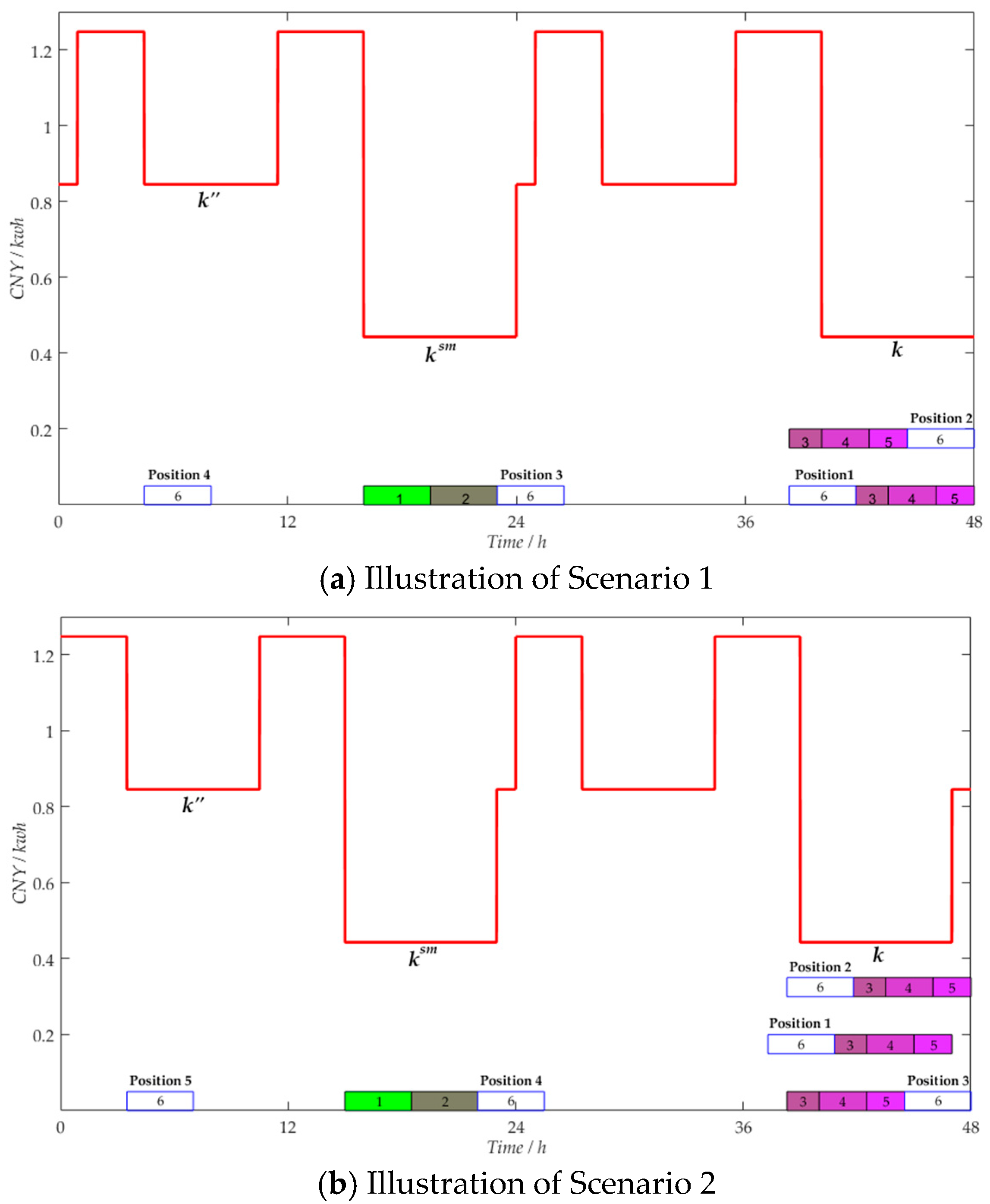
- Suppose that job i is processed across periods ksm, ksm + 1, and ksm + 2. If Iksm is slightly smaller than Ik, cost3 may be less than cost1 as period ksm + 1 is a mid-peak period. Hence, Position 3 needs to be considered.
- 4.
- Similar to Condition 3, job i can be processed within a mid-peak period.
- A set of already inserted jobs in period k are moved to the rightmost side of the period k + 1, and then job i is processed across periods k and k − 1.
- A set of already inserted jobs in period k should be moved to the left until job i can be processed across periods k and k + 1.
| Algorithm 1: Greedy insertion heuristic algorithm with multi-stage filtering mechanism |
| 1. Sort all jobs in non-increasing order of their power consumption rates 2. Initialization: Ik = bk+1 − bk, for all 1 ≤ k ≤ m 3. For i = 1 to n do 3.1. If layer 1 C1. If Condition 1 is satisfied Initial the period index //Job i is processed within period kk. C2. Else if Condition 2 is satisfied //Job i is processed across periods k and k + 1. 3.2. Else if layer 2 C3. If Condition 3 is satisfied C3.1. If inequality (8) is not satisfied //Job i is processed across periods k, k + 1, and k + 2. C3.2. Else Initial the period index //Job i is processed within period kk’. C4. Else if Condition 4 is satisfied C4.1. If dk+1 = 0 //Calculate cost1, cost3, and cost4 and insert job i into the position with minimal insertion cost. C4.2. Else if dk+2 = 0 and dk+1 > 0 //Calculate cost1, cost2, cost3, cost4, and cost5 and insert job i into the position with minimal insertion cost. C5. Else if Condition 5 is satisfied Initial the period index //Job i is processed within period kk’. 3.3. Else if layer 3 C6. If Condition 6 is satisfied //Similarly to Condition 4, it needs to calculate the insertion cost of several possible positions and insert job i into the position with minimal insertion cost. C7. Else if Condition 7 is satisfied C7.1. If Initial the period index //Job i is processed within period kk”. C7.2. Else //Job i traverses all non-full on-peak periods and insert job i into the position with minimal insertion cost. |
4. Computational Results
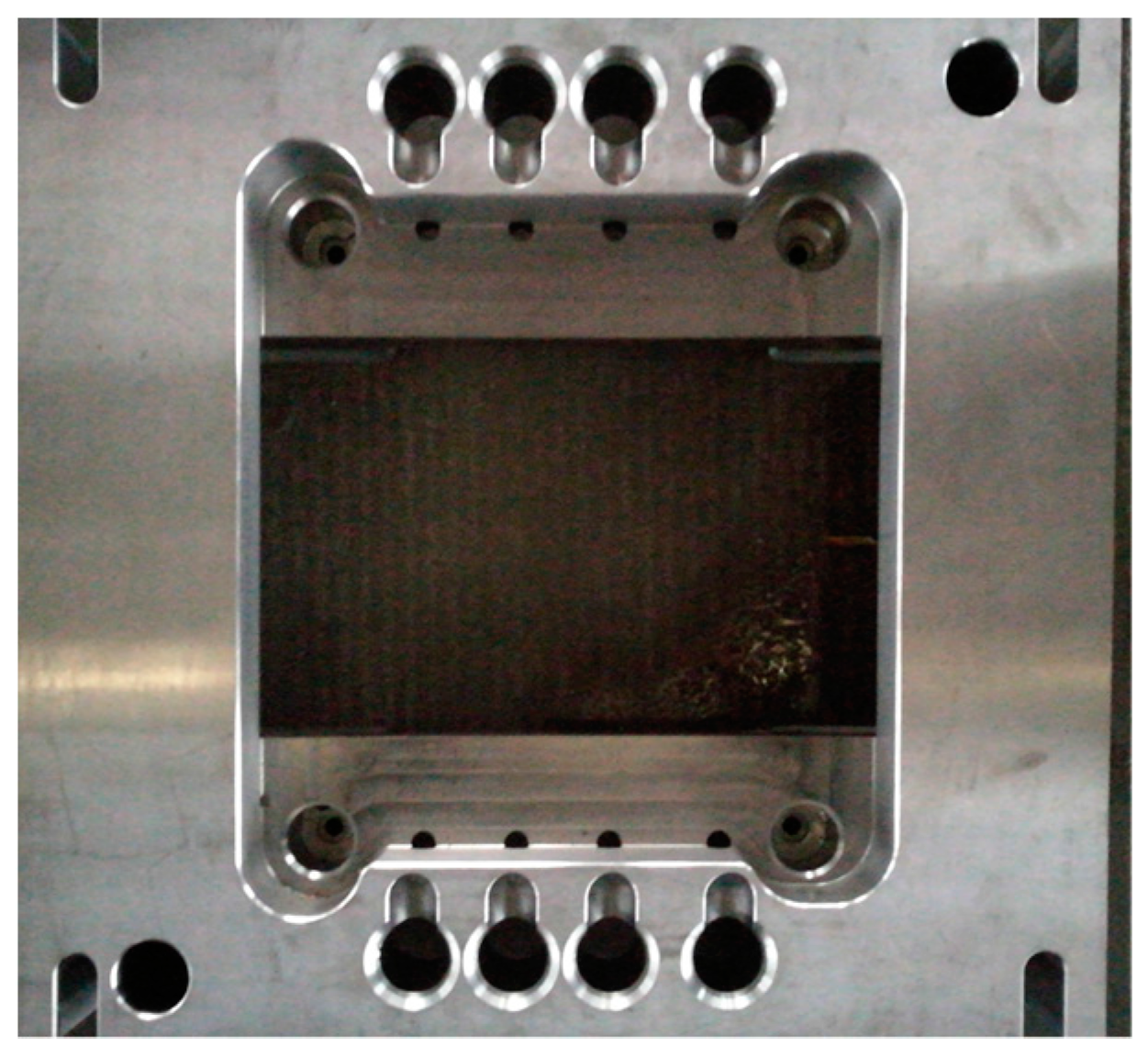
4.1. A Real Case Study
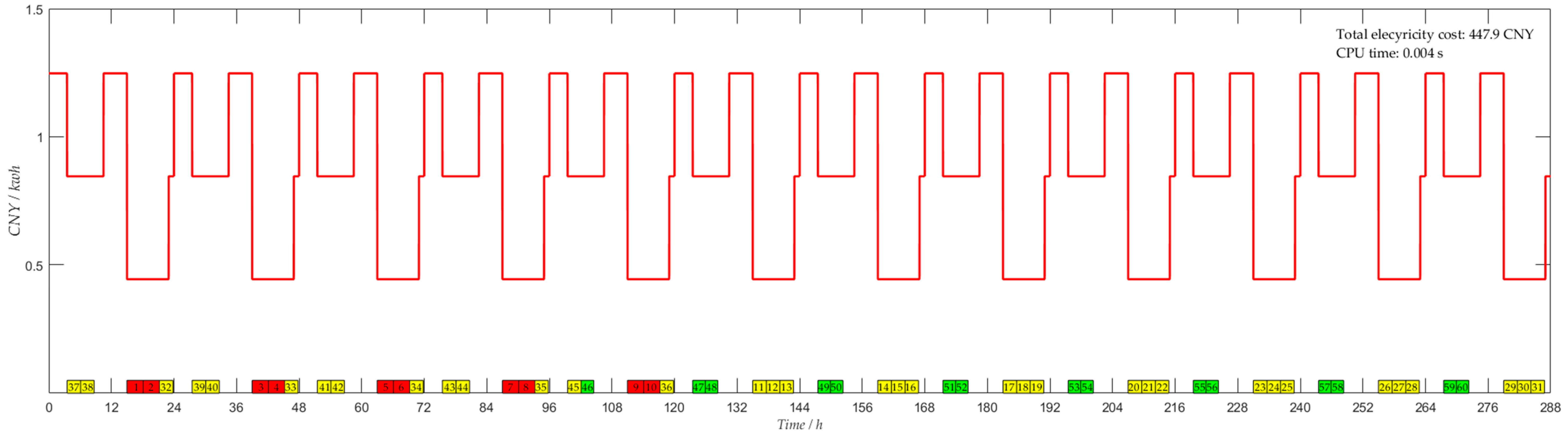
4.2. Randomly Generated Instances Studies
5. Conclusions and Prospects
Acknowledgments
Author Contributions
Conflicts of Interest
References
- International Energy Agency. World Energy Investment Outlook; International Energy Agency (IEA): Paris, France, 2015. [Google Scholar]
- Li, C.; Tang, Y.; Cui, L.; Li, P. A quantitative approach to analyze carbon emissions of CNC-based machining systems. J. Intell. Manuf. 2015, 26, 911–922. [Google Scholar] [CrossRef]
- Jovane, F.; Yoshikawa, H.; Alting, L.; Boër, C.R.; Westkamper, E.; Williams, D.; Tseng, M.; Seliger, G.; Paci, A.M. The incoming global technological and industrial revolution towards competitive sustainable manufacturing. CIRP Ann. Manuf. Technol. 2008, 57, 641–659. [Google Scholar] [CrossRef]
- Lu, C.; Gao, L.; Li, X.; Pan, Q.; Wang, Q. Energy-efficient permutation flow shop scheduling problem using a hybrid multi-objective backtracking search algorithm. J. Clean. Prod. 2017, 144, 228–238. [Google Scholar] [CrossRef]
- Sun, Z.; Li, L. Opportunity estimation for real-time energy control of sustainable manufacturing systems. IEEE Trans. Autom. Sci. Eng. 2013, 10, 38–44. [Google Scholar] [CrossRef]
- Park, C.W.; Kwon, K.S.; Kim, W.B.; Min, B.K.; Park, S.J.; Sung, I.H.; Yoon, Y.S.; Lee, K.S.; Lee, J.H.; Seok, J. Energy consumption reduction technology in manufacturing—A selective review of policies, standards, and research. Int. J. Precis. Eng. Manuf. 2009, 10, 151–173. [Google Scholar] [CrossRef]
- Ding, J.Y.; Song, S.; Zhang, R.; Chiong, R.; Wu, C. Parallel machine scheduling under time-of-use electricity prices: New models and optimization approaches. IEEE Trans. Autom. Sci. Eng. 2016, 13, 1138–1154. [Google Scholar] [CrossRef]
- Merkert, L.; Harjunkoski, I.; Isaksson, A.; Säynevirta, S.; Saarela, A.; Sand, G. Scheduling and energy—Industrial challenges and opportunities. Comput. Chem. Eng. 2015, 72, 183–198. [Google Scholar] [CrossRef]
- Che, A.; Zeng, Y.; Ke, L. An efficient greedy insertion heuristic for energy-conscious single machine scheduling problem under time-of-use electricity tariffs. J. Clean. Prod. 2016, 129, 565–577. [Google Scholar] [CrossRef]
- Longe, O.; Ouahada, K.; Rimer, S.; Harutyunyan, A.; Ferreira, H. Distributed demand side management with battery storage for smart home energy scheduling. Sustainability 2017, 9, 120. [Google Scholar] [CrossRef]
- Shapiro, S.A.; Tomain, J.P. Rethinking reform of electricity markets. Wake For. Law Rev. 2005, 40, 497–543. [Google Scholar]
- Zhang, H.; Zhao, F.; Fang, K.; Sutherland, J.W. Energy-conscious flow shop scheduling under time-of-use electricity tariffs. CIRP Ann. Manuf. Technol. 2014, 63, 37–40. [Google Scholar] [CrossRef]
- Che, A.; Wu, X.; Peng, J.; Yan, P. Energy-efficient bi-objective single-machine scheduling with power-down mechanism. Comput. Oper. Res. 2017, 85, 172–183. [Google Scholar] [CrossRef]
- He, F.; Shen, K.; Guan, L.; Jiang, M. Research on energy-saving scheduling of a forging stock charging furnace based on an improved SPEA2 algorithm. Sustainability 2017, 9, 2154. [Google Scholar] [CrossRef]
- Pruhs, K.; Stee, R.V.; Uthaisombut, P. Speed scaling of tasks with precedence constraints. In Proceedings of the 3rd International Workshop on Approximation and Online Algorithms, Palma de Mallorca, Spain, 6–7 October 2005; Erlebach, T., Persiano, G., Eds.; Springer: Berlin, Germany, 2005; pp. 307–319. [Google Scholar]
- Fang, K.; Uhan, N.; Zhao, F.; Sutherland, J.W. A new approach to scheduling in manufacturing for power consumption and carbon footprint reduction. J. Manuf. Syst. 2011, 30, 234–240. [Google Scholar] [CrossRef]
- Dai, M.; Tang, D.; Giret, A.; Salido, M.A.; Li, W.D. Energy-efficient scheduling for a flexible flow shop using an improved genetic-simulated annealing algorithm. Robot. Comput. Integr. Manuf. 2013, 29, 418–429. [Google Scholar] [CrossRef]
- Liu, C.H.; Huang, D.H. Reduction of power consumption and carbon footprints by applying multi-objective optimisation via genetic algorithms. Int. J. Prod. Res. 2014, 52, 337–352. [Google Scholar] [CrossRef]
- Mouzon, G.; Yildirim, M.B.; Twomey, J. Operational methods for minimization of energy consumption of manufacturing equipment. Int. J. Prod. Res. 2007, 45, 4247–4271. [Google Scholar] [CrossRef]
- Mouzon, G.; Yildirim, M. A framework to minimise total energy consumption and total tardiness on a single machine. Int. J. Sustain. Eng. 2008, 1, 105–116. [Google Scholar] [CrossRef]
- Liu, C.; Yang, J.; Lian, J.; Li, W.; Evans, S.; Yin, Y. Sustainable performance oriented operational decision-making of single machine systems with deterministic product arrival time. J. Clean. Prod. 2014, 85, 318–330. [Google Scholar] [CrossRef]
- Luo, H.; Du, B.; Huang, G.Q.; Chen, H.; Li, X. Hybrid flow shop scheduling considering machine electricity consumption cost. Int. J. Prod. Econ. 2013, 146, 423–439. [Google Scholar] [CrossRef]
- Sharma, A.; Zhao, F.; Sutherland, J.W. Econological scheduling of a manufacturing enterprise operating under a time-of-use electricity tariff. J. Clean. Prod. 2015, 108, 256–270. [Google Scholar] [CrossRef]
- Moon, J.-Y.; Shin, K.; Park, J. Optimization of production scheduling with time-dependent and machine-dependent electricity cost for industrial energy efficiency. Int. J. Adv. Manuf. Technol. 2013, 68, 523–535. [Google Scholar] [CrossRef]
- Che, A.; Zhang, S.; Wu, X. Energy-conscious unrelated parallel machine scheduling under time-of-use electricity tariffs. J. Clean. Prod. 2017, 156, 688–697. [Google Scholar] [CrossRef]
- Wang, S.; Liu, M.; Chu, F.; Chu, C. Bi-objective optimization of a single machine batch scheduling problem with energy cost consideration. J. Clean. Prod. 2016, 137, 1205–1215. [Google Scholar] [CrossRef]
- Shrouf, F.; Ordieres-Meré, J.; García-Sánchez, A.; Ortega-Mier, M. Optimizing the production scheduling of a single machine to minimize total energy consumption costs. J. Clean. Prod. 2014, 67, 197–207. [Google Scholar] [CrossRef]
- Gong, X.; Pessemier, T.D.; Joseph, W.; Martens, L. An energy-cost-aware scheduling methodology for sustainable manufacturing. In Proceedings of the 22nd CIRP Conference on Life Cycle Engineering (LCE) Univ New S Wales, Sydney, Australia, 7–9 April 2015; Kara, S., Ed.; Elsevier: Amsterdam, The Netherlands, 2015; pp. 185–190. [Google Scholar]
- Fang, K.; Uhan, N.A.; Zhao, F.; Sutherland, J.W. Scheduling on a single machine under time-of-use electricity tariffs. Ann. Oper. Res. 2016, 238, 199–227. [Google Scholar] [CrossRef]


| Period Type | Electricity Price (CNY/kwh) | Time Periods |
|---|---|---|
| On-peak | 1.2473 | 8:00–11:30 |
| 18:30–23:00 | ||
| Mid-peak | 0.8451 | 7:00–8:00 |
| 11:30–18:30 | ||
| Off-peak | 0.4430 | 23:00–7:00 |
| Product Model | Average Power Consumption Rate (kW) | Processing Time (h) | The Number of Parts |
|---|---|---|---|
| 40 | 4.4 | 2.4 | 15 |
| 70 | 4.7 | 2.6 | 35 |
| 100 | 5.3 | 3.1 | 10 |
| Part (Job) | 1 | 2 | 3 | 4 | 5 | 6 | 7 | 8 | 9 | 10 | 11 | 12 |
|---|---|---|---|---|---|---|---|---|---|---|---|---|
| Processing time (h) | 2.4 | 2.4 | 2.4 | 2.4 | 2.6 | 2.6 | 3.1 | 3.1 | 3.1 | 3.1 | 3.1 | 3.1 |
| Power consumption rate (kW) | 4.4 | 4.4 | 4.4 | 4.4 | 4.7 | 4.7 | 5.3 | 5.3 | 5.3 | 5.3 | 5.3 | 5.3 |
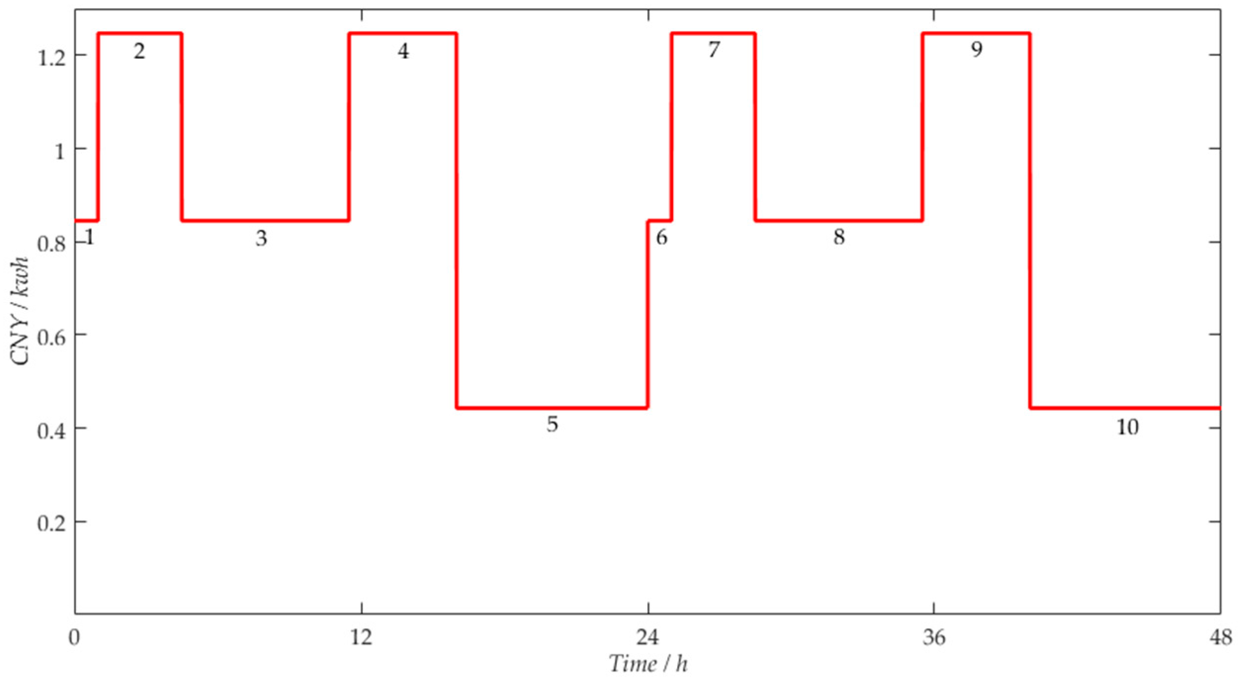
| Period | 1 | 2 | 3 | 4 | 5 | 6 | 7 | 8 | 9 | 10 |
|---|---|---|---|---|---|---|---|---|---|---|
| Duration (h) | 3.5 | 7 | 4.5 | 8 | 1 | 3.5 | 7 | 4.5 | 8 | 1 |
| Price (CNY/kwh) | 1.2473 | 0.8451 | 1.2473 | 0.443 | 0.8451 | 1.2473 | 0.8451 | 1.2473 | 0.443 | 0.8451 |
| Instance | GIH | GIH-F | ||||||
|---|---|---|---|---|---|---|---|---|
| n | e | m | TECH | CTH (s) | TECF | CTF (s) | G (%) | R |
| 20 | 1.2 | 12.0 | 1634.1 | 0.034 | 1632.5 | 0.002 | −0.10% | 17.0 |
| 1.5 | 15.0 | 1370.1 | 0.037 | 1370.1 | 0.002 | 0.00% | 18.5 | |
| 2.0 | 19.0 | 1295.7 | 0.041 | 1295.1 | 0.002 | −0.05% | 20.5 | |
| 3.0 | 28.5 | 1168.0 | 0.056 | 1168.0 | 0.001 | 0.00% | 56.0 | |
| 30 | 1.2 | 18.0 | 2414.6 | 0.064 | 2415.7 | 0.002 | 0.05% | 32.0 |
| 1.5 | 20.0 | 2274.6 | 0.065 | 2274.1 | 0.002 | −0.02% | 32.5 | |
| 2.0 | 28.5 | 2005.0 | 0.083 | 2005.0 | 0.002 | 0.00% | 41.5 | |
| 3.0 | 39.5 | 1741.0 | 0.119 | 1741.0 | 0.002 | 0.00% | 59.5 | |
| 40 | 1.2 | 23.0 | 3342.1 | 0.096 | 3342.0 | 0.004 | 0.00% | 24.0 |
| 1.5 | 28.0 | 2900.1 | 0.109 | 2899.3 | 0.003 | −0.03% | 36.3 | |
| 2.0 | 36.0 | 2775.6 | 0.143 | 2775.0 | 0.003 | −0.02% | 47.7 | |
| 3.0 | 52.0 | 2380.3 | 0.194 | 2380.3 | 0.002 | 0.00% | 97.0 | |
| 50 | 1.2 | 27.5 | 4242.5 | 0.137 | 4242.4 | 0.005 | 0.00% | 27.4 |
| 1.5 | 34.0 | 3733.0 | 0.164 | 3732.6 | 0.003 | −0.01% | 54.7 | |
| 2.0 | 43.0 | 3243.8 | 0.212 | 3243.2 | 0.004 | −0.02% | 53.0 | |
| 3.0 | 64.5 | 2940.6 | 0.315 | 2940.6 | 0.003 | 0.00% | 105.0 | |
| 60 | 1.2 | 34.0 | 4820.8 | 0.204 | 4819.7 | 0.006 | −0.02% | 34.0 |
| 1.5 | 40.0 | 4536.5 | 0.224 | 4536.3 | 0.004 | 0.00% | 56.0 | |
| 2.0 | 52.0 | 4029.0 | 0.293 | 4028.9 | 0.004 | 0.00% | 73.3 | |
| 3.0 | 78.0 | 3544.1 | 0.464 | 3544.1 | 0.004 | 0.00% | 116.0 | |
| 70 | 1.2 | 37.5 | 6133.5 | 0.249 | 6132.2 | 0.007 | −0.02% | 35.6 |
| 1.5 | 46.0 | 5416.3 | 0.303 | 5416.2 | 0.007 | 0.00% | 43.3 | |
| 2.0 | 61.0 | 4676.0 | 0.413 | 4675.8 | 0.004 | 0.00% | 103.3 | |
| 3.0 | 90.0 | 4024.9 | 0.643 | 4024.9 | 0.005 | 0.00% | 128.6 | |
| 80 | 1.2 | 43.0 | 7073.1 | 0.321 | 7072.9 | 0.009 | 0.00% | 35.7 |
| 1.5 | 53.0 | 6049.6 | 0.401 | 6049.6 | 0.006 | 0.00% | 66.8 | |
| 2.0 | 68.5 | 5348.1 | 0.554 | 5348.1 | 0.007 | 0.00% | 79.1 | |
| 3.0 | 101.5 | 4514.4 | 0.868 | 4514.3 | 0.005 | 0.00% | 173.6 | |
| 90 | 1.2 | 48.0 | 8128.5 | 0.399 | 8128.4 | 0.009 | 0.00% | 44.3 |
| 1.5 | 58.0 | 6772.5 | 0.501 | 6772.4 | 0.011 | 0.00% | 45.5 | |
| 2.0 | 77.5 | 6172.7 | 0.697 | 6172.6 | 0.008 | 0.00% | 87.1 | |
| 3.0 | 104.1 | 5228.2 | 1.196 | 5228.2 | 0.009 | 0.00% | 132.9 | |
| 100 | 1.2 | 53.5 | 8623.5 | 0.509 | 8622.9 | 0.017 | −0.01% | 29.9 |
| 1.5 | 64.0 | 7607.1 | 0.614 | 7607.0 | 0.011 | 0.00% | 55.8 | |
| 2.0 | 86.5 | 6896.8 | 0.927 | 6896.8 | 0.014 | 0.00% | 66.2 | |
| 3.0 | 128.0 | 5815.2 | 1.482 | 5815.1 | 0.009 | 0.00% | 164.7 | |
| Instance | GIH2 | GIH-F | |||||
|---|---|---|---|---|---|---|---|
| n | e | m | TECH | CTH2 (s) | TECF | CTF (s) | R |
| 500 | 1.2 | 250.5 | 43,909.1 | 53.0 | 43,909.1 | 0.219 | 242.0 |
| 1.5 | 315.0 | 38,637.8 | 52.2 | 38,637.9 | 0.187 | 279.1 | |
| 2.0 | 417.0 | 34,417.5 | 56.3 | 34,417.5 | 0.082 | 686.6 | |
| 3.0 | 628.5 | 28,948.1 | 56.9 | 28,948.0 | 0.093 | 611.8 | |
| 1000 | 1.2 | 504.0 | 87,500.3 | 244.2 | 87,500.3 | 1.802 | 135.5 |
| 1.5 | 628.5 | 77,598.3 | 230.3 | 77,597.0 | 0.873 | 263.8 | |
| 2.0 | 840.0 | 69,199.2 | 294.1 | 69,199.2 | 0.432 | 680.8 | |
| 3.0 | 1256.5 | 57,923.1 | 250.7 | 57,923.1 | 0.485 | 516.9 | |
| 2000 | 1.2 | 1002.5 | 176,681.2 | 3910.8 | 176,680.7 | 15.701 | 249.1 |
| 1.5 | 1255.5 | 155,205.3 | 3114.3 | 155,206.2 | 6.503 | 478.9 | |
| 2.0 | 1669.0 | 137,774.1 | 4316.2 | 137,774.1 | 3.346 | 1290.0 | |
| 3.0 | 2501.7 | 115,661.0 | 1785.8 | 115,661.0 | 3.574 | 499.7 | |
| 3000 | 1.2 | 1511.7 | 263,511.1 | 19,136.9 | 263,511.6 | 46.551 | 411.1 |
| 1.5 | 1880.0 | 231,954.6 | 14,429.7 | 231,954.9 | 25.560 | 564.5 | |
| 2.0 | 2483.3 | 205,368.8 | 19,759.8 | 205,368.8 | 11.219 | 1761.3 | |
| 3.0 | 3780.0 | 173,630.6 | 6571.9 | 173,630.6 | 12.432 | 528.6 | |
| 4000 | 1.2 | 1991.7 | 352,975.8 | 59,016.2 | 352,977.0 | 107.610 | 548.4 |
| 1.5 | 2511.7 | 306,983.3 | 43,971.5 | 306,983.3 | 66.669 | 659.5 | |
| 2.0 | 3335.0 | 275,694.8 | 60,539.8 | 275,694.8 | 26.281 | 2303.6 | |
| 3.0 | 4986.7 | 231,148.4 | 17,014.0 | 231,148.4 | 29.728 | 572.3 | |
| 5000 | 1.2 | 2498.3 | 438,717.9 | 136,314.9 | 438,718.6 | 168.581 | 808.6 |
| 1.5 | 3131.1 | 386,546.1 | 101,071.7 | 386,548.1 | 106.764 | 946.7 | |
| 2.0 | 4161.1 | 341,504.3 | 139,122.7 | 341,504.3 | 50.931 | 2731.6 | |
| 3.0 | 6257.8 | 291,685.7 | 51,471.0 | 291,685.7 | 58.821 | 875.0 | |
© 2018 by the authors. Licensee MDPI, Basel, Switzerland. This article is an open access article distributed under the terms and conditions of the Creative Commons Attribution (CC BY) license (http://creativecommons.org/licenses/by/4.0/).
Share and Cite
Zhang, H.; Fang, Y.; Pan, R.; Ge, C. A New Greedy Insertion Heuristic Algorithm with a Multi-Stage Filtering Mechanism for Energy-Efficient Single Machine Scheduling Problems. Algorithms 2018, 11, 18. https://doi.org/10.3390/a11020018
Zhang H, Fang Y, Pan R, Ge C. A New Greedy Insertion Heuristic Algorithm with a Multi-Stage Filtering Mechanism for Energy-Efficient Single Machine Scheduling Problems. Algorithms. 2018; 11(2):18. https://doi.org/10.3390/a11020018
Chicago/Turabian StyleZhang, Hongliang, Youcai Fang, Ruilin Pan, and Chuanming Ge. 2018. "A New Greedy Insertion Heuristic Algorithm with a Multi-Stage Filtering Mechanism for Energy-Efficient Single Machine Scheduling Problems" Algorithms 11, no. 2: 18. https://doi.org/10.3390/a11020018