Entropy-Based Algorithm for Supply-Chain Complexity Assessment

Abstract

This paper considers a graph model of hierarchical supply chains. The goal is to measure the complexity of links between different components of the chain, for instance, between the principal equipment manufacturer (a root node) and its suppliers (preceding supply nodes). The information entropy is used to serve as a measure of knowledge about the complexity of shortages and pitfalls in relationship between the supply chain components under uncertainty. The concept of conditional (relative) entropy is introduced which is a generalization of the conventional (non-relative) entropy. An entropy-based algorithm providing efficient assessment of the supply chain complexity as a function of the SC size is developed.

1. Introduction

This paper presents the entropy-based optimization model for estimating structural complexity of supply chain (SC), and, in particular, complexity of relationship between the principal equipment manufacturer (a root node) and its suppliers (preceding supply nodes). The information entropy is used as a measure of decision maker’s knowledge about the risks of shortages and pitfalls in relations between the supply chain components under uncertainty, the main attention being paid to relationships between the principal equipment manufacturer (a root node of the corresponding graph model) and its suppliers. A concept of the conditional (relative) entropy is introduced which is a generalization of the conventional (non-relative) entropy that provides more precise estimation of complexity in supply chains as it takes into account information flows between the components of different layers. A main advantage of the suggested entropy-based approach is that it can essentially simplify the hierarchical tree-like model of the supply chain, at the same time retaining the basic knowledge about main sources of risks in inter-layer relationships.

Processes of production, storage, transportation, and utilization of products in SCs may lead to many negative effects on the environment, such as emissions of pollutants into the air and soil; discharges of pollutants into surface and groundwater basins; pollution of soil and water with waste products of production, all these phenomena in their entirety deteriorating the relationships between manufacturing components and their suppliers. These and many other risky situations for manufacturing lead to the uncertainty in SC’s phases, i.e., engineering, procurement, production, and distribution [1]. The entropic approach developed in this paper aims at defining the best (minimal but sufficient) level of information going through the several supply chain phases. This paper analyzes the structural complexity of the supply chain affected by technological, organizational and environmental adverse events in the SCs, consequences of which lead, as a result, to violations of correct functioning of the SC. The detailed definition and analysis of the supply-chain structural complexity can be found in [2,3,4,5,6,7,8,9,10].

Similar to many other researchers (see, e.g., [11,12,13]), in order to accurately measure the risks of pitfalls and cases of failed supplies, this paper tends to determine the probabilities of undesirable events and their negative impacts on material, financial, and information flows. The economic losses are caused by failures to supply, shipments of inappropriate products, incomplete deliveries, delays in deliveries, etc., and the harmful effect of the adverse events may be expressed in monetary form by relevant penalties.

The main differences of the present work in comparison with close earlier papers (see, e.g., [7,12,14,15]) also exploiting the entropy approach for the SC complexity analysis are the following:

• This paper develops a new graph-theoretic model as a tool for selecting the most vulnerable disruption risks inside the SC which, in turn, can essentially decrease the size of the initial SC model without sacrificing essential knowledge about the risks;
• This paper introduces the conditional entropy as a tool for integrated analysis of the SC complexity under uncertainty, provides more precise estimation of the supply chain complexity taking into account links between the nodes of different layers;
• This paper suggests a new fast entropy-based algorithm for minimizing the SC size.

This paper is structured as follows. The related definitions from graph theory are presented in the next section. The definition of information entropy and the detailed problem description are given in Section 3. Section 4 describes the entropy-based algorithm permitting to reduce the SC model size without a loss of essential information. Section 5 describes the numerical example. Section 6 concludes the paper.

2. Basic Definitions

Wishing to avoid any ambiguity in further discussions, we begin with key definitions of risk and ambiguity in relationships between the manufacturer and its supplier. There is a wide specter of different definitions of risk and uncertainty. In this study, we follow Knight’s [16] view and his numerous followers. The uncertainty is the absence of certainty in our knowledge, or, in other words, a situation wherein it is impossible to precisely describe future outcomes. In the Knightian sense, the risk is measurable uncertainty, which is possible to calculate.

Similar to many other risk evaluators, we assume that the notion of risk can be described as the expected value of an undesirable outcome, that is, the product of two characteristics, the probability of an undesirable event (that is, a negative deviation of the delayed supply or failure to reach the planned supply target), and the impact or severity, that is, an expected loss in the case of the disruption affecting the supply of products across organizations in a supply network. In a situation with several possible accidents, we admit that the total risk is the sum of the risks for different accidents (see, e.g., [11,17,18]).

In the model considered below, an “event” is the observable discrete change in the state of the SC or its components. A “risk driver” is a factor, a driving force that may be a cause of the undesirable unforeseen event, such as disruptions, breakdowns, defects, mistakes in the design and planning, shortages of material in supply in the SC, etc. In this paper, we study the situations with an “observable uncertainty” where there is an objective opportunity to register, for a pre-specified period of time, the adverse events in the relationships between the components in the SC. Such a registration list, called a “risk protocol”, provides us the information whether or not the events are undesirable and, in the case if the event is undesirable what are its risk drivers and possible loss (see [12,19]). Such statistics in the risk protocols permits the decision maker to quantitatively evaluate a contribution of each driver and the total (entropy-based) observable information in the SC.

There exists a wide diversity of risk types, risk drivers, and options for their mitigation in the SC. Their taxonomy lies beyond the scope of this paper. Many authors noticed that if a researcher tries to analyze potential failures/disruptions of all the suppliers in a SC or their absolute majority, he/she encounters a simply impractical and unrealistic problem demanding an astronomic amount of time and budget. Moreover, the supply chain control of the root node of the supply chain is much more important than the control of any of its successors ([6,8]).

Consider a tree-type graph representing the hierarchical structure of an industrial supply chain Define the “parent layer”, called also the “main layer”, as consisting of a single node, as follows: L₀ = {n₀} where n₀ is the single node of the parent layer. Called also the original equipment manufacturer (OEM), or the root node. OEM is a firm (or company) that creates an end product, for, instance, assembles and creates an automobile.

Define a layer $L_s$ (also denoted as layer s) as the set of nodes which are on the same distance s from the root node n₀ in the underlying graph of the SC.

Layer 1 (also called Tier 1) are the companies supplying components directly to the OEM that set up the chain. In a typical supply chain, companies in Tier 2 supply the companies in Tier 1; Tier 3 supplies Tier 2, and so on. Tiered supply chains are common in industries such as aerospace or automotive manufacturing where the final product consists of many complex components and sub-assemblies.

Define a “cut” (also called a “cross-section”) $C_s$ as a union of all the layers $L_0,L_1,L_2,\dots L_s$, from 0 to s. It is evident that $C_0=L_0, C_{s-1}\subset C_s, C_s=\left\{C_{\left(s-1\right)},L_s\right\} s=1,2,\dots$, S.

Assume that, for each node of the SC, the list of risk drivers $F=\left\{f_1,f_2,\dots f_N\right\}$ is known, each being a source of different adverse events in the nodes of the SC. For simplicity, but without loss of generality, assume that any adverse event is caused by a single risk driver (otherwise, one can split such a multi-drive event into several elementary events each one being caused by a single driver). Here N is the total number of all the drivers.

Another basic assumption to be used in this work is that the drive factors are mutually dependent. It means, for example, that an unfavorable technological decision or an environmental pollution, that is, caused by a technology-based driver in some component at Tier 2 may lead to an adverse event in supply operations to a node at Tier 1. A technological mistake at Tier 3 may be a source of a delayed supply to Tier 2, and so on. In general, any factors f happening at tier s may be depending on a factor f′ at an earlier tier s + 1, f = 1,…, N; f′ = 1,…, N; s = 1,…, S. Below, the dependencies will be described with the help of the N × N matrix of relative probabilities.

The following Markovian property is assumed to take place. Assume that the dependence between any factor in tier s, on the one hand, and the factors in the lower tiers s + 1, s + 2,…, S actually exists only for the factors in a pair of neighboring tiers (s, s + 1), where s = 0,1,…, S. Moreover, assume that the pitfalls and any defective decisions do not flow downwards, that is, any risk factor in tier s does not depend upon the risk drivers in the nodes of higher layers, numbered s − 1, s − 2,…, 1.

In each layer s, when computing the probability of risk drivers f occurring in the nodes of the layer s, two types of adverse events have a place. First, there are the events (called “primary events” and denoted by A_f^prime(s)) that have happened in the nodes of layer s and which are caused by the risk driver f, f = 1,…, N. Second, there are the events (called “secondary events” and denoted by A_f^second(s + 1, s)) that have happened in the nodes of the next layer (s ± 1) but have an indirect impact upon inverse events in s, since the risk factors are dependent. More precisely, different drivers f′ in s+1 have impact upon the driver f in layer s, f = 1,…, N; f′ = 1,…, N; s = 1,2,…, S.

The impact from f′ to f is estimated with the help of the transition probability matrix M which is defined below and computed from the data in the risk protocols.

Denote by A_j(s) the following events:

A_f(s) = {risk driver f is the source of various adverse events in supply to all the nodes of layer s}, f = 1,…, N, s = 0,1,…, S.

Denote by p_f(s) = Pr (A_f(s)) the probability that the risk driver f is the source of different adverse events in supply in layer s,

$p_i\left(s\right)=\mathrm{Pr}\left(A_i\left(s\right)\right)$ = Pr {the risk driver f_i is the cause of adverse event on the layer s only}

Denote by p_f^prime(s) = Pr (A_f ^prime(s)) the probability that the risk driver f is the source of different adverse events in layer s, and which are caused by the risk driver f. These probabilities are termed as “primary”. Next, denote by p_f^second(s) = Pr (A_f ^second(s)) the probability that the risk driver f is a source of different adverse events in layer s which is a result of the indirect effect on the f by the risk drivers f′ that have caused the adverse events in layer s+1; these probabilities are termed as “secondary”.

Introduce the following notation:

$p_i^{\left(1\right)}\left(s\right)=\mathrm{Pr}\left(A_i^{prime}\left(s\right)\right)=\mathrm{Pr}\left(A_i^{\left(1\right)}\right)$ = Pr {the risk driver f_i is the cause of adverse event on the layer s only}

$p_i^{\left(2\right)}\left(s\right)=\mathrm{Pr}\left(A_i^{\sec ond}\left(s\right)\right)=\mathrm{Pr}\left(A_i^{\left(2\right)}\right)$ = Pr {the risk driver $f_i$ is the cause of adverse effect on the layer s as the result of the risk drivers on the layers s + 1}.

For simplicity, and without loss of generality, suppose that the list of risk drivers $F=\left\{f_1,f_2,\dots f_N\right\}$ is complete for each layer. Then the following holds

$${\displaystyle \sum _{i=1}^N{p}_i\left(s\right)}=1 \mathrm{for} s=0,1,2,\dots .$$

(1)

Denote $\overline{p}\left(s\right)=\left(p_1\left(s\right),p_2\left(s\right),\dots p_N\left(s\right)\right)$.

It is obvious that

$$A_i\left(s\right)=A_i^{\left(1\right)}\left(s\right)\cup A_i^{\left(2\right)}\left(s\right) \mathrm{and} A_i^{\left(1\right)}\left(s\right)\cap A_i^{\left(2\right)}\left(s\right)=\varnothing , j=1,2,\dots ,N.$$

Therefore,

$$p\left(A_i\left(s\right)\right)=p\left(A_i^{\left(1\right)}\left(s\right)\right)+p\left(A_i^{\left(2\right)}\left(s\right)\right)$$

or

$$p_i\left(s\right)=p_i^{\left(1\right)}\left(s\right)+p_i^{\left(2\right)}\left(s\right)\hspace{1em}i=1,2,\dots ,N.$$

(2)

Then the vector of risk driver probabilities $\overline{p}\left(s\right)=\left(p_1\left(s\right),p_2\left(s\right),\dots p_N\left(s\right)\right)$ can be decomposed into two vectors as

$$\overline{p}\left(s\right)={\overline{p}}^{\left(1\right)}\left(s\right)+{\overline{p}}^{\left(2\right)}\left(s\right),$$

(3)

where ${\overline{p}}^{\left(1\right)}\left(s\right)=\left(p_1^{\left(1\right)}\left(s\right),p_2^{\left(1\right)}\left(s\right),\dots ,p_N^{\left(1\right)}\left(s\right)\right)$ is the vector of drivers’ primary probabilities and ${\overline{p}}^{\left(2\right)}\left(s\right)=\left(p_1^{\left(2\right)}\left(s\right),p_2^{\left(2\right)}\left(s\right),\dots ,p_N^{\left(2\right)}\left(s\right)\right)$ the vector of drivers’ secondary probabilities.

For any layer s, define the transition matrix $M^{\left(2\right)}\left(s\right)$ of conditional probabilities of the risk drivers on layer s that are obtained as the result of risk drivers existing on layer s + 1

$$M^{\left(2\right)}\left(s\right)={\left(p_{ij}^{\left(2\right)}\left(s\right)\right)}_{N\times N}, s=0,1,2, \dots , \mathrm{with}$$

$$p_{ij}^{\left(2\right)}\left(s\right)=\mathrm{Pr}\left(A_j^{\left(2\right)}\left(s\right)|A_i\left(s+1\right)\right)i,\hspace{1em}j=1,2,\dots ,N,\hspace{1em}s=0,1,2\dots$$

(4)

Next, define the matrices $ML\left(s\right)$ of the primary drivers’ probabilities as

$$ML\left(s\right)={\left(q_{ij}\left(s\right)\right)}_{N\times N}, s=0,1,2, \dots ,$$

$$q_{ij}\left(s\right)=p_j^{\left(1\right)}\left(s\right),\hspace{1em}i,j=1,2,\dots ,N, s=0,1,\dots$$

$$ML\left(s\right)=\left(\begin{array}{ccccc}{p}_1^{\left(1\right)}\left(s\right)& p_2^{\left(1\right)}\left(s\right)& .& .& p_N^{\left(1\right)}\left(s\right)\\ p_1^{\left(1\right)}\left(s\right)& p_2^{\left(1\right)}\left(s\right)& .& .& p_N^{\left(1\right)}\left(s\right)\\ .& .& .& .& .\\ .& .& .& .& .\\ p_1^{\left(1\right)}\left(s\right)& p_2^{\left(1\right)}\left(s\right)& .& .& p_N^{\left(1\right)}\left(s\right)\end{array}\right)$$

(5)

Define the complete transition matrices as

$${\widehat{M}}^{\left(1\right)}\left(s\right)={\left({\widehat{p}}_{ij}^{\left(1\right)}\left(s\right)\right)}_{N\times N}, s=0,1,2, \dots , \mathrm{with}$$

$${\widehat{p}}_{ij}^{\left(1\right)}\left(s\right)=p_j^{\left(1\right)}\left(s\right)+p_{ij}^{\left(2\right)}\left(s\right), i,j=1,2,\dots ,N, s=0,1,2,\dots$$

(6)

From (5) and (6) it follows that

$${\widehat{M}}^{\left(1\right)}\left(s\right)=ML(s)+M^{\left(2\right)}\left(s\right), s=0,1,2\dots$$

(7)

$$p_j^{\left(2\right)}\left(A_j^{\left(2\right)}\left(s\right)\right)={\displaystyle \sum _{i=1}^N{p}_i\left(s+1\right)\cdot p_{ij}^{\left(2\right)}\left(s\right)},\hspace{1em}\hspace{1em}j=1,2,\dots ,N, s=0,1,\dots$$

or

$$p_j^{\left(2\right)}\left(A_j^{\left(2\right)}\left(s\right)\right)={\displaystyle \sum _{i=1}^N{p}_i\left(s+1\right)\cdot p_{ij}^{\left(2\right)}\left(s\right)},\hspace{1em}\hspace{1em}j=1,2,\dots ,N, s=0,1,\dots$$

(8)

In the matrix form, Equation (8) can be rewritten as

$${\overline{p}}^{\left(2\right)}\left(s\right)=\overline{p}\left(s+1\right)\cdot M^{\left(2\right)}\left(s\right),\hspace{1em}s=0,1,\dots$$

(9)

The following claim is true.

Claim.

The following relation holds:

$${\displaystyle \sum _{i=1}^N\left(p_i\left(s+1\right)\cdot \left({\displaystyle \sum _{j=1}^N{p}_{ij}^{\left(2\right)}\left(s\right)}\right)\right)}=1-{\displaystyle \sum _{j=1}^N{p}_j^{\left(1\right)}\left(s\right)}, s=0,1,\dots$$

(10)

The proof is straightforward and skipped here.

3. Information Entropy as a Measure of Supply Chain Complexity

Information entropy is defined by Shannon as follows [20]. Given a set of events E = {e₁,…, e_n} with a priori probabilities of event occurrence P = {p₁,…, p_n}, p_i ≥ 0, such that p_i + … + p_n = 1, the entropy function H is defined by

H = −∑_I p_i log p_i.

(11)

In order to yield all necessary information on the SC complexity issues, this paper uses the data recording of all adverse events occurred. The enterprise is to collect and store the data about main adverse events that occurred and led to economic losses in the enterprise, compensation cost, as well as the statistical analysis of the recorded data. Such requirement also applies to the registration of information about control of compliance of target and actual environmental characteristics.

Similar to [12], for each node u, consider an information database called a ‘risk protocol’. This is a registration list of most important events that have occurred in the node during a pre-specified time period. The protocol provides us the information whether or not the events are undesirable and, in the latter case, what are its risk drivers and possible losses.

This data is recorded in tables TBL_u, representing lists of events in each node u during a certain time period T (e.g., month, or year). Each row in the table corresponds to an individual event occurring in a given node at a certain time moment (for example, a day). We use symbol f as an index of risk drivers, F as the total number of risk drivers, and r as an index of the event (row). The value z_rf at the intersection of column f and row r is equal to 1 if the risk factor f is a source of the adverse event r, and 0—otherwise. The last column, F + 1, in each row (r) contains the magnitude of economic loss caused by the corresponding event r.

As far as the tables TBL_u, for all the nodes belonging to a certain arbitrary SC layer, says, are derived, all the tables are gathered into the Cut_Table CT_s for the entire SC cut. Let R_s(u) denote the total number of observed adverse (critical) events in a node u of cut C_s during a certain planning period. If such cut contains n(s) nodes, the total number of critical events in it is N^s = ∑_u=1,…,n(s) R_s(u). Assume that there are F risk drivers. For each risk driver f (f = 1, …, F), we can compute the number N_s(u, f) of critical events caused by driver f in the node u and the total number N_s(f) of critical events in all nodes of cut C_s, as registered in the risk protocols.

The relative frequency p_s(f) of that driver f is the source of different critical events in nodes of s and can be treated as the estimation of the corresponding probability. Then we compute the latter probability as

p_s(f) = N_s(f)/N^s

(12)

Then ∑_f p_s(f) = 1.

For the sake of simplicity of further analysis, our model applies to the case when the critical events are independent within the same tier and the losses are additive (these assumptions will be relaxed in our future research). For any node u from s, we can define corresponding probabilities p_s(u, f) of the event that a driver f is the source of adverse events in node u

p_s(u, f) = N_s(u, f)/R_s(u).

(13)

This paper treats the p_s(u, f) values defined by Equation(3) as probabilities of events participating in calculation of the entropy function in Equation (1).

The main idea of the suggested entropic approach is that the information entropy in this study estimates the average amount of information contained in a stream of critical events of the risk protocol. Thus the entropy characterizes our uncertainty, or the absence of knowledge, about the risks. The idea here is that the less the entropy is, the more information and knowledge about risks is available for the decision makers.

The entropy value can be computed iteratively for each cut of the SC. Assume that the nodes of a cut C_s−1, are defined at step (iteration) s − 1. Denote by T_s all supplier-nodes in the supply layer s of the given tree. Let L_s(T_s) denote the total losses defined by the risk protocol and summed up for all nodes of cut C_s in tiers T_s: L_s(T_s) = ∑_u∈Ts c_s(u). Further, let LT denote the total losses for all nodes of the entire chain. Thus, L_s(T_s) are contributions of the suppliers of cut C_s into the total losses LT.

Then L_s(T_s)/LT define the relative losses in the s-truncated supply chain. The relative contribution of lower tiers, that is, of those with larger s values, are, respectively, (LT − L_s(T_s))/LT. One can observe that the larger is the share (LT − L_s(T_s))/LT in comparison with L_s(T_s)/LT, the less is the available information about the losses in the cut C_s. For example, if the ratio L_s(T_s)/LT = 0.2, this case give us less information about the losses in cut C_s in comparison with the opposite case of L_s(T_s)/LT = 0.8. This argument motivates us to take the ratios (LT − L_s(T_s))/LT as the coefficients (weights) of the entropy (or, of our unawareness) about the economic losses incurred by adverse events affecting the environmental quality. In other words, the latter coefficients weigh the lack of our knowledge about the losses; as far as the number s grows, these coefficients become less and less significant.

Then the total entropy of all nodes u included into the cut s will be defined as

H(s) = ∑_u H(u)

(14)

where the weighted entropy in each node u is computed as

H(u) = −U_s ∑_f p_s(u, f) log p_s(u, f),

(15)

U_s = (LT − L_s(T_s))/LT,

(16)

Let x_u = 1 if node u from T_s is included into s, and x_u = 0, otherwise.

Then the total entropy of all nodes included into the cut s will be defined as

H(s) = ∑_u H(u) x_u,

(17)

where H(u) is defined in (15).

Computations of p_s(u, f) as well as the summation over risk factors f are taken in the risk event protocols for all the events related to nodes u from T_s. As far as entropy values are found for each node, the vulnerability to risks over the supply chain is measured as a total entropy of the s-truncated supply chain subject to the restricted losses.

Define the weighted entropy for each cut s as

$$H\left(C_s\right)=c\left(s\right)H^{*}\left(C_s\right)$$

(18)

where

$$H^{*}\left(C_s\right)=-{\displaystyle \sum _{j=1}^N{p}_j\left(C_s\right)\log p_j\left(C_s\right)}\text{ is the entropy of cut }{C}_s$$

We assume that the weight $c\left(s\right)$ satisfies the following conditions:

(i)

$c\left(s\right)$ is decreasing;

(ii)

$c\left(0\right)=L$;

(iii)

$\underset{s\to \infty }{{\displaystyle \lim }}c\left(s\right)=0$.

Define the “variation of relative entropy” depending upon the cut number is

$$REV\left(s\right)=\frac{H\left(s-1\right)-\frac{c\left(s-1\right)}{c\left(s\right)}H\left(s\right)}{H\left(1\right)-\frac{c\left(s-1\right)}{c\left(s\right)}H\left(s\right)}.$$

(19)

The following claim is valid:

Theorem.

For the process of sequentially computing of the relative entropy variation (REV), for any fixed value $\epsilon$, there exists the layer number s* for which it holds: $\left|REV\left(s*\right)\right|<\epsilon$.

Proof. 

For simplicity, we assume that the entropy of any layer depends only upon the information of the neighbor layers, that is,

$$H^{*}\left(L_s|L_{s+1},L_{s+2},\dots L_k\right)=H^{*}\left(L_s|L_{s+1}\right),\hspace{1em}\hspace{1em}s=0,1,2,\dots ,k-1$$

Let us exploit the following Formula for the entropy of combined system (see [21]):

$$H\left(X_1,X_2,\dots X_s\right)=H\left(X_1\right)+H\left(X_2|X_1\right)+H\left(X_3|X_1,X_2\right)+\dots +H\left(X_s|X_1,X_2,\dots ,X_{s-1}\right),$$

Applying it for the entropy $H^{*}\left(C_s\right)$ of cut $C_s$. We have

$$\begin{array}{l}{H}^{*}\left(C_s\right)=H^{*}\left(L_s,L_{s-1},L_{s-2},\dots ,L_0\right)=\\ =H^{*}(L_s)+H^{*}\left(L_{s-1}|L_s\right)+H^{*}\left(L_{s-2}|L_{s-1},L_s\right)+\dots +H^{*}\left(L_0|L_1,L_2,\dots L_s\right)=\\ =H^{*}(L_s)+H^{*}\left(L_{s-1}|L_s\right)+H^{*}\left(L_{s-2}|L_{s-1}\right)+\dots +H^{*}\left(L_0|L_1\right)\end{array}$$

(20)

Using the latter Formula for cut $C_{s-1}$, we obtain

$$H^{*}\left(C_{s-1}\right)=H^{*}(L_{s-1})+H^{*}\left(L_{s-2}|L_{s-1}\right)+H^{*}\left(L_{s-3}|L_{s-2}\right)+\dots +H^{*}\left(L_0|L_1\right)$$

(21)

From Formulas (20) and (21), we obtain that

$$H^{*}\left(C_s\right)=H^{*}\left(C_{s-1}\right)+H^{*}\left(L_s\right)-H^{*}\left(L_{s-1}\right)+H^{*}\left(L_{s-1}|L_s\right)$$

(22)

Here $H^{*}\left(L_{s-1}|L_s\right)$ denotes the conditional entropy of the layer s−1 under the condition that the probabilities and entropy of layer s are found.

Denote, for convenience, $H\left(C_s\right)=H\left(s\right)$ and $H^{*}\left(C_s\right)=H^{*}\left(s\right)$.

Using the definition of the weighted entropy and Formula (21), we obtain

$$H\left(s\right)=c\left(s\right)H^{*}\left(s\right)=c\left(s\right)\left(H^{*}\left(C_{s-1}\right)+H^{*}\left(L_s\right)-H^{*}\left(L_{s-1}\right)+H^{*}\left(L_{s-1}|L_s\right)\right).$$

Using the Formula of the conditional entropy, the definitions of events $A_i\left(s\right)$, probabilities $p_i\left(s\right)$ and matrices $M^{\left(2\right)}\left(s\right)$, we can write that

$$\begin{array}{l}{H}^{*}\left(L_{s-1}|L_s\right)=-{\displaystyle \sum _{i=1}^N\left(P\left(A_i\left(s\right)\right)\cdot {\displaystyle \sum _{j=1}^{N}P\left(A_j\left(s-1\right)|A_i\left(s\right)\right)\cdot \mathrm{logP}\left(A_j\left(s-1\right)|A_i\left(s\right)\right)}\right)}\\ =-{\displaystyle \sum _{i=1}^N\left(p_i\left(s\right)\cdot {\displaystyle \sum _{j=1}^N{\widehat{p}}_{ij}^{\left(1\right)}\left(s-1\right)\cdot \log \left({\widehat{p}}_{ij}^{\left(1\right)}\left(s-1\right)\right)}\right)}\end{array}$$

$$H^{*}\left(L_{s-1}|L_s\right)=-{\displaystyle \sum _{i=1}^N\left(p_i\left(s\right)\cdot {\displaystyle \sum _{j=1}^N{\widehat{p}}_{ij}^{\left(1\right)}\left(s-1\right)\cdot \log \left({\widehat{p}}^{\left(1\right)}\left(s-1\right)\right)}\right)}$$

(23)

Using Formula (22) we can write

$$H\left(s\right)=c\left(s\right)\left(H^{*}\left(C_{s-1}\right)+H^{*}\left(L_s\right)-H^{*}\left(L_{s-1}\right)-{\displaystyle \sum _{i=1}^N\left(p_i\left(s\right)\cdot {\displaystyle \sum _{j=1}^N{\widehat{p}}_{ij}^{\left(1\right)}\left(s-1\right)\cdot \log \left({\widehat{p}}_{ij}^{\left(1\right)}\left(s-1\right)\right)}\right)}\right)$$

(24)

$$s=1,2,\dots$$

$$\begin{array}{l}H\left(s-1\right)-H\left(s\right)=\\ =H\left(s-1\right)-c\left(s\right)\left(H^{*}\left(C_{s-1}\right)+H^{*}\left(L_s\right)-H^{*}\left(L_{s-1}\right)-{\displaystyle \sum _{i=1}^N\left(p_i\left(s\right)\cdot {\displaystyle \sum _{j=1}^N{\widehat{p}}_{ij}^{\left(1\right)}\left(s-1\right)\cdot \log \left({\widehat{p}}_{ij}^{\left(1\right)}\left(s-1\right)\right)}\right)}\right)=\\ =\left(1-\frac{c\left(s\right)}{c\left(s-1\right)}\right)H\left(s-1\right)-c\left(s\right)\left(H^{*}\left(L_s\right)-H^{*}\left(L_{s-1}\right)\right)+c\left(s\right){\displaystyle \sum _{i=1}^N\left(p_i\left(s\right)\cdot {\displaystyle \sum _{j=1}^N{\widehat{p}}_{ij}^{\left(1\right)}\left(s-1\right)\cdot \log \left({\widehat{p}}_{ij}^{\left(1\right)}\left(s-1\right)\right)}\right)}\end{array}.$$

We obtain that

$$H\left(s-1\right)-H\left(s\right)=\left(1-\frac{c\left(s\right)}{c\left(s-1\right)}\right)H\left(s-1\right)-c\left(s\right)\left(H^{*}\left(L_s\right)-H^{*}\left(L_{s-1}\right)\right)+c\left(s\right)\cdot {\displaystyle \sum _{i=1}^N\left(p_i\left(s\right)\cdot {\displaystyle \sum _{j=1}^N{\widehat{p}}_{ij}^{(1)}\left(s-1\right)\cdot \log \left({\widehat{p}}_{ij}^{(1)}\left(s-1\right)\right)}\right)}$$

(25)

$$s=1,2,\dots$$

Since the following relations are valid,

$$\begin{array}{l}0<1-\frac{c\left(s\right)}{c\left(s-1\right)}<1,\\ 0<-{\displaystyle \sum _{i=1}^N\left(p_i\left(s\right)\cdot {\displaystyle \sum _{j=1}^N{\widehat{p}}_{ij}^{\left(1\right)}\left(s-1\right)\cdot \log \left({\widehat{p}}_{ij}^{\left(1\right)}\left(s-1\right)\right)}\right)}<\log N\\ 0<H^{*}\left(L_s\right)<\log N,\hspace{1em}0<H^{*}\left(L_{s-1}\right)<\log N\\ \underset{s\to \infty }{{\displaystyle \lim }} H\left(s-1\right)=0,\hspace{1em} \underset{s\to \infty }{{\displaystyle \lim }} c\left(s\right)=0\end{array}$$

we obtain that

$$\underset{s\to \infty }{{\displaystyle \lim }}\left(H\left(s-1\right)-H\left(s\right)\right)=0$$

Therefore, for any accuracy level ε, we can select the number of a cut $s_1$ for which

$$\frac{H\left(s_1-1\right)-H\left(s_1\right)}{H\left(0\right)-H\left(s_1\right)}<\epsilon$$

The truncated part of the SC containing only layers of the cut $\left(s_1-1\right)$ possesses the required level of the entropy variation. The theorem is proved.

The theorem permits the decision maker to define the decreased size of the SC model, such that the decreased number of the layers in the SC model is sufficient for planning and coordinating the knowledge about the risks in the relations between the SC components, without the loss of essential information about the risks.

4. Entropy-Based Algorithm for Complexity Assessment

This section summarizes theoretical findings of the previous sections for obtaining a decreased SC model on which planning and coordination of supplies can be done without loss of essential information.

Input data of the algorithm:

• the given number N of risk drivers,
• weight functions $c\left(s\right)$ selected by the decision maker,
• probabilities p_f^prime(s) = Pr (A_f ^prime(s)) that the risk driver f is the direct source of the supply failure/delay in layer s, which are caused by risk driver f,
• probabilities p_f^second(s) = Pr (A_f ^second(s)) that the risk driver f is the source of the supply failure/delay in layer s, which is a result of the indirect effect on the f by the risk drivers f′ of supply delay in layer s + 1; these probabilities are termed as secondary.
• transition probability matrices $M^{\left(2\right)}\left(s\right)={\left(p_{ij}^{\left(2\right)}\left(s\right)\right)}_{N\times N}$, s = 0, 1,2,…, k.

Step 1. Using the entropy Formulas (11)–(17), calculate entropy of the layer 0:

$$\begin{array}{l}{H}^{*}\left(L_0\right)=-{\displaystyle \sum _{j=1}^N{p}_j\left(0\right)}\log \left(p_j\left(0\right)\right)\\ H\left(0\right)=H^{*}\left(L_0\right)\end{array}$$

Step 2. Using Formulas (2)–(9), compute the matrix

${\widehat{M}}^{\left(1\right)}\left(0\right)$, and vector $\overline{p}\left(1\right)=\left(p_1\left(1\right),p_2\left(1\right),\dots p_N\left(1\right)\right)$

Step 3. Compute the corrected vector of probabilities for the layer $L_0$, using Formula

${\overline{p}}^c\left(0\right)=\overline{p}\left(1\right)\cdot {\widehat{M}}^{\left(1\right)}\left(0\right)$ and corrected entropy for layer $L_0$

$$H{C}^{*}\left(L_0\right)=-{\displaystyle \sum _{j=1}^N{p}_j^c\left(0\right)}\log \left(p_j^c\left(0\right)\right)$$

Step 4. For s = 2,3,…, using matrix ${\widehat{M}}^{\left(1\right)}\left(s\right)$, vector $\overline{p}\left(s\right)=\left(p_1\left(s\right),p_2\left(s\right),\dots p_N\left(s\right)\right)$ compute sequentially the corrected vectors of probabilities for the layers $L_{s-1}$: ${\overline{p}}^c\left(s-1\right)=\overline{p}\left(s\right)\cdot {\widehat{M}}^{\left(1\right)}\left(s-1\right)$

Step 5. Compute $H{C}^{*}\left(L_{s-1}\right)=-{\displaystyle \sum _{j=1}^N{p}_j^c\left(s-1\right)}\log \left(p_j^c\left(s-1\right)\right)$

Step 6. Compute

$$\begin{array}{l}H\left(0\right)-H\left(1\right)=\\ =\left(1-\frac{c\left(1\right)}{c\left(0\right)}\right)H\left(0\right)-c\left(1\right)\left(H^{*}\left(L_1\right)-H{C}^{*}\left(L_0\right)\right)+c\left(1\right){\displaystyle \sum _{i=1}^N\left(p_i\left(1\right)\cdot {\displaystyle \sum _{j=1}^N{\widehat{p}}_{ij}^{\left(1\right)}\left(0\right)\cdot \log \left({\widehat{p}}_{ij}^{\left(1\right)}\left(0\right)\right)}\right)}\end{array}$$

Step 7. For s − 1,2,…, compute

$$\begin{array}{l}H\left(s-1\right)-H\left(s\right)=\\ =\left(1-\frac{c\left(s\right)}{c\left(s-1\right)}\right)H\left(s-1\right)-c\left(s\right)\left(H^{*}\left(L_s\right)-H{C}^{*}\left(L_{s-1}\right)\right)+c\left(s\right){\displaystyle \sum _{i=1}^N\left(p_i\left(s\right)\cdot {\displaystyle \sum _{j=1}^N{\widehat{p}}_{ij}^{\left(1\right)}\left(s-1\right)\cdot \log \left({\widehat{p}}_{ij}^{\left(1\right)}\left(s-1\right)\right)}\right)}\end{array}$$

As the stopping rule use the following rule:

Stop at the cut $s_1$ for which $\frac{H\left(s_1-1\right)-H\left(s_1\right)}{H\left(0\right)-H\left(s_1\right)}<\epsilon$ holds.

Then the reduced SC model contains only the cut $\left(s_1-1\right)$.

5. Numerical Example

Input data:

-

the number or risk factor drivers in each layer, N = 3;

-

level of accuracy $\epsilon =0.01$;

-

the weight function $c\left(s\right)=\frac{1}{{\left(s+1\right)}^2}$ (selected by the decision maker).

-

probabilities p_f^prime(s) = Pr (A_f ^prime(s))

$$\begin{array}{l}{\overline{p}}_{\mathrm{f}}{}^{\mathrm{prime}}\left(0\right)=\left(0.34570.08350.0918\right)\\ {\overline{p}}_{\mathrm{f}}{}^{\mathrm{prime}}\left(1\right)=\left(0.16440.30170.0542\right)\\ {\overline{p}}_{\mathrm{f}}{}^{\mathrm{prime}}\left(2\right)=\left(0.12560.16020.2156\right)\\ {\overline{p}}_{\mathrm{f}}{}^{\mathrm{prime}}\left(3\right)=\left(0.08450.20010.3025\right)\\ {\overline{p}}_{\mathrm{f}}{}^{\mathrm{prime}}\left(4\right)=\left(0.26230.10560.2369\right)\\ {\overline{p}}_{\mathrm{f}}{}^{\mathrm{prime}}\left(5\right)=\left(0.20140.20320.1356\right)\\ {\overline{p}}_{\mathrm{f}}{}^{\mathrm{prime}}\left(6\right)=\left(0.14220.22580.1047\right)\\ {\overline{p}}_{\mathrm{f}}{}^{\mathrm{prime}}\left(7\right)=\left(0.10560.32410.2658\right)\\ {\overline{p}}_{\mathrm{f}}{}^{\mathrm{prime}}\left(8\right)=\left(0.15990.30560.1422\right)\\ {\overline{p}}_{\mathrm{f}}{}^{\mathrm{prime}}\left(9\right)=\left(0.20140.30680.0856\right)\\ {\overline{p}}_{\mathrm{f}}{}^{\mathrm{prime}}\left(10\right)=\left(0.21450.02410.2536\right)\end{array}$$

-

probabilities p_f^second(s) = Pr (A_f ^second(s))

$$\begin{array}{l}{\overline{p}}_{\mathrm{f}}{}^{\mathrm{second}}\left(0\right)=\left(0.30140.07250.1051\right)\\ {\overline{p}}_{\mathrm{f}}{}^{\mathrm{second}}\left(1\right)=\left(0.18510.25320.0414\right)\\ {\overline{p}}_{\mathrm{f}}{}^{\mathrm{second}}\left(2\right)=\left(0.20980.13080.1280\right)\\ {\overline{p}}_{\mathrm{f}}{}^{\mathrm{second}}\left(3\right)=\left(0.08370.20110.1281\right)\\ {\overline{p}}_{\mathrm{f}}{}^{\mathrm{second}}\left(4\right)=\left(0.12720.10130.1667\right)\\ {\overline{p}}_{\mathrm{f}}{}^{\mathrm{second}}\left(5\right)=\left(0.23340.06870.1577\right)\\ {\overline{p}}_{\mathrm{f}}{}^{\mathrm{second}}\left(6\right)=\left(0.13930.27090.1171\right)\\ {\overline{p}}_{\mathrm{f}}{}^{\mathrm{second}}\left(7\right)=\left(0.08240.18030.0417\right)\\ {\overline{p}}_{\mathrm{f}}{}^{\mathrm{second}}\left(8\right)=\left(0.13790.11430.1401\right)\\ {\overline{p}}_{\mathrm{f}}{}^{\mathrm{second}}\left(9\right)=\left(0.14560.17030.0903\right)\\ {\overline{p}}_{\mathrm{f}}{}^{\mathrm{second}}\left(10\right)=\left(0.23500.03830.2345\right)\end{array}$$

transition probability matrices $M^{\left(2\right)}\left(s\right)={\left(p_{ij}^{\left(2\right)}\left(s\right)\right)}_{N\times N}$, s = 1,2,…,10,

$$\begin{array}{l}{M}^{\left(2\right)}\left(1\right)=\\ \\ 0.31240.33200.3556\\ 0.34560.41580.2386\\ 0.42580.02560.5486\end{array}$$

$$\begin{array}{l}{M}^{\left(2\right)}\left(2\right)=\\ \\ 0.25870.35680.3845\\ 0.65870.02540.3159\\ 0.48720.02460.4882\end{array}$$

$$\begin{array}{l}{M}^{\left(2\right)}\left(3\right)=\\ \\ 0.10540.45030.4443\\ 0.08650.65140.2621\\ 0.45360.14580.4006\\ \\ M^{\left(2\right)}\left(4\right)=\\ \\ 0.35480.21490.4303\\ 0.28260.52390.1935\\ 0.25960.68230.0581\end{array}$$

$$\begin{array}{l}{M}^{\left(2\right)}\left(5\right)=\\ \\ 0.10360.54830.3481\\ 0.05980.21360.7266\\ 0.12690.24560.6275\\ \\ M^{\left(2\right)}\left(6\right)=\\ \\ 0.32650.42510.2484\\ 0.64210.23860.1193\\ 0.04250.12430.8332\\ \\ M^{\left(2\right)}\left(7\right)=\\ \\ 0.09340.46520.4414\\ 0.52190.13610.3420\\ 0.45820.03480.5070\end{array}$$

$$\begin{array}{l}{M}^{\left(2\right)}\left(8\right)=\\ \\ 0.24580.19650.5577\\ 0.05630.75810.1856\\ 0.41030.17840.4113\\ \\ M^{\left(2\right)}\left(9\right)=\\ \\ 0.43970.15350.4068\\ 0.36270.48630.1510\\ 0.26420.55290.1829\\ \\ M^{\left(2\right)}\left(10\right)=\\ \\ 0.74120.09850.1603\\ 0.05250.43680.5107\\ 0.10560.72960.1648\end{array}$$

The algorithm solves this example as follows.

Using Formulas (3)–(6) compute:

The probabilities of risk factor drivers on the layers $L_0,L_1,L_2,\dots$

$$\begin{array}{l}\overline{p}\left(0\right)=\left(0.64710.15600.1969\right)\\ \overline{p}\left(1\right)=\left(0.34950.55490.0956\right)\\ \overline{p}\left(2\right)=\left(0.33540.29100.3736\right)\\ \overline{p}\left(3\right)=\left(0.16820.40120.4306\right)\\ \overline{p}\left(4\right)=\left(0.38950.20690.4036\right)\\ \overline{p}\left(5\right)=\left(0.43480.27190.2933\right)\\ \overline{p}\left(6\right)=\left(0.28150.49670.2218\right)\\ \overline{p}\left(7\right)=\left(0.18800.50440.3075\right)\\ \overline{p}\left(8\right)=\left(0.29780.41990.2823\right)\\ \overline{p}\left(9\right)=\left(0.34700.47710.1759\right)\\ \overline{p}\left(10\right)=\left(0.44950.06240.4881\right)\end{array}$$

The complete transition matrices

$${\widehat{M}}^{\left(1\right)}\left(s\right)={\left({\widehat{p}}_{ij}^{\left(1\right)}\left(s\right)\right)}_{3\times 3}$$

$$\begin{array}{l}\\ {\widehat{M}}^{\left(1\right)}\left(s\right)=\left(p_{ij}\left(s\right)\right),s=1,2,\dots ,10\\ \\ \widehat{M}(:,:,1)=\\ \\ 0.41240.42270.1649\\ 0.80760.01300.1794\\ 0.57320.01140.4153\end{array}$$

$$\begin{array}{l}\widehat{M}(:,:,2)=\\ \\ 0.19780.65670.1455\\ 0.10290.85990.0372\\ 0.67790.22580.0963\\ \\ \widehat{M}(:,:,3)=\\ \\ 0.63310.31760.0494\\ 0.14940.02750.8230\\ 0.39250.52610.0814\end{array}$$

$$\begin{array}{l}\\ \widehat{M}(:,:,4)=\\ \\ 0.11040.87430.0153\\ 0.12620.04550.8284\\ 0.24540.12700.6276\\ \\ \\ \widehat{M}(:,:,5)=\\ \\ 0.40190.30970.2884\\ 0.71730.24440.0382\\ 0.06720.01970.9131\\ \\ \widehat{M}(:,:,6)=\\ \\ 0.13990.62220.2379\\ 0.48870.16860.3427\\ 0.68850.05840.2531\end{array}$$

$$\begin{array}{l}\widehat{M}(:,:,7)=\\ \\ 0.51050.11900.3705\\ 0.33770.44720.2152\\ 0.04930.80890.1418\end{array}$$

$$\begin{array}{l}\widehat{M}(:,:,8)=\\ \\ 0.19300.22890.5781\\ 0.07010.88850.0414\\ 0.35810.22380.4180\\ \\ \widehat{M}(:,:,9)=\\ \\ 0.44870.22710.3242\\ 0.25540.43090.3137\\ 0.11510.77060.1143\\ \\ \widehat{M}(:,:,10)=\\ \\ 0.67510.12300.2019\\ 0.02870.33830.6330\\ 0.08560.82100.0934\end{array}$$

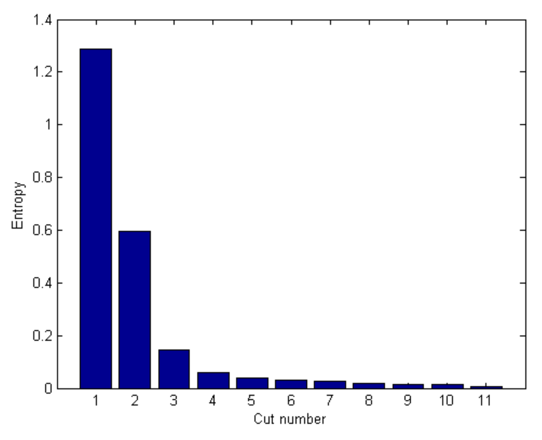
Omitting intermediate calculations, at Steps 6 and 7, the algorithm computes values H(s) and REV(s) for each cut s, as presented in

Table 1. Computational results.

S	0	1	2	3	4	5	6
H(s)	2.5693	1.2861	0.5972	0.1735	0.0953	0.0378	0.0235
REV(s)	-	1	0.5368	0.3301	0.0609	0.0448	0.0111

.

We observe that REV(6) value is less then $\epsilon =0.01$, therefore we can reduce our SC size by taking the truncated model with s = 6. The results of computations are graphically presented in Figure 1.

6. Conclusions

A main contribution of this paper is the entropy-based method for a quantitative assessment of the information and knowledge relevant to the analysis of the SC size and complexity. Using the entropy approach, the suggested model extracts a sufficient amount of useful information from the risk protocols generated at different SC units. Assessment of the level of entropy for the risks allows the decision maker, step by step, to assess the entropy in the SC model and, consequently, to increase the amount of useful knowledge. As a result, we arrive at a reduced graph model of the supply chain such that it contains essentially the same amount of information about controllable parameters as the complete SC graph but much smaller in size.

An attractive direction for further research is to incorporate the human factor and, in particular, the effect of human fatigue (see [22]) on performance of industrial supply chains under uncertainty in dynamic environments.

References

- Fera, M.; Fruggiero, F.; Lambiase, A.; Macchiaroli, R.; Miranda, S. The role of uncertainty in supply chains under dynamic modeling. Int. J. Ind. Eng. Comput. 2017, 8, 119–140. [Google Scholar] [CrossRef]
- Calinescu, A.; Efstathiou, J.; Schirn, J.; Bermejo, J. Applying and assessing two methods for measuring complexity in manufacturing. J. Oper. Res. Soc. 1998, 49, 723–733. [Google Scholar] [CrossRef]
- Sivadasan, S.; Efstathiou, J.; Calinescu, A.; Huatuco, L.H. Advances on measuring the operational complexity of supplier–customer systems. Eur. J. Oper. Res. 2006, 171, 208–226. [Google Scholar] [CrossRef]
- Sivadasan, S.; Efstathiou, J.; Frizelle, G.; Shirazi, R.; Calinescu, A. An information-theoretic methodology for measuring the operational complexity of supplier-customer systems. Int. J. Oper. Prod. Manag. 2002, 22, 80–102. [Google Scholar] [CrossRef]
- Sivadasan, S.; Smart, J.; Huatuco, L.H.; Calinescu, A. Reducing schedule instability by identifying and omitting complexity-adding information flows at the supplier–customer interface. Int. J. Prod. Econ. 2013, 145, 253–262. [Google Scholar] [CrossRef]
- Battini, D.; Persona, A. Towards a Use of Network Analysis: Quantifying the Complexity of Supply Chain Networks. Int. J. Electron. Cust. Relatsh. Manag. 2007, 1, 75–90. [Google Scholar] [CrossRef]
- Isik, F. An Entropy-based Approach for Measuring Complexity in Supply Chains. Int. J. Prod. Res. 2010, 48, 3681–3696. [Google Scholar] [CrossRef]
- Allesina, S.; Azzi, A.; Battini, D.; Regattieri, A. Performance Measurement in Supply Chains: New Network Analysis and Entropic Indexes. Int. J. Prod. Res. 2010, 48, 2297–2321. [Google Scholar] [CrossRef]
- Modraka, V.; Martona, D. Structural Complexity of Assembly Supply Chains: A Theoretical Framework. Proced. CIRP 2013, 7, 43–48. [Google Scholar] [CrossRef]
- Ivanov, D. Entropy-Based Supply Chain Structural Complexity Analysis. In Structural Dynamics and Resilience in Supply Chain Risk Management; International Series in Operations Research & Management Science; Springer: Berlin, Germany, 2018; Volume 265, pp. 275–292. [Google Scholar]
- Kogan, K.; Tapiero, C.S. Supply Chain Games: Operations Management and Risk Valuation; Springer: New York, NY, USA, 2007. [Google Scholar]
- Levner, E.; Ptuskin, A. An entropy-based approach to identifying vulnerable components in a supply chain. Int. J. Prod. Res. 2015, 53, 6888–6902. [Google Scholar] [CrossRef]
- Aven, T. Risk Analysis; Wiley: New York, NY, USA, 2015. [Google Scholar]
- Harremoës, P.; Topsøe, F. Maximum entropy fundamentals. Entropy 2001, 3, 191–226. [Google Scholar] [CrossRef]
- Herbon, A.; Levner, E.; Hovav, S.; Shaopei, L. Selection of Most Informative Components in Risk Mitigation Analysis of Supply Networks: An Information-gain Approach. Int. J. Innov. Manag. Technol. 2012, 3, 267–271. [Google Scholar]
- Knight, F.H. Risk, Uncertainty, and Profit; Hart, Schaffner & Marx: Boston, MA, USA, 1921. [Google Scholar]
- Zsidisin, G.A.; Ellram, L.M.; Carter, J.R.; Cavinato, J.L. An Analysis of Supply Risk Assessment Techniques. Int. J. Phys. Distrib. Logist. Manag. 2004, 34, 397–413. [Google Scholar] [CrossRef]
- Tapiero, C.S.; Kogan, K. Risk and Quality Control in a Supply Chain: Competitive and Collaborative Approaches. J. Oper. Res. Soc. 2007, 58, 1440–1448. [Google Scholar] [CrossRef]
- Tillman, P. An Analysis of the Effect of the Enterprise Risk Management Maturity on Sharehokder Value during the Economic Downturn of 2008–2010. Master’s Thesis, University of Pretoria, Pretoria, South Africa, 2011. [Google Scholar]
- Shannon, C.E. A Mathematical Theory of Communication. Bell Syst. Tech. J. 1948, 27, 379–423. [Google Scholar] [CrossRef]
- Wentzel, E.S. Probability Theory; Mir Publishers: Moscow, Russia, 1982. [Google Scholar]
- Fruggiero, F.; Riemma, S.; Ouazene, Y.; Macchiaroli, R.; Guglielmim, V. Incorporating the human factor within the manufacturing dynamics. IFAC-PapersOnline 2016, 49, 1691–1696. [Google Scholar] [CrossRef]
Figure 1.
Results of entropy computations.