Effects of Random Values for Particle Swarm Optimization Algorithm

Abstract

Particle swarm optimization (PSO) algorithm is generally improved by adaptively adjusting the inertia weight or combining with other evolution algorithms. However, in most modified PSO algorithms, the random values are always generated by uniform distribution in the range of [0, 1]. In this study, the random values, which are generated by uniform distribution in the ranges of [0, 1] and [−1, 1], and Gauss distribution with mean 0 and variance 1 ($U\left[0,1\right]$, $U\left[-1,1\right]$ and $G(0,1)$), are respectively used in the standard PSO and linear decreasing inertia weight (LDIW) PSO algorithms. For comparison, the deterministic PSO algorithm, in which the random values are set as 0.5, is also investigated in this study. Some benchmark functions and the pressure vessel design problem are selected to test these algorithms with different types of random values in three space dimensions (10, 30, and 100). The experimental results show that the standard PSO and LDIW-PSO algorithms with random values generated by $U\left[-1,1\right]$ or $G(0,1)$ are more likely to avoid falling into local optima and quickly obtain the global optima. This is because the large-scale random values can expand the range of particle velocity to make the particle more likely to escape from local optima and obtain the global optima. Although the random values generated by $U\left[-1,1\right]$ or $G(0,1)$ are beneficial to improve the global searching ability, the local searching ability for a low dimensional practical optimization problem may be decreased due to the finite particles.

1. Introduction

Based on the intelligent collective behaviors of some animals such as fish schooling and bird flocking, particle swarm optimization (PSO) algorithm was first introduced by Kennedy and Eberhart [1]. This algorithm is a stochastic population based heuristic global optimization technology, and it has advantages of simple implementation and rapid convergence capability [2,3,4]. Therefore, PSO algorithm has been widely utilized in function optimization [5], neural network training [6,7,8,9], parameters optimization of fuzzy system [10,11,12], and control system [13,14,15,16,17], etc.

However, the PSO algorithm is easily trapped in local optima when it is used to solve complex problems [18,19,20,21,22,23,24,25,26,27,28,29,30,31]. This disadvantage seriously limits the application of the PSO algorithm. In order to deal with this issue, many modifications or improvements are proposed to improve the performance of the PSO algorithm. Generally, the improved methods include changing the parameter values [19,20,21], tuning the inertia weight or population size [22,23,24,25], and combining with other evolution algorithms [26,27,28,29,30,31], etc. In recent years, the PSO algorithms for dynamic optimization problems are developed. The multi-swarm PSO algorithms, such as, multi-swarm charged/quantum PSO [32], species-based PSO [33], clustering-based PSO [34], child and parent swarms PSO [35], multi-strategy ensemble PSO [36], chaos mutation-based PSO [37], distributed adaptive PSO [38], and stochastic diffusion search—aided PSO [39], are developed to improve their performances. Furthermore, some dynamic neighborhood topology-based PSO algorithms are developed to deal with dynamic optimization problems [40,41]. These improvements or modifications have improved the global optimization ability of the PSO algorithm to some extent. However, these methods cannot effectively prevent the stagnation of optimization and premature convergence. This is because the velocity of particle becomes very small in the position of the local optima, which renders the particle unable to escape from the local optimum. Therefore, it is necessary to propose an effective way to make the particle jump out of the local optimum.

In the PSO algorithm, the velocity of particle is updated according to its previous velocity and the distances of its current position from its own best position and the group’s best position [20]. The coefficients of previous velocity and two distances are inertia weight and random values, respectively. In previous research, a variety of inertia weight strategies were proposed and developed to improve the performance of the PSO algorithm. However, the random values for most modified PSO algorithms are always generated by uniform distribution in the range of [0, 1]. Obviously, the random values represent the weights of two distances for updating the particle velocity. If the range of random values is small, these two distances have little influence on the new particle velocity, which means that the velocity cannot be effectively increased or changed to escape from local optima. In order to improve the global optimization ability of the PSO algorithm, it is necessary to expand the range of random values.

In this paper, the random values generated by different probability distributions are utilized to investigate their effects on the PSO algorithms. In addition, the deterministic PSO algorithm, in which the random values are set as 0.5, is investigated for comparison. The performances of PSO algorithms with different types of random values are tested and compared by the experiments of benchmark functions in three space dimensions. The rest of the paper is organized as follow. Section 2 presents the standard PSO algorithm and its modification strategies. The different types of random values are provided in Section 3. Section 4 provides the performances of PSO algorithms with different types of random values, and the effects of random values on PSO algorithms are also analyzed in this section. Finally, Section 5 concludes this paper.

2. Standard and Modified Particle Swarm Optimization Algorithms

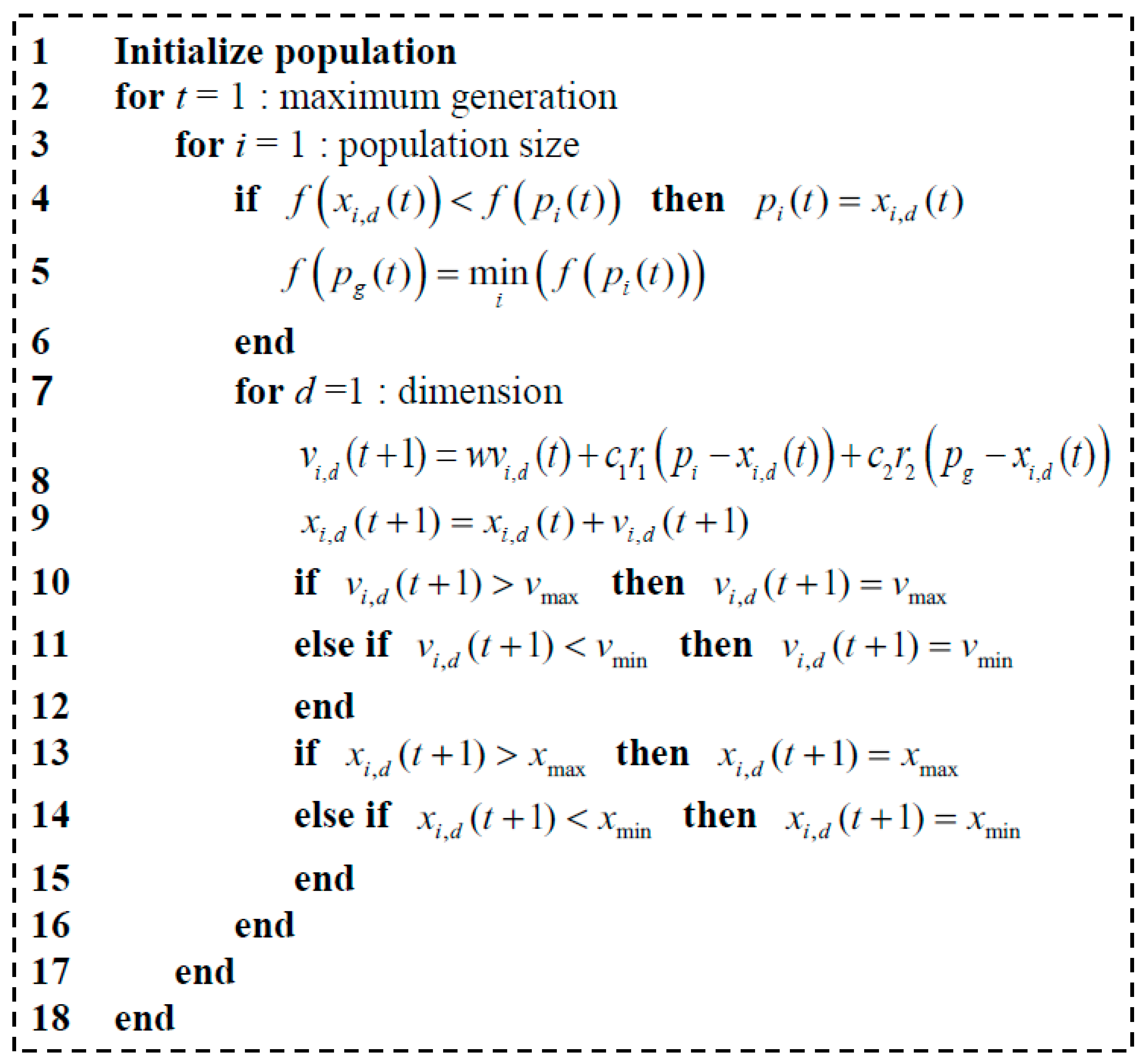
2.1. Standard Particle Swarm Optimization Algorithm

In standard PSO algorithm, each particle represents a potential solution to the task within the search space. In the D-dimensional space, the position vector and velocity vector of the ith particle can be expressed as $x_i=\left(x_{i1},x_{i2},\cdots ,x_{iD}\right)$ and $v_i=\left(v_{i1},v_{i2},\cdots ,v_{iD}\right)$, respectively. After the random initialization of particles, the velocity and position of the ith particle are updated as follow,

$$v_i(t+1)=w{v}_i(t)+c_1{r}_1\left(p_i-x_i(t)\right)+c_2{r}_2\left(p_g-x_i(t)\right)$$

(1)

$$x_i(t+1)=x_i(t)+v_i(t+1)$$

(2)

where, $w$ is the inertia weight and can be used to control the influence of previous velocity on the new one; the parameters $c_1$ and $c_2$ are two constants which determine the weights of $p_i$ and $p_g$; $p_i$ represents the best previous position of the ith individual and $p_g$ denotes the best previous position of all particles in current generation; $r_1$ and $r_2$ represent two separately generated random values which uniformly distribute in the range of [0, 1]. The pseudocode of standard particle swarm optimization is shown in Figure 1.

2.2. Modifications for Particle Swarm Optimization Algorithm

In the original studies of the PSO algorithm, the range of inertia weight ($w$) attracted researchers’ attention, and they suggested that the PSO algorithm with an inertia weight within the range of [0.9, 1.2] can take the least average number of iterations to find the global optimum [42]. In later research, the inertia weight adaptation mechanism is established to improve the global optimization ability of the PSO algorithm. Generally, the various inertia weighting strategies can be classified into three categories: (1) constant or random inertia weight strategies; (2) time varying inertia weight strategies; (3) adaptive inertia weight strategies.

2.2.1. Constant or Random Inertia Weight Strategies

The value of inertia weight is constant during the search or is determined randomly [20,43]. The impact of the inertia weight on the performance of the PSO algorithm is analyzed by Shi and Eberhart [20], and then they proposed a random inertia weight strategy for the PSO algorithm to track the optima in a dynamic environment, which can be expressed as,

$$w=0.5+\frac{r}{2}$$

(3)

where $r$ is a random value in [0, 1]. Then $w$ is a uniform random variable in the range of [0.5, 1].

2.2.2. Time Varying Inertia Weight Strategies

The inertia weight is defined as a function of time or iteration number [44,45,46]. In these strategies, the inertia weight can be updated in many ways. For example, the linear decreasing inertia weight can be expressed as [35,36],

$$w(iter)=\frac{ite{r}_{\max }-iter}{ite{r}_{\max }}\left(w_{\max }-w_{\min }\right)+w_{\min }$$

(4)

where $iter$ is the current iteration of algorithm and $ite{r}_{\max }$ represents the maximum number of iterations; $w_{\max }$ and $w_{\min }$ are the upper and lower bounds of inertia weight, and they are 0.9 and 0.4, respectively.

Based on the linear decreasing inertia weight strategy, the nonlinear decreasing strategy for inertia weight is proposed for the PSO algorithm [47], and it can be expressed as,

$$w(iter)={\left[\frac{ite{r}_{\max }-iter}{ite{r}_{\max }}\right]}^n\left(w_{\max }-w_{\min }\right)+w_{\min }$$

(5)

where $n$ is the nonlinear modulation index. Obviously, with $n=1$, this strategy becomes the linearly decreasing inertia weight strategy.

In addition, some similar methods [48,49,50,51], which use linear or nonlinear decreasing inertia weight, haven been proposed to improve the performance of the PSO algorithm.

2.2.3. Adaptive Inertia Weight Strategies

The inertia weight is adjusted by using one or more feedback parameters to balance the global and local searching abilities of the PSO algorithm [52,53,54,55]. These feedback parameters include the global best fitness, the local best fitness, the particle rank, and the distance to the global best position, etc.

In each iteration, the inertia weight determined by the ratio of the global best fitness and the average of particles’ local best fitness can be expressed as [17],

$$w(iter)=1.1-\frac{p_g(iter)}{\frac{1}{N}{\displaystyle \sum _{i=1}^N{p}_i(iter)}}$$

(6)

where $p_i(iter)$ and $p_g(iter)$ represent the best previous positions of the i-th individual and all particles, respectively; N is the number of particles.

The inertia weight updated by the particle rank can be expressed as [53],

$$w_i(iter)=w_{\min }+\frac{ran{k}_i}{N}\left(w_{\max }-w_{\min }\right)$$

(7)

where $w_i(iter)$ is the inertia weight of the i-th particle in current iteration; $ran{k}_i$ represents the position of the i-th particle when the particles are ordered based on their best fitness.

The inertia weight adjusted by the distance to the global best position can be expressed as [54],

$$w_i=w_0\left(1-\frac{dis{t}_i}{\max \_dist}\right)$$

(8)

where the inertia weight $w_0=rand(0.5,1)$; $dis{t}_i$ is the current Euclidean distance of the i-th particle from the global best, and it can be expressed as,

$$dis{t}_i={\left[{\displaystyle \sum _{d=1}^D{\left(p_g^d-x_i^d\right)}^2}\right]}^{\frac{1}{2}}$$

(9)

and $\max \_dist$ is the maximum distance of a particle from the global best in the previous generation.

In recent research, the PSO algorithm with inertia weight adjusted by the average absolute value of velocity or the situation of swarm is proposed to keep the balance between local search and global search [56,57,58]. In addition, the adaptive population size strategy is an effective way to improve the accuracy and efficiency of the PSO algorithm [59,60,61,62].

It is obvious that the improvements of the PSO algorithm are generally implemented by adaptively adjusting inertia weight or population size. These methods can avoid falling into local optima by adaptively updating the velocity of particle to some extent. However, the effect of random values on the particle velocity has never been discussed. Therefore, the PSO algorithm with different types of random values will be studied in Section 3 in detail.

3. Particle Swarm Optimization Algorithm with Different Types of Random Values

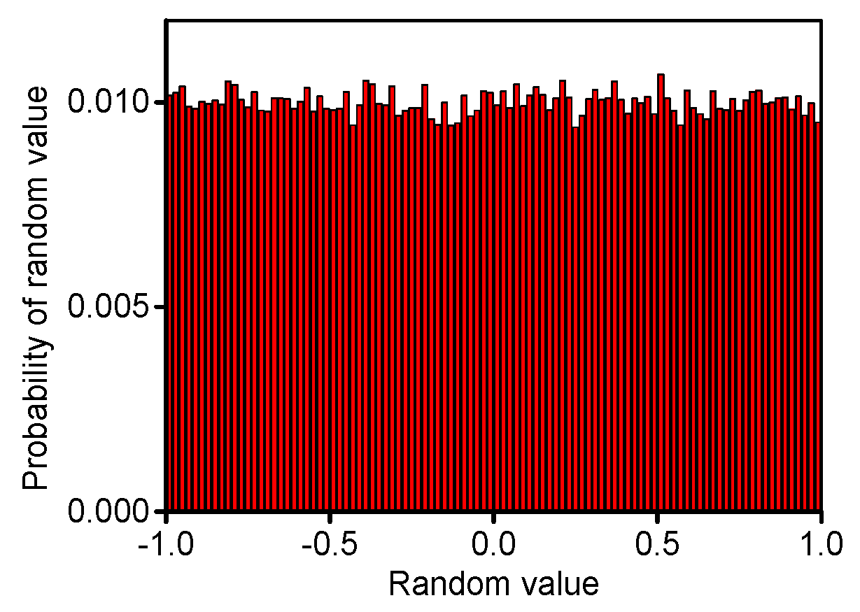
3.1. Random Values with Uniform Distribution in the Range of [0, 1]

In the traditional PSO algorithm, the random values $r_1$ and $r_2$ are generated by uniform distribution in the range of [0, 1] ($U\left[0,1\right]$). As shown in Figure 2, the probability of each random value is similar in the range.

3.2. Random Values with Uniform Distribution in the Range of [−1, 1]

In order to expand the range of random values, the random values $r_1$ and $r_2$ are generated by uniform distribution in the range of [−1, 1] ($U\left[-1,1\right]$) for the PSO algorithm. As shown in Figure 3, the probability of each random value is similar in the range.

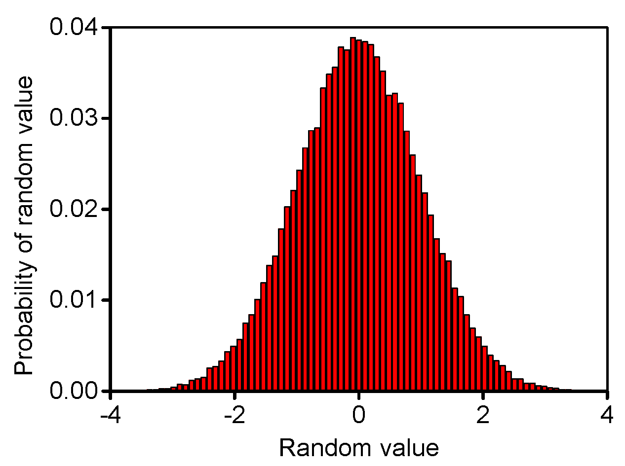
3.3. Random Values with Gauss Distribution

In order to expand the range of random values and change their probability, the random values $r_1$ and $r_2$ are generated by Gauss distribution with mean 0, and variance 1 ($G(0,1)$) for the PSO algorithm. As shown in Figure 4, the probability of each random value is different and symmetrically distributes about $r=0$. Furthermore, its probability is increased with decreasing the absolute value of random number.

4. Experiments and Analysis

4.1. Experimental Setup

In order to investigate the performances of PSO algorithms with different types of random values, some commonly used benchmark functions are adopted and shown in

Table 1. Benchmark functions.

Function Name	Test Function	Search Space	The Range of Particle Velocity	The Best Solution	The Best Result
Sphere1	$f_1(\mathrm{x})={\displaystyle \sum _{i=1}^D{x}_i^2}$	${\left[-100,100\right]}^D$	$\left[-100,100\right]$	$\left[0,\cdots ,0\right]$	0
Sphere2	$f_2(\mathrm{x})={\displaystyle \sum _{i=1}^D{x}_i^2}$	${\left[-10,190\right]}^D$	$\left[-10,10\right]$	$\left[0,\cdots ,0\right]$	0
Rastrigin	$f_3(x)={\displaystyle \sum _{i=1}^D\left(x_i^2-10\cos (2\pi x_i)+10\right)}$	${\left[-5.12,5.12\right]}^D$	$\left[-5.12,5.12\right]$	$\left[0,\cdots ,0\right]$	0
Rosenbrock	$f_4(x)={\displaystyle \sum _{i=1}^{D-1}\left(100{\left(x_{i+1}-x_i^2\right)}^2+{\left(x_i-1\right)}^2\right)}$	${\left[-30,30\right]}^D$	$\left[-30,30\right]$	$\left[1,\cdots ,1\right]$	0
Griewank	$f_5(x)=\frac{1}{4000}{\displaystyle \sum _{i=1}^D{x}_i^2-{\displaystyle \prod _{i=1}^D\cos \left(\frac{x_i}{\sqrt{i}}\right)}}+1$	${\left[-600,600\right]}^D$	$\left[-600,600\right]$	$\left[0,\cdots ,0\right]$	0
Ackley	$\begin{array}{ll}{f}_6(x)=& -20\exp \left(-0.2\sqrt{\frac{1}{30}{\displaystyle \sum _{i=1}^D{x}_i^2}}\right)\\ & -\exp \left(\frac{1}{D}{\displaystyle \sum _{i=1}^D\cos (2\pi x_i)}\right)+20+e\end{array}$	${\left[-32,32\right]}^D$	$\left[-32,32\right]$	$\left[0,\cdots ,0\right]$	0
Levy and Montalvo 2	$\begin{array}{ll}{f}_7(x)=& 0.1({\sin }^2\left(3\pi x_1\right)+{\displaystyle \sum _{i=1}^{D-1}{\left(x_i-1\right)}^2\left[1+{\sin }^2\left(3\pi x_{i+1}\right)\right]}\\ & +{\left(x_D-1\right)}^2\left[1+{\sin }^2\left(2\pi x_D\right)\right])\end{array}$	${\left[-5,5\right]}^D$	$\left[-5,5\right]$	$\left[1,\cdots ,1\right]$	0
Sinsolidal	$\begin{array}{ll}{f}_8(x)=& -[2.5{\prod }_{i=1}^D\sin \left(x_i-\frac{\pi }{6}\right)\\ & +{\prod }_{i=1}^D\sin \left(5\left(x_i-\frac{\pi }{6}\right)\right)]\end{array}$	${\left[0,\pi \right]}^D$	$\left[-\pi ,\pi \right]$	$\left[\frac{2}{3}\pi ,\cdots ,\frac{2}{3}\pi \right]$	−3.5
Rotated Expanded Scaffer	$\begin{array}{ll}F(x,y)& =0.5+\frac{{\sin }^2\left(\sqrt{x^2+y^2}\right)-0.5}{{\left(1+0.001\left(x^2+y^2\right)\right)}^2}\\ f_9\left(x\right)& =F\left(x_1,x_2\right)+F\left(x_2,x_3\right)+\cdots \\ & +F\left(x_{D-1},x_D\right)+F\left(x_D,x_1\right)\end{array}$	${\left[-100,100\right]}^D$	$\left[-100,100\right]$	$\left[0,\cdots ,0\right]$	0
Alpine	$f_1(\mathrm{x})={\displaystyle \sum _{i=1}^D\left|x_i\cdot \sin x_i+0.1x_i\right|}$	${\left[-9,7\right]}^D$	$\left[-7,7\right]$	$\left[0,\cdots ,0\right]$	0
Moved axis parallel hyper-ellipsoid	$f_1(\mathrm{x})={\displaystyle \sum _{i=1}^{D}5i\cdot x_i^2}$	${\left[-10,30\right]}^D$	$\left[-10,10\right]$	$\left[0,\cdots ,0\right]$	0
Schwefel	$f_1(\mathrm{x})={\displaystyle \sum _{i=1}^D\left[-x_i\cdot \sin (\sqrt{\left|x_i\right|})\right]}$	${\left[-300,500\right]}^D$	$\left[-300,300\right]$	$\left[\begin{array}{c}420.9687\\ ⋮\\ 420.9687\end{array}\right]$	$-D\cdot 418.9829$

. The dimensions of search space are 10, 30 and 100 in this study. The standard PSO algorithm is selected to investigate the effects of random values. In addition, because the linear decreasing inertia weight (LDIW) PSO algorithm has a better global search ability in starting phase to help the algorithm converge to an area quickly and a stronger local search ability in the latter phase to obtain high precision value, so the LDIW PSO algorithm is also utilized to study the effects of random values. Moreover, although the effects of setting parameters on deterministic PSO algorithm have been studied [63], the deterministic PSO algorithm (r = 0.5) is adopted to compare with standard PSO and LDIW-PSO algorithms.

To have a fair comparison, the parameter settings of all algorithms are same. In this study, the population size is 100, and the maximum number of function evaluations is 10,000. The parameters $c_1$ and $c_2$ are all 2. For standard PSO algorithm, the inertia weight $w$ is 0.7. For LDIW-PSO algorithm, $w_{\max }$ and $w_{\min }$ are 0.9 and 0.4, respectively. In order to eliminate random discrepancy, the results of all experiments are averaged over 30 independent runs.

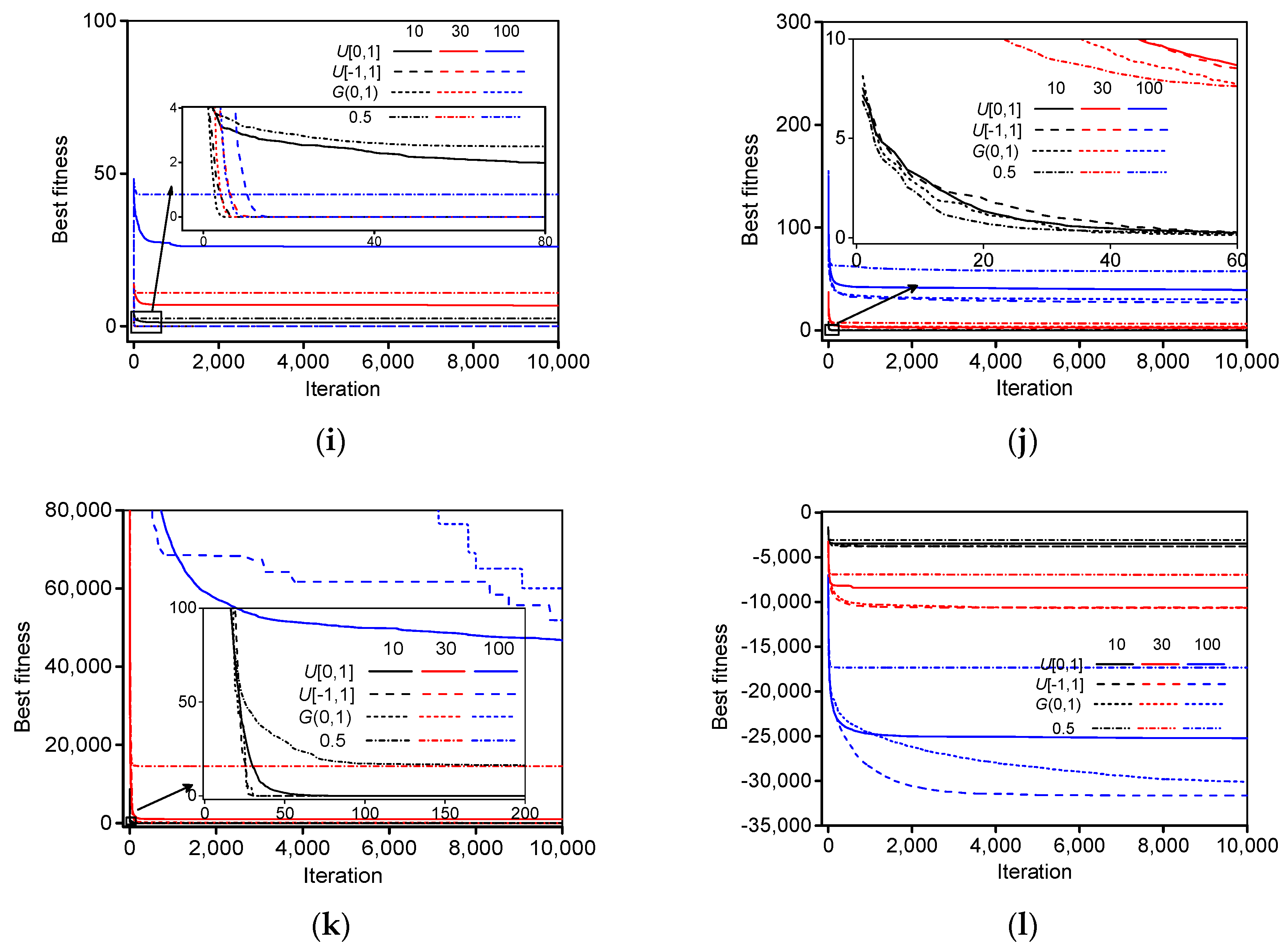
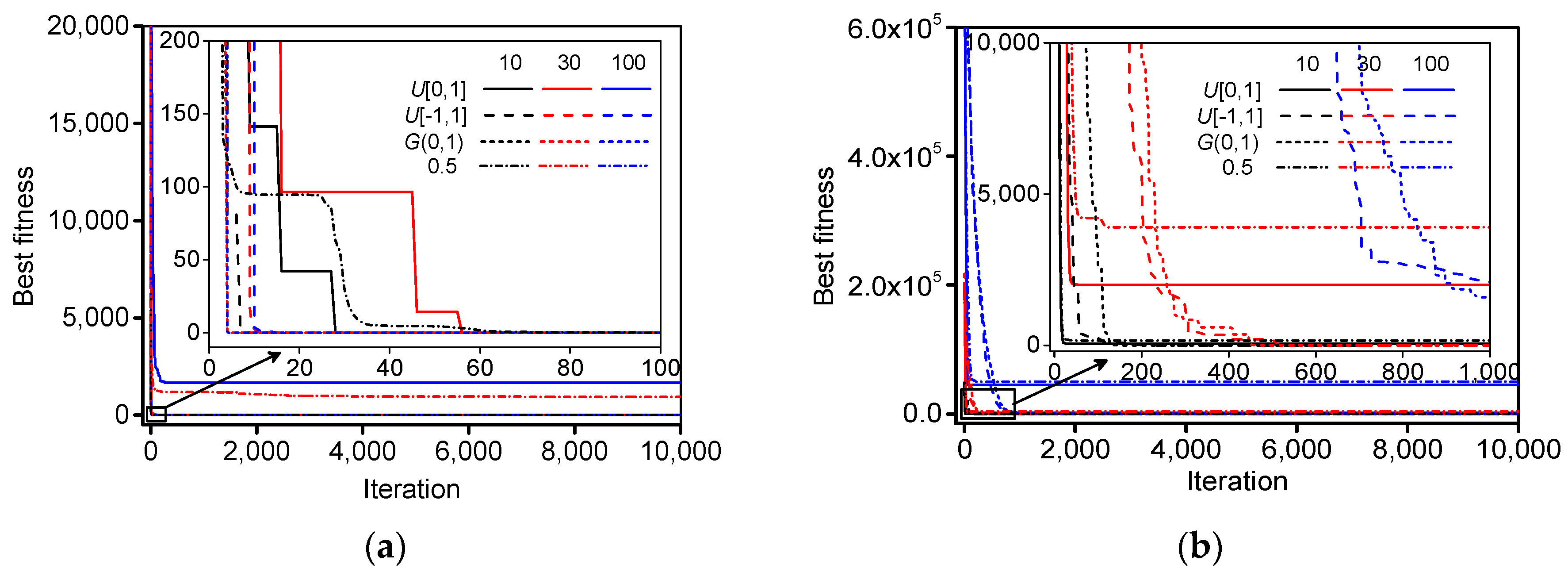
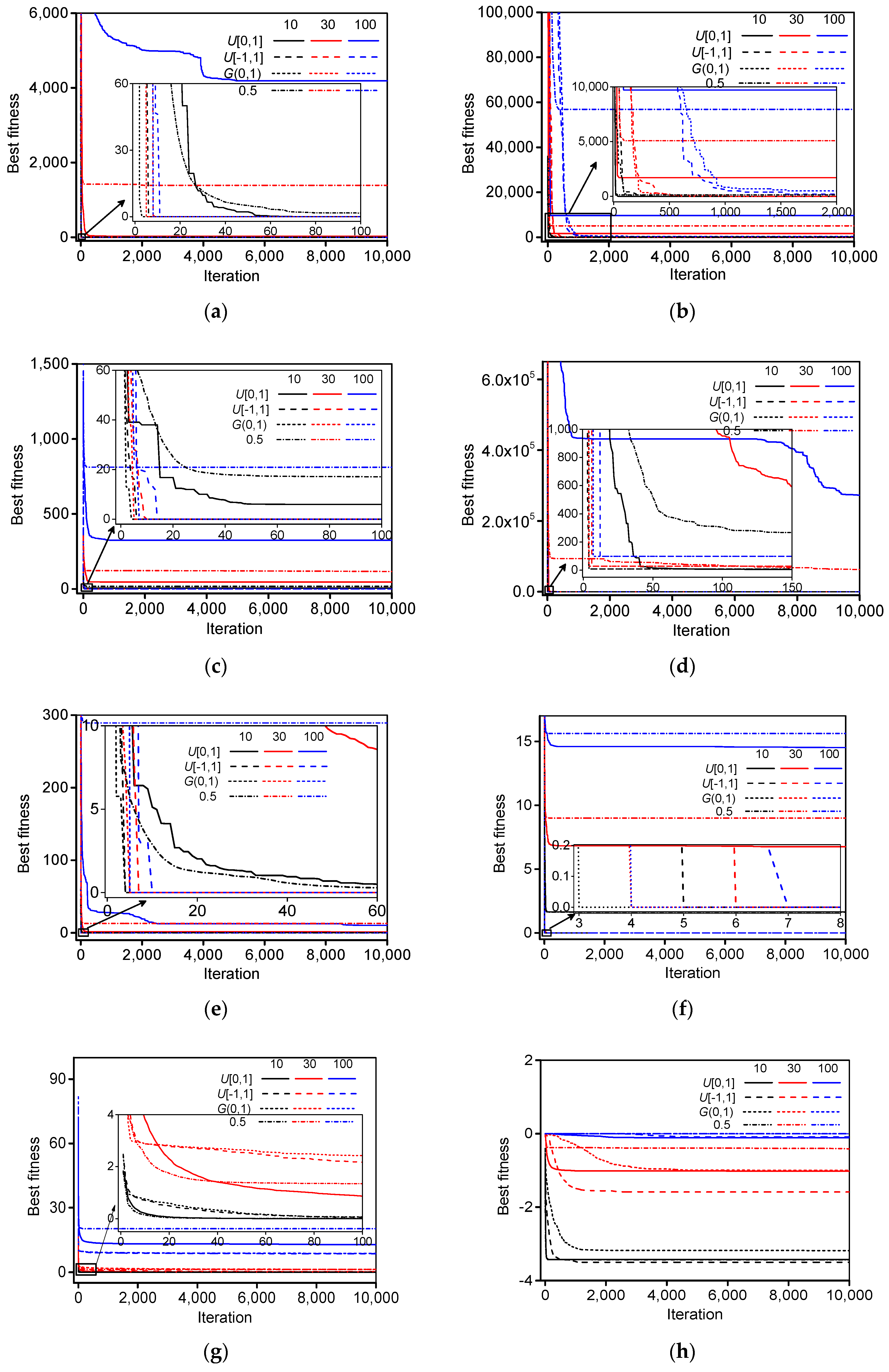
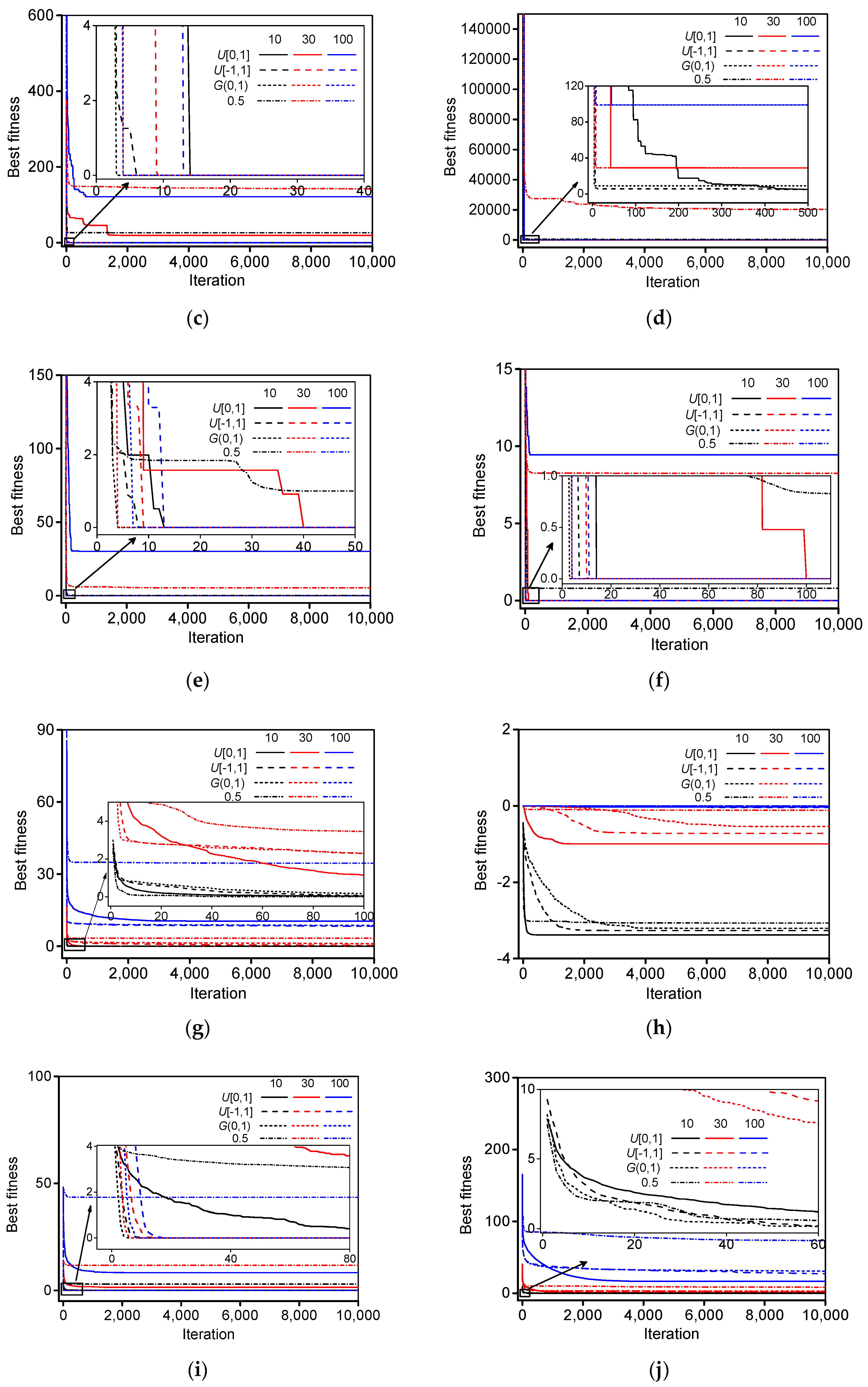
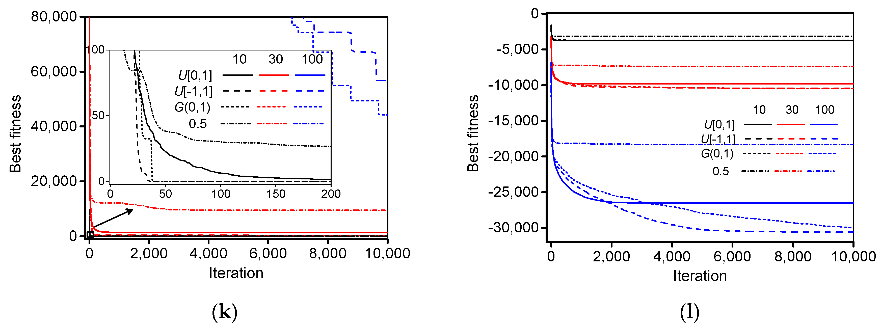
4.2. Experimental Results and Comparisons

For some benchmark functions, the comparisons of standard PSO algorithm with different types of random values are shown in

Table 2. Comparisons of standard particle swarm optimization (PSO) algorithm with different types of random values for benchmark functions.

Function	r1, r2	$\mathit{U}\left[0,1\right]$	0.5	$\mathit{U}\left[-1,1\right]$	$\mathit{G}(0,1)$
	Dimension	10/30/100	10/30/100	10/30/100	10/30/100
Sphere1	Average solution	0/19.90/4203.68	0.74/1390.12/34,069.52	0/0/0	0/0/0
	Standard deviation	0/12.37/4400.60	1.62/575.44/10,343.18	0/0/0	0/0/0
	The worst solution	0/48.87/13,080.62	7.90/2730.92/53,024.46	0/0/0	0/0/0
	The best solution	0/4.13/303.05	0/443.08/17,579.98	0/0/0	0/0/0
Sphere2	Average solution	0/1726.67/9386.74	130.34/5076.33/56,870.86	0/0/183.33	0/0/220
	Standard deviation	0/466.04/6716.49	180.26/9114.11/75,788.47	0/0/159.92	0/0/174.99
	The worst solution	0/2600/44,700	600/38,700/323,027.84	0/0/600	0/0/600
	The best solution	0/900.00/6400.80	0.01/2319.72/9236.02	0/0/0	0/0/0
Rastrigin	Average solution	1.03/52.83/357.43	17.01/116.61/810.69	0/0/0	0/0/0
	Standard deviation	1.60/21.87/81.84	9.70/33.22/76.28	0/0/0	0/0/0
	The worst solution	4.97/100.77/499.92	42.81/215.88/932.59	0/0/0	0/0/0
	The best solution	0/3.62/186.01	4.98/62.26/670.46	0/0/0	0/0/0
Rosenbrock	Average solution	0.40/462.38/308,982.29	250.36/63,215/13,665,740.29	1.93/28.86/98.92	0.98/28.90/98.94
	Standard deviation	1.22/292.83/182,460.39	663.05/59,859/6,367,792.97	2.86/0.08/0.05	2.43/0.07/0.03
	The worst solution	3.99/1383.17/874,057.21	3515.43/260,355.55/27,517,029.65	8.93/28.96/98.98	8.75/28.97/98.98
	The best solution	0/165.84/36,093.44	5.86/1614.69/5,391,184.05	0.00/28.67/98.77	1.63 × 10−6/28.69/98.86
Griewank	Average solution	0.19/1.13/17.27	0.22/12.88/289.00	0/0/0	0/0/0
	Standard deviation	0.15/0.15/9.06	0.12/5.64/84.70	0/0/0	0/0/0
	The worst solution	0.51/1.51/39.44	0.59/26.48/519.72	0/0/0	0/0/0
	The best solution	0/0.90/3.45	0.08/3.34/123.68	0/0/0	0/0/0
Ackley	Average solution	1.46/6.07/11.12	1.64/9.00/15.63	0/0/0	0/0/0
	Standard deviation	1.22/1.50/2.26	1.02/1.25/1.10	0/0/0	0/0/0
	The worst solution	3.22/8.90/15.17	3.58/12.06/17.46	0/0/0	0/0/0
	The best solution	0/2.73/3.44	0.02/6.98/13.44	0/0/0	0/0/0
Levy and Montalvo 2	Average solution	0/0.14/12.83	0.01/1.31/20.28	0/0.23/8.63	0/1.34/8.78
	Standard deviation	0/0.17/2.31	0.01/0.54/4.57	0/0.46/0.48	0/0.64/0.44
	The worst solution	0/0.81/17.84	0.06/2.78/34.78	0/1.60/9.42	0/2.49/9.57
	The best solution	0/0.01/9.09	0.00/0.28/14.28	0/0/7.38	0/0/7.89
Sinsolidal	Average solution	−3.43/−1.02/−0.11	−3.43/−0.41/0	−3.50/−1.59/−0.09	−3.18/−1/0
	Standard deviation	0.29/1.14/0.31	0.14/0.46/0	0/1.56/0.32	0.74/1.18/0
	The worst solution	−2.12/−0.01/0	−2.93/−0.01/0	−3.50/−0.01/0	−0.87/−0.01/0
	The best solution	−3.50/−3.45/−1.66	−3.50/−1.47/0	−3.50/−3.50/−1.75	−3.50/−3.50/0
Rotated Expanded Scaffer	Average solution	1.27/6.77/26.10	2.58/10.92/43.13	0/0/0	0/0/0
	Standard deviation	0.74/1.96/5.54	0.47/1.18/1.59	0/0/0	0/0/0
	The worst solution	2.60/9.24/34.49	3.56/13.11/45.81	0/0/0	0/0/0
	The best solution	0/1.92/13.45	1.73/8.63/39.45	0/0/0	0/0/0
Alpine	Average solution	0/2.67/39.15	0.12/6.36/57.50	0/2.14/27.04	0/3.36/30.12
	Standard deviation	0/1.70/8.56	0.34/1.81/8.48	0/1.17/3.96	0/1.19/3.65
	The worst solution	0/7.30/62.51	1.81/10.83/75.846	0/5.71/34.30	0/6.04/38.17
	The best solution	0/0.27/17.71	0/2.94/44.30	0/0/16.87	0/1/23.11
Moved axis parallel hyper-ellipsoid	Average solution	0/976.19/102,196.49	10.66/14,535.57/714,363.54	0/0/56,727.35	0/0/44,270.31
	Standard deviation	0/2276.36/46,700.85	21.97/6358.06/125,266.58	0/0/54,460.61	0/0/70,284.76
	The worst solution	0/8532.57/196,643.04	105.74/33,237.39/967,098.52	0/0/195,537.54	0/0/235,721.53
	The best solution	0/7.13/21,301.13	0.01/5625.85/484,347.13	0/0/0	0/0/0
Schwefel	Average solution	−3472.55/−8400.88/−25,222.99	−3072.44/−6957.38/−17,338.78	−3772.47/−10,596.14/−31,640.44	−3772.47/−10,651.80/−30,094.87
	Standard deviation	301.97/862.61/2717.54	402.88/941.95/2511.55	229.58/745.71/2489.84	233.82/635.86/1790.82
	The worst solution	−2865.61/−6560.66/−20,423.87	−2151.57/−4665.91/−12,121.78	−3355.12/−9101.35/−25,385.62	−3235.87/−9101.35/−26,155.70
	The best solution	−4070.58/−9946.11/−31,017.18	−3733.40/−8648.21/−21,643.45	−4189.83/−11,854.02/−37,370.87	−4189.83/−11,854.01/−32,695.87

. The bold numbers indicate the best solutions for each test function in the certain space dimension. Obviously, the performances of deterministic PSO algorithm (r = 0.5) are the worst for all the benchmark functions. This is because the random values are deterministic which decreases the diversity of particles. For the random values generated by $U\left[0,1\right]$,the standard PSO algorithm can only obtain the optimal solutions of Sphere1, Sphere2, Alpine and Moved axis parallel hyper-ellipsoid when the space dimension is 10, but this algorithm is useless for other test functions or higher space dimensions. However, for the random values generated by $U\left[-1,1\right]$ or $G(0,1)$, the standard PSO algorithm can obtain the optimal solutions of all test functions in every space dimension except Rosenbrock. In the low space dimension (10), the best solution of Rosenbrock is obtained by the standard PSO algorithm with random values distributed in $U\left[0,1\right]$. However, in the high space dimension (30 or 100), its best solution is obtained by the standard PSO algorithm with random values generated by $U\left[-1,1\right]$ or $G(0,1)$. In addition, the best solutions of Levy and Montalvo 2 (30 dimensions) and Sinusoidal (100 dimensions) are also obtained by the standard PSO algorithm with random values distributed in $U\left[0,1\right]$. Obviously, the random values make an important effect on the performance of standard PSO algorithm, and its performance is highly improved when the range of random value is expanded. This implies that the standard PSO algorithm with large-scale random values can avoid falling into local optima and obtain the global optima.

The comparisons of LDIW-PSO algorithm with different types of random values for benchmark functions are shown in

Table 3. Comparisons of LDIW-PSO algorithm with different types of random values for benchmark functions.

Function	r1, r2	$\mathit{U}\left[0,1\right]$	0.5	$\mathit{U}\left[-1,1\right]$	$\mathit{G}(0,1)$
	Dimension	10/30/100	10/30/100	10/30/100	10/30/100
Sphere1	Average solution	0/0/1666.67	0/937.89/62,668.95	0/0/0	0/0/0
	Standard deviation	0/0/4611.33	0.01/1954.53/19,933.81	0/0/0	0/0/0
	The worst solution	0/0/20,000	0.04/8616.07/110,110.64	0/0/0	0/0/0
	The best solution	0/0/0	0/62.99/35,629.65	0/0/0	0/0/0
Sphere2	Average solution	56.67/2033.33 /46,393.33	151.13/3905.81/49,939.96	0/0/293.33	0/0/236.6667
	Standard deviation	67.89/256.41/35,977.84	122.87/6591.85/40,171.84	0/0/228.84	0/0/225.1181
	The worst solution	200/2600/189,200	500.38/38,800/153,700	0/0/900	0/0/700
	The best solution	0/1600/8600	0.03/2361.29/9103.90	0/0/0	0/0/0
Rastrigin	Average solution	0/18.90 /130.24	26.30/142.34/865.88	0/0/0	0/0/0
	Standard deviation	0/22.91/83.07	11.70/31.11/82.15	0/0/0	0/0/0
	The worst solution	0/82.72/335.59	48.75/193.01/1096.66	0/0/0	0/0/0
	The best solution	0/0/28.92	7.97/67.63/737.39	0/0/0	0/0/0
Rosenbrock	Average solution	0.27/26.04/98.15	379.22/20,307.62/33,690,571.22	0.47/28.81/98.87	2.39/28.90/98.93
	Standard deviation	1.01/0.54/0.08	845.50/34,257.18/41,367,235.20	1.54/0.09/0.04	3.33/0.06/0.04
	The worst solution	3.99/27.30/98.24	3032.11/107,129.05/231,274,237.32	7.48/28.94/98.94	8.95/28.98/98.99
	The best solution	0/25.04/97.89	4.96/1698.53/6,545,833.08	0/28.59/98.77	1.29 × 10−8/28.76/98.79
Griewank	Average solution	0/0/28.04	0.19/5.28/478.06	0/0/0	0/0/0
	Standard deviation	0/0/42.54	0.18/3.19/155.18	0/0/0	0/0/0
	The worst solution	0/0/90.93	0.84/14.45/941.53	0/0/0	0/0/0
	The best solution	0/0/0	0.05/1.70/203.77	0/0/0	0/0/0
Ackley	Average solution	0/0/9.64	0.80/8.25/18.27	0/0/0	0/0/0
	Standard deviation	0/0/6.53	0.85/2.90/0.79	0/0/0	0/0/0
	The worst solution	0/0/19.97	2.81/16.67/19.44	0/0/0	0/0/0
	The best solution	0/0/0	0/4.40/16.92	0/0/0	0/0/0
Levy and Montalvo 2	Average solution	0/0/10.48	0/3.35/34.54	0/0.36/8.28	0/1.08/8.64
	Standard deviation	0/0/3.20	0/1.84/8.01	0/0.50/0.62	0/0.68/0.37
	The worst solution	0/0/17.73	0/7.62/49.10	0/1.51/9.37	0/2.20/9.32
	The best solution	0/0/5.40	0/0.70/18.90	0/0/6.31	0/0/7.70
Sinsolidal	Average solution	−3.38/−1/−0.03	−3.07/−0.12/0	−3.27/−0.72/−0.05	−3.21/−0.54/0
	Standard deviation	0.44/1.13/0.09	0.53/0.16/0	0.61/1.02/0.18	0.66/0.80/0
	The worst solution	−1.75/0/0	−1.75/0/0	−1.75/0/0	−1.75/0/0
	The best solution	−3.50/−3.50/−0.44	−3.50/−0.70/0	−3.50/−3.50/−0.87	−3.50/−3.50/0
Rotated Expanded Scaffer	Average solution	0.07/1.44/8.33	3/11.74/43.49	0/0/0	0/0/0
	Standard deviation	0.25/1.49/3.53	0.47/1.03/1.02	0/0/0	0/0/0
	The worst solution	1/5.98/14.94	3.70/12.97/46.10	0/0/0	0/0/0
	The best solution	0/0/0	1.42/8.57/41.56	0/0/0	0/0/0
Alpine	Average solution	0/0.91/16.46	0.31/8.41/73.22	0/2.45/27.24	0/2.93/30.70
	Standard deviation	0/1.94/7.65	0.76/3.95/13.39	0/1.23/6.95	0/1.44/4.19
	The worst solution	0/8.46/34.94	2.85/15.54/96.89	0/5.02/36.40	0/6.16/37.74
	The best solution	0/0.02/5.71	0/1.08/48.66	0/0/0	0/1/22.49
Moved axis parallel hyper-ellipsoid	Average solution	0/1383.33/102,196.49	20.64/9487.68/714,363.54	0/265.79/56,727.35	0/132.76/44,270.31
	Standard deviation	0/2215.48/46,700.85	90.81/5798.05/125,266.58	0/865.18/54,460.61	0/727.13/70,284.76
	The worst solution	0/7000/196,643.04	500/24,372.80/967,098.52	0/3982.80/195,537.54	0/3982.65/235,721.53
	The best solution	0/0/21,301.13	0/2221.47/484,347.13	0/0/0	0/0/0
Schwefel	Average solution	−3764.52/−9823.92/−26,540.45	−3134.09/−7401.16/−18,304.47	−3764.52/−10,431.89/−30,589.24	−3732.73/−10,492.05/−29,986.84
	Standard deviation	142.42/1344.37/3360.98	450.61/794.06/2000.45	243.94/662.12/2767.91	226.00/698.81/2431.96
	The worst solution	−3474.36/−6944.90/−20,227.96	−2057.33/−5583.79/−14,272.03	−3235.87/−8743.62/−25,650.73	−3235.87/−8624.37/−25,743.44
	The best solution	−3951.34/−11,854.02/−31,935.70	−3832.10/−9056.25/−22,371.46	−4189.83/−11,496.29/−37,956.42	−4189.83/−11,948.07/−34,477.94

. In addition, the bold numbers indicate the best solutions for each test function in the certain space dimension. For all the benchmark functions, the performances of deterministic LDIW-PSO algorithm (r = 0.5) are also the worst. For the $U\left[-1,1\right]$ and $G(0,1)$, the performance of LDIW-PSO algorithm is similar with that of standard PSO algorithm. However, for the random values distributed in $U\left[0,1\right]$, the performance of LDIW-PSO algorithm is improved compared to the standard PSO algorithm, which is also reported in some references [5,20,45,46]. It should be noted that the LDIW-PSO algorithm with random values generated by $U\left[0,1\right]$ can obtain the optimal solutions of all test function in low space dimension (10 and 30) except Sphere2, Rotated Expanded Scaffer and Schwefel. In addition, for Levy and Montalvo 2, Sinusoidal and Alpine in 30 dimensions, the performance of LDIW-PSO algorithm with random values generated by $U\left[0,1\right]$ is better than that with random values generated by $U\left[-1,1\right]$ or $G(0,1)$. However, in the high space dimension (100), the LDIW-PSO algorithm with random values generated by $U\left[0,1\right]$ cannot obtain the optimal solutions of these test functions, which implies that this algorithm is useless for the problems in high dimension space. Therefore, the performance of improved PSO (LDIW-PSO) algorithm is also influenced by the random values, especially for solving the problems in high dimension space. Furthermore, the LDIW-PSO algorithm with a wide range of random values is more beneficial to escape from local optima and obtain the global optima.

Figure 5 shows the mean best fitness of the standard PSO algorithm with different types of random values for benchmark functions. For the same type of random values, the performance of the standard PSO algorithm improves with decreasing the space dimension, and the convergence velocity also improves with decreasing the space dimension. For the same space dimension of each test function, the performances of deterministic PSO algorithm (r = 0.5) are the worst. However, the performances of standard PSO algorithm with random values generated by $U\left[-1,1\right]$ or $G(0,1)$ are the best for the most benchmark functions. In the low dimension (10 and 30), the performances of standard PSO algorithm with random values generated by $U\left[0,1\right]$ and $U\left[-1,1\right]$ are the best for Levy and Montalvo 2 and Sinusoidal, respectively. The performance of the standard PSO algorithm with random values distributed in $U\left[-1,1\right]$ is slightly worse than that of the standard PSO algorithm with random values distributed in $G(0,1)$. In addition, the global optima can be obtained within 50 iterations by the standard PSO algorithm with random values generated by $U\left[-1,1\right]$ or $G(0,1)$. This indicates that the standard PSO algorithm with large-scale random values can more quickly obtain the global optima.

The mean best fitness of the LDIW-PSO algorithm with different types of random values for benchmark functions are shown in Figure 6. In addition, the performance and convergence velocity of the LDIW-PSO algorithm are all improved with decreasing the space dimension for the same random values of each test function. When the random values are generated by $U\left[0,1\right]$, compared to the standard PSO algorithm, the LDIW-PSO algorithm has better performance. In the space dimensions 10 and 30, the global optima of some test functions can be obtained by the LDIW-PSO algorithm with random values are generated by $U\left[0,1\right]$, but its convergence velocity is slower than that of the LDIW-PSO algorithm with random values generated by $U\left[-1,1\right]$ or $G(0,1)$. Moreover, in the low dimension (10 and 30), the performance of the LDIW-PSO algorithm with random values generated by $U\left[0,1\right]$ is the best for Levy and Montalvo 2, Sinusoidal and Alpine. When the space dimension is 100, the global optima cannot be obtained by the LDIW-PSO algorithm with random values distributed in $U\left[0,1\right]$, but can be obtained by the LDIW-PSO algorithm with random values distributed in $U\left[-1,1\right]$ or $G(0,1)$. This implies that the LDIW-PSO algorithm with large-scale random values can be more likely to obtain the global optima with less iterations.

4.3. Application and Analysis

4.3.1. Application in Engineering Problem

The pressure vessel design, which was initially introduced by Sandgren [64], is a real world engineering problem. There are four involved variables, including the thickness (x₁), thickness of the head (x₂), the inner radius (x₃), and the length of the cylindrical section of the vessel (x₄). The highly constrained problem of pressure vessel design can be expressed as,

$$\mathrm{Min}:f(x)=0.6224x_1{x}_3{x}_4+1.7781x_2{x}_3^2+3.1611x_1^2{x}_4+19.84x_2^2{x}_4$$

(10)

$$\begin{array}{ll}\mathrm{Subject}\mathrm{to}:& \\ & {\mathrm{g}}_1=0.0163x_3-x_1\le 0,\\ & {\mathrm{g}}_2=0.00954x_3-x_2\le 0,\\ & {\mathrm{g}}_3=1296000-\pi x_3^2{x}_4-\frac{4}{3}\pi x_3^3\le 0,\\ & {\mathrm{g}}_4=x_4-240\le 0,\\ & {\mathrm{g}}_5=1.1-x_1\le 0,\\ & {\mathrm{g}}_6=0.6-x_2\le 0.\end{array}$$

(11)

where x₁ and x₂ are integer multipliers of 0.0625. x₃ and x₄ are continuous variables in the ranges of 40 ≤ x₃ ≤ 80 and 20 ≤ x₄ ≤ 60. In this study, the standard PSO and LDIW-PSO algorithms with different types of random values are utilized to solve this engineering problem.

The parameters of standard PSO and LDIW-PSO algorithms for the engineering problem are the same as those for benchmark functions. In order to eliminate random discrepancy, the results are averaged over 30 independent runs. The optimization results are shown in

Table 4. Comparisons of standard PSO and LDIW-PSO algorithms with different types of random values for pressure vessel design.

Type	r1, r2	$\mathit{U}\left[0,1\right]$	0.5	$\mathit{U}\left[-1,1\right]$	$\mathit{G}(0,1)$
SPSO	Average solution	5975.93	5975.93	5975.93	5975.94
	Standard deviation	0.00	0.00	0.01	0.01
	The worst solution	5975.93	5975.93	5975.96	5975.99
	The best solution	5975.93	5975.93	5975.93	5975.93
LDIW-PSO	Average solution	5975.93	5975.93	6001.34	6026.76
	Standard deviation	0.00	0.00	139.18	193.41
	The worst solution	5975.93	5975.93	6738.24	6738.26
	The best solution	5975.93	5975.93	5975.93	5975.93

. Obviously, the results of all algorithms are similar. However, the performances of LDIW-PSO algorithm random values generated by $U\left[-1,1\right]$ and $G(0,1)$ are slightly poorer than those of other algorithms. This is because the pressure vessel design is a low dimensional optimization problem. Although the random values generated by $U\left[-1,1\right]$ or $G(0,1)$ are beneficial to improve the diversity of particles, the local searching ability may be decreased due to the finite particles.

4.3.2. Analysis

According to the experimental results and comparisons, it can be concluded that the performances of standard PSO and LDIW-PSO algorithms are all highly improved by expanding the range of random values. This is because that the large-scale random values are helpful in increasing the velocity of particles, and then the particles avoid falling into the local optima. As shown in Figure 7, in the local optima areas (A or C), if the velocity cannot be increased or its direction cannot be changed, the particle will gradually fall into the local optima and cannot jump out. However, if the velocity of particle can be increased or changed according to a certain probability, the global optima will be obtained more easily and quickly.

For the standard PSO and LDIW-PSO algorithms, if the random values are set as 0.5 or generated by $U\left[0,1\right]$, the diversity of particle is decreased, and the variation range of particle velocity is limited in a narrow band. Therefore, the probability of escaping local optima is very small. This is because the particle velocity gradually tends to 0 when the particle falls into local optima. In addition, the random value is a positive/negative number, which may lead to the monotonous variation of particle velocity. This also decreases the possibility of escaping local optima. However, the PSO algorithms with large-scale random values (distributed in $U\left[-1,1\right]$ or $G(0,1)$) can overcome these problems to some extent. Furthermore, for a low dimensional practical optimization problem, the random values generated by $U\left[-1,1\right]$ or $G(0,1)$ can improve the diversity of particles, but the local searching ability may be decreased due to the finite particles. However, keeping the balance between local search and global search is very important for the performances of these PSO algorithms. So, the PSO algorithm with random values distributed in $U\left[0,1\right]$ and deterministic PSO algorithm (r = 0.5) have better local searching ability for some low dimensional optimization problems.

5. Conclusions

In this paper, the standard PSO algorithm and one of its modifications (LDIW-PSO algorithm) are adopted to study and analyze the influences of random values generated by uniform distribution in the ranges of [0, 1] and [−1, 1], Gauss distribution with mean 0 and variance 1 ($U\left[0,1\right]$, $U\left[-1,1\right]$ and $G(0,1)$). In addition, the deterministic PSO algorithm, in which the random values are set as 0.5, is also investigated in this study. Some benchmark functions and the pressure vessel design problem are utilized to test and compare the performances of two PSO algorithms with different types of random values in three space dimensions (10, 30, and 100). The experimental results show that the performances of deterministic PSO algorithms are the worst. Moreover, the performances of two PSO algorithms with random values generated by $U\left[-1,1\right]$ or $G(0,1)$ are much better than that of the algorithms with random values generated by $U\left[0,1\right]$ for most benchmark functions. In addition, the convergence velocities of the algorithms with random values distributed in $U\left[-1,1\right]$ or $G(0,1)$ are much faster than that of the algorithms with random values distributed in $U\left[0,1\right]$. It is concluded that the PSO algorithms with large-scale random values can effectively avoid falling into the local optima and quickly obtain the global optima. However, for a low dimensional practical optimization problem, the random values generated by $U\left[-1,1\right]$ or $G(0,1)$ are beneficial to improve the global searching ability, but the local searching ability may be decreased due to the finite particles.

References

1. Kennedy, J.; Eberhart, R.C. Particle swarm optimization. In Proceedings of the IEEE International Conference on Neuron Networks, Perth, WA, Australia, 27 November–1 December 1995; pp. 1942–1948. [Google Scholar]
2. Wang, Y.; Li, B.; Weise, T.; Wang, J.Y.; Yuan, B.; Tian, Q.J. Self-adaptive learning based particle swarm optimization. Inf. Sci. 2011, 180, 4515–4538. [Google Scholar] [CrossRef]
3. Liang, J.J.; Qin, A.K.; Suganthan, P.N.; Baskar, S. Comprehensive learning particleswarm optimizer for global optimization of multimodal functions. IEEE Trans. Evol. Comput. 2006, 10, 281–295. [Google Scholar] [CrossRef]
4. Chen, D.B.; Zhao, C.X. Particle swarm optimization with adaptive population size and its application. Appl. Soft Comput. 2009, 9, 39–48. [Google Scholar] [CrossRef]
5. Xu, G. An adaptive parameter tuning of particle swarm optimization algorithm. Appl. Math. Comput. 2013, 219, 4560–4569. [Google Scholar] [CrossRef]
6. Mirjalili, S.A.; Hashim, S.Z.M.; Sardroudi, H.M. Training feedforward neural networks using hybrid particle swarm optimization and gravitational search algorithm. Appl. Math. Comput. 2012, 218, 11125–11137. [Google Scholar] [CrossRef]
7. Ren, C.; An, N.; Wang, J.; Li, L.; Hu, B.; Shang, D. Optimal parameters selection for BP neural network based on particle swarm optimization: A case study of wind speed forecasting. Knowl. Based Syst. 2014, 56, 226–239. [Google Scholar] [CrossRef]
8. Zhang, J.R.; Zhang, J.; Lok, T.M.; Lyu, M.R. A hybrid particle swarmoptimization–back-propagation algorithm for feedforward neural network training. Appl. Math. Comput. 2007, 185, 1026–1037. [Google Scholar]
9. Das, G.; Pattnaik, P.K.; Padhy, S.K. Artificial Neural Network trained by Particle Swarm Optimization for non-linear channel equalization. Expert Syst. Appl. 2014, 41, 3491–3496. [Google Scholar] [CrossRef]
10. Lin, C.J.; Chen, C.H.; Lin, C.T. A hybrid of cooperative particle swarm optimization and cultural algorithm for neural fuzzy networks and its prediction applications. IEEE Trans. Syst. Man Cybern. Part C Appl. Rev. 2009, 39, 55–68. [Google Scholar]
11. Juang, C.F.; Hsiao, C.M.; Hsu, C.H. Hierarchical cluster-based multispecies particle-swarm optimization for fuzzy-system optimization. IEEE Trans. Fuzzy Syst. 2010, 18, 14–26. [Google Scholar] [CrossRef]
12. Kuo, R.J.; Hong, S.Y.; Huang, Y.C. Integration of particle swarm optimization-based fuzzy neural network and artificial neural network for supplier selection. Appl. Math. Model. 2010, 34, 3976–3990. [Google Scholar] [CrossRef]
13. Tang, Y.; Ju, P.; He, H.; Qin, C.; Wu, F. Optimized control of DFIG-based wind generation using sensitivity analysis and particle swarm optimization. IEEE Trans. Smart Grid 2013, 4, 509–520. [Google Scholar] [CrossRef]
14. Sui, X.; Tang, Y.; He, H.; Wen, J. Energy-storage-based low-frequency oscillation damping control using particle swarm optimization and heuristic dynamic programming. IEEE Trans. Power Syst. 2014, 29, 2539–2548. [Google Scholar] [CrossRef]
15. Jiang, H.; Kwong, C.K.; Chen, Z.; Ysim, Y.C. Chaos particle swarm optimization and T–S fuzzy modeling approaches to constrained predictive control. Expert Syst. Appl. 2012, 39, 194–201. [Google Scholar] [CrossRef]
16. Moharam, A.; El-Hosseini, M.A.; Ali, H.A. Design of optimal PID controller using hybrid differential evolution and particle swarm optimization with an aging leader and challengers. Appl. Soft Comput. 2016, 38, 727–737. [Google Scholar] [CrossRef]
17. Arumugam, M.S.; Rao, M.V.C. On the improved performances of the particle swarm optimization algorithms with adaptive parameters, cross-over operators and root mean square (RMS) variants for computing optimal control of a class of hybrid systems. Appl. Soft Comput. 2008, 8, 324–336. [Google Scholar] [CrossRef]
18. Pehlivanoglu, Y.V. A new particle swarm optimization method enhanced with a periodic mutation strategy and neural networks. IEEE Trans. Evolut. Comput. 2013, 17, 436–452. [Google Scholar] [CrossRef]
19. Ratnaweera, A.; Halgamuge, S.; Waston, H. Self-organizing hierarchical particle optimizer with time-varying acceleration coefficients. IEEE Trans. Evol. Comput. 2004, 8, 240–255. [Google Scholar] [CrossRef]
20. Shi, Y.H.; Eberhart, R.C. A modified particle swarm optimizer. In Proceedings of the IEEE International Conference on Computational Intelligence, Anchorage, AK, USA, 4–9 May 1998; pp. 69–73. [Google Scholar]
21. Xing, J.; Xiao, D. New Metropolis coefficients of particle swarm optimization. In Proceedings of the IEEE Chinese Control and Decision Conference, Yantai, China, 2–4 July 2008; pp. 3518–3521. [Google Scholar]
22. Taherkhani, M.; Safabakhsh, R. A novel stability-based adaptive inertia weight for particle swarm optimization. Appl. Soft Comput. 2016, 38, 281–295. [Google Scholar] [CrossRef]
23. Nickabadi, A.; Ebadzadeh, M.M.; Safabakhsh, R. A novel particle swarm optimization algorithm with adaptive inertia weight. Appl. Soft Comput. 2011, 11, 3658–3670. [Google Scholar] [CrossRef]
24. Zhang, L.; Tang, Y.; Hua, C.; Guan, X. A new particle swarm optimization algorithm with adaptive inertia weight based on Bayesian techniques. Appl. Soft Comput. 2015, 28, 138–149. [Google Scholar] [CrossRef]
25. Hu, M.; Wu, T.; Weir, J.D. An adaptive particle swarm optimization with multiple adaptive methods. IEEE Trans. Evol. Comput. 2013, 17, 705–720. [Google Scholar] [CrossRef]
26. Shi, X.H.; Liang, Y.C.; Lee, H.P.; Lu, C.; Wang, L.M. An improved GA and a novel PSOGA-based hybrid algorithm. Inf. Process. Lett. 2005, 93, 255–261. [Google Scholar] [CrossRef]
27. Zhang, J.; Sanderson, A.C. JADE: Adaptive differential evolution with optional external archive. IEEE Trans. Evol. Comput. 2009, 13, 945–958. [Google Scholar] [CrossRef]
28. Mousa, A.A.; El-Shorbagy, M.A.; Abd-El-Wahed, W.F. Local search based hybrid particle swarm optimization algorithm for multiobjective optimization. Swarm Evol. Comput. 2012, 3, 1–14. [Google Scholar] [CrossRef]
29. Liu, Y.; Niu, B.; Luo, Y. Hybrid learning particle swarm optimizer with genetic disturbance. Neurocomputing 2015, 151, 1237–1247. [Google Scholar] [CrossRef]
30. Duan, H.B.; Luo, Q.A.; Shi, Y.H.; Ma, G.J. Hybrid Particle Swarm Optimization and Genetic Algorithm for Multi-UAV Formation Reconfiguration. IEEE Computat. Intell. Mag. 2013, 8, 16–27. [Google Scholar] [CrossRef]
31. Epitropakis, M.G.; Plagianakos, V.P.; Vrahatis, M.N. Evolving cognitive and social experience in particle swarm optimization through differential evolution: A hybrid approach. Inf. Sci. 2012, 216, 50–92. [Google Scholar] [CrossRef]
32. Blackwell, T.; Branke, J. Multiswarms, exclusion, and anti-convergence in dynamic environments. IEEE Trans. Evol. Comput. 2006, 10, 459–472. [Google Scholar] [CrossRef]
33. Parrott, D.; Li, X. Locating and tracking multiple dynamic optima by a particle swarm model using speciation. IEEE Trans. Evol. Comput. 2006, 10, 440–458. [Google Scholar] [CrossRef]
34. Li, C.; Yang, S. A clustering particle swarm optimizer for dynamic optimization. In Proceedings of the 2009 Congress on Evolutionary Computation, Trondheim, Norway, 18–21 May 2009; pp. 439–446. [Google Scholar]
35. Kamosi, M.; Hashemi, A.B.; Meybodi, M.R. A new particle swarm optimization algorithm for dynamic environments. In Proceedings of the 2010 Congress on Swarm, Evolutionary, and Memetic Computing, Chennai, India, 16–18 December 2010; pp. 129–138. [Google Scholar]
36. Du, W.; Li, B. Multi-strategy ensemble particle swarm optimization for dynamic optimization. Inf. Sci. 2008, 178, 3096–3109. [Google Scholar] [CrossRef]
37. Dong, D.M.; Jie, J.; Zeng, J.C.; Wang, M. Chaos-mutation-based particle swarm optimizer for dynamic environment. In Proceedings of the 2008 Conference on Intelligent System and Knowledge Engineering, Xiamen, China, 17–19 November 2008; pp. 1032–1037. [Google Scholar]
38. Cui, X.; Potok, T.E. Distributed adaptive particle swarm optimizer in dynamic environment. In Proceedings of the 2007 Conference on Parallel and Distributed Processing Symposium, Rome, Italy, 26–30 March 2007; pp. 1–7. [Google Scholar]
39. De, M.K.; Slawomir, N.J.; Mark, B. Stochastic diffusion search: Partial function evaluation in swarm intelligence dynamic optimization. In Stigmergic Optimization; Springer: Berlin/Heidelberg, Germany, 2006; pp. 185–207. [Google Scholar]
40. Janson, S.; Middendorf, M. A hierarchical particle swarm optimizer for noisy and dynamic environments. Genet. Program. Evol. Mach. 2006, 7, 329–354. [Google Scholar] [CrossRef]
41. Zheng, X.; Liu, H. A different topology multi-swarm PSO in dynamic environment. In Proceedings of the 2009 Conference on Medicine & Education, Jinan, China, 14–16 August 2009; pp. 790–795. [Google Scholar]
42. Shi, Y.H.; Eberhart, R.C. Parameter selection in particle swarm optimization. In Proceedings of the 7th Annual International Conference on Evolutionary Programming, San Diego, CA, USA, 25–27 March 1998; pp. 591–601. [Google Scholar]
43. Eberhart, R.C.; Shi, Y.H. Tracking and optimizing dynamic systems with particle swarms. In Proceedings of the 2001 Congress on Evolutionary Computation, Seoul, Korea, 27–30 May 2001; pp. 81–86. [Google Scholar]
44. Yang, C.; Gao, W.; Liu, N.; Song, C. Low-discrepancy sequence initialized particle swarm optimization algorithm with high-order nonlinear time-varying inertia weight. Appl. Soft Comput. 2015, 29, 386–394. [Google Scholar] [CrossRef]
45. Shi, Y.H.; Eberhart, R.C. Empirical study of particle swarm optimization. In Proceedings of the 1999 Congress on Evolutionary Computation, Washington, DC, USA, 6–9 July 1999; pp. 1945–1950. [Google Scholar]
46. Eberhart, R.C.; Shi, Y.H. Comparing inertia weights and constriction factors in particle swarm optimization. In Proceedings of the IEEE Congress on Evolutionary Computation, La Jolla, CA, USA, 16–19 July 2000; pp. 84–88. [Google Scholar]
47. Chatterjee, A.; Siarry, P. Nonlinear inertia weight variation for dynamic adaptation in particle swarm optimization. Comput. Oper. Res. 2006, 33, 859–871. [Google Scholar] [CrossRef]
48. Feng, Y.; Teng, G.F.; Wang, A.X.; Yao, Y.M. Chaotic inertia weight in particle swarm optimization. In Proceedings of the 2nd International Conference on Innovative Computing, Information and Control, Kumamoto, Japan, 5–7 September 2007; p. 475. [Google Scholar]
49. Fan, S.K.S.; Chiu, Y.Y. A decreasing inertia weight particle swarm optimizer. Eng. Optimiz. 2007, 39, 203–228. [Google Scholar] [CrossRef]
50. Jiao, B.; Lian, Z.; Gu, X. A dynamic inertia weight particle swarm optimization algorithm. Chaos Solitons Fract. 2008, 37, 698–705. [Google Scholar] [CrossRef]
51. Lei, K.; Qiu, Y.; He, Y. A new adaptive well-chosen inertia weight strategy to automatically harmonize global and local search ability in particle swarm optimization. In Proceedings of the 1st International Symposium on Systems and Control in Aerospace and Astronautics, Harbin, China, 19–21 January 2006; pp. 977–980. [Google Scholar]
52. Yang, X.; Yuan, J.; Mao, H. A modified particle swarm optimizer with dynamic adaptation. Appl. Math. Comput. 2007, 189, 1205–1213. [Google Scholar] [CrossRef]
53. Panigrahi, B.K.; Pandi, V.R.; Das, S. Adaptive particle swarm optimization approach for static and dynamic economic load dispatch. Energ. Convers. Manag. 2008, 49, 1407–1415. [Google Scholar] [CrossRef]
54. Suresh, K.; Ghosh, S.; Kundu, D.; Sen, A.; Das, S.; Abraham, A. Inertia-adaptiveparticle swarm optimizer for improved global search. In Proceedings of the Eighth International Conference on Intelligent Systems Design and Applications, Kaohsiung, Taiwan, 26–28 November 2008; pp. 253–258. [Google Scholar]
55. Tanweer, M.R.; Suresh, S.; Sundararajan, N. Self-regulating particle swarm optimization algorithm. Inf. Sci. 2015, 294, 182–202. [Google Scholar] [CrossRef]
56. Nakagawa, N.; Ishigame, A.; Yasuda, K. Particle swarm optimization using velocity control. IEEJ Trans. Electr. Inf. Syst. 2009, 129, 1331–1338. [Google Scholar] [CrossRef]
57. Clerc, M.; Kennedy, J. The particle swarm: Explosion stability and convergence in a multi-dimensional complex space. IEEE Trans. Evol. Comput. 2002, 6, 58–73. [Google Scholar] [CrossRef]
58. Iwasaki, N.; Yasuda, K.; Ueno, G. Dynamic parameter tuning of particle swarm optimization. IEEJ Trans. Electr. Electr. 2006, 1, 353–363. [Google Scholar] [CrossRef]
59. Leong, W.F.; Yen, G.G. PSO-based multiobjective optimization with dynamic population size and adaptive local archives. IEEE Trans. Syst. Man Cybern. Part B Cybern. 2008, 38, 1270–1293. [Google Scholar] [CrossRef] [PubMed]
60. Rada-Vilela, J.; Johnston, M.; Zhang, M. Population statistics for particle swarm optimization: Single-evaluation methods in noisy optimization problems. Soft Comput. 2014, 19, 1–26. [Google Scholar] [CrossRef]
61. Hsieh, S.T.; Sun, T.Y.; Liu, C.C.; Tsai, S.J. Efficient population utilization strategy for particle swarm optimizer. IEEE Trans. Syst. Man Cybern. Part B Cybern. 2009, 39, 444–456. [Google Scholar] [CrossRef] [PubMed]
62. Ruan, Z.H.; Yuan, Y.; Chen, Q.X.; Zhang, C.X.; Shuai, Y.; Tan, H.P. A new multi-function global particle swarm optimization. Appl. Soft Comput. 2016, 49, 279–291. [Google Scholar] [CrossRef]
63. Serani, A.; Leotardi, C.; Iemma, U.; Campana, E.F.; Fasano, G.; Diez, M. Parameter selection in synchronous and asynchronous deterministic particle swarm optimization for ship hydrodynamics problems. Appl. Soft Comput. 2016, 49, 313–334. [Google Scholar] [CrossRef] [Green Version]
64. Sandgren, E. Nonlinear integer and discrete programming in mechanical design optimization. J. Mech. Des. ASME 1990, 112, 223–229. [Google Scholar] [CrossRef]
Figure 1. Pseudocode of standard particle swarm optimization.
Algorithms 11 00023 g001
Figure 2. Random values with uniform distribution in the range of [0, 1].
Algorithms 11 00023 g002
Figure 3. Random values with uniform distribution in the range of [−1, 1].
Algorithms 11 00023 g003
Figure 4. Random values with Gauss distribution.
Algorithms 11 00023 g004
Figure 5. The mean best fitness of standard PSO algorithm with different types of random values for benchmark functions: (a) Sphere1; (b) Sphere2; (c) Rastrigin; (d) Rosenbrock; (e) Griewank; (f) Ackley; (g) Levy and Montalvo 2; (h) Sinusoidal; (i) Rotated Expanded Scaffer; (j) Alpine; (k) Moved axis parallel hyper-ellipsoid; (l) Schwefel. (The solid, dash, short dash and short dash dot lines represent the random values generated by uniform distribution in the ranges of [0, 1] and [−1, 1], Gauss distribution, and 0.5, respectively; the black, red and blue lines represent the space dimensions 10, 30, and 100, respectively).
Algorithms 11 00023 g005aAlgorithms 11 00023 g005b
Figure 6. The mean best fitness of LDIW-PSO algorithm with different types of random values for benchmark functions: (a) Sphere1; (b) Sphere2; (c) Rastrigin; (d) Rosenbrock; (e) Griewank; (f) Ackley; (g) Levy and Montalvo 2; (h) Sinusoidal; (i) Rotated Expanded Scaffer; (j) Alpine; (k) Moved axis parallel hyper-ellipsoid; (l) Schwefel. (The solid, dash, short dash and short dash dot lines represent the random values generated by uniform distribution in the ranges of [0, 1] and [−1, 1], Gauss distribution, and 0.5, respectively; the black, red and blue lines represent the space dimensions 10, 30, and 100, respectively).
Algorithms 11 00023 g006aAlgorithms 11 00023 g006bAlgorithms 11 00023 g006c
Figure 7. Schematic diagram of particles’ velocity.
Algorithms 11 00023 g007