Failure Mode and Effects Analysis Considering Consensus and Preferences Interdependence

Abstract

Failure mode and effects analysis is an effective and powerful risk evaluation technique in the field of risk management, and it has been extensively used in various industries for identifying and decreasing known and potential failure modes in systems, processes, products, and services. Traditionally, a risk priority number is applied to capture the ranking order of failure modes in failure mode and effects analysis. However, this method has several drawbacks and deficiencies, which need to be improved for enhancing its application capability. For instance, this method ignores the consensus-reaching process and the correlations among the experts’ preferences. Therefore, the aim of this study was to present a new risk priority method to determine the risk priority of failure modes under an interval-valued Pythagorean fuzzy environment, which combines the extended Geometric Bonferroni mean operator, a consensus-reaching process, and an improved Multi-Attributive Border Approximation area Comparison approach. Finally, a case study concerning product development is described to demonstrate the feasibility and effectiveness of the proposed method. The results show that the risk priority of failure modes obtained by the proposed method is more reasonable in practical application compared with other failure mode and effects analysis methods.

1. Introduction

Failure mode and effects analysis (FMEA) is a very effective and useful engineering technique used for accident prevention and risk analysis, and it is applied to identify and eliminate known or potential failures to enhance the reliability and safety of a complex system [1,2]. The major usefulness of FMEA is that it intends to provide the relative information required for risk management decision-making and risk analysis [1,3]. As a formal system analysis approach, the technique of FMEA was originally proposed in the 1960s, and was intended to satisfy the aerospace industry’s apparent safety and reliability requirements [4]. Since then, the FMEA method has been successfully used in various industries as a simple and powerful tool to enhance the safety and reliability of products, systems, and processes in industry, such as the aerospace [5], energy [6], heath care and hospital [7], and manufacturing industries [8].

In the method of traditional FMEA, the risk priority of failure modes is determined by the risk priority number (RPN) that is calculated by the multiplication of the three risk factors, namely, Severity (S), Occurrence (O), and Detection (D). The RPN value is obtained by the equation $\mathrm{RPN}=S\times O\times D$, where S is the seriousness of effects, while O and D are the probability of occurrence and likelihood of being undetected, respectively. The conventional RPN method has been widely used in various fields because it is quite straight forward. However, it has been criticized extensively for a variety of limitations. Numerous alternative methods have been presented in the literature to handle some of these drawbacks [2], which could explain why focusing on these shortcomings can improve the performance of traditional FMEA. However, many practical application cases have suggested that the ranking results determined by these alternative methods are not reliable and suffer from drawbacks in some situations. The main reasons are the assumption that the experts’ preferences are independent and the team of experts have reached a consensus before aggregating the experts’ preferences. Therefore, it is worth studying the problem of how to determine effectively the risk priority of failure modes without considering these two assumptions.

It is very important for an FMEA team to adopt a suitable aggregation method to aggregate the experts’ preferences into a collective evaluation matrix before determining the failure modes ranking. Many aggregation methods that assume that experts’ preferences are independent have been applied to aggregate the experts’ preferences. In practice, the FMEA team experts come from different departments or industries, and their subjective preferences, which are often influenced by social, power, knowledge, and other factors, usually indicate some interdependent characteristics. On the one hand, the geometric Bonferroni mean (GBM) initially proposed by Xia et al. [9] is an efficient operator to deal with the aggregation of interdependent arguments. The GBM operator has a prominent characteristic that can easily capture the interrelationships among input arguments [9]. Therefore, it is significant to integrate the experts’ preferences into a comprehensive preference by adopting the GBM operator that depicts the interdependent relationships between the experts’ preferences before determining the risk priority of failure modes.

On the other hand, group-based FMEA risk assessment is essentially a multi-criteria group decision-making problem [10]. Many different approaches based on group decision-making, which assume that FMEA team experts have reached a consensus before ranking the failure modes, have been presented by researchers and practitioners to improve the reliability of the conventional FMEA method. In reality, group decision-making consists of two processes: the consensus-reaching process and the selection process [11,12]. Clearly, it is preferable that decision-makers reach an acceptable group consensus before applying the selection process. However, the current approach of FMEA fails to consider the consensus-reaching process, which may lead to some FMEA team experts not accepting the ranking results of failure modes. Consequently, it is imperative to incorporate a consensus-reaching process in FMEA risk assessment.

According to the analysis above, the ranking results of failure modes will inevitably be influenced by the consensus-reaching process and the interdependence of the experts’ preferences. This study proposes an integrated approach for determining the risk priority of failure modes, which considers the interdependence of experts’ preferences and introduces the consensus-reaching process into the FMEA process. The remainder of this paper is organized as follows. Section 2 reviews briefly some relevant literature. Based on the GBM operator, the interval-valued Pythagorean fuzzy GBM (IVPFGBM) operator and the interval-valued Pythagorean fuzzy weighted GBM (IVPFWGBM) operator are defined in Section 3. A new FMEA method for the risk evaluation of failure modes under the interval-valued Pythagorean fuzzy environment is presented in Section 4. In Section 5, the effectiveness and feasibility of the proposed approach are illustrated by a practical example. Finally, Section 6 provides directions for future work and a brief conclusion.

2. Literature Review

In the last decade, many researchers have proposed a number of risk priority approaches to failure modes to improve the performance of the traditional FMEA method. In what follows, these approaches are reviewed from two perspectives, namely, aggregation experts’ preferences and failure mode ranking.

2.1. Aggregation Experts’Preferences

Generally, FMEA is teamwork-based and should be regarded as a group decision process [13]. It is imperative to use a suitable aggregation operator to aggregate the experts’ preferences to form a group decision preference before obtaining the risk priority of failure modes.

In the literature, various aggregation operators have been employed to aggregate the experts’ preferences to construct a collective assessment matrix. For example, many researchers often utilize the arithmetic averaging operator, which assumes that the importance of each FMEA team expert is equal, to fuse the experts’ preferences [14,15,16]. In reality, FMEA team experts come from different departments and industries, possess different backgrounds and expertise, and thus have different importance. The arithmetic averaging operator is highly simple but it does not reflect the important difference of experts.

To handle this problem, the weighted averaging (WA) operator and its extended form have been employed by many researchers to form a group decision preference in FMEA risk assessment [17,18,19,20,21]. In addition, Wang et al. [22] presented a hybrid FMEA risk evaluation model for assessing the risk of failure modes under an interval-valued intuitionistic fuzzy environment, which utilizes an order weighted averaging (OWA) operator to aggregate the experts’ preferences.

The WA operator and the OWA operator have their own advantages and disadvantages, which consider the importance of the input arguments themselves and their location, respectively. To synthesize the advantages of the WA and OWA operators, Xu and Da [23] proposed a hybrid weighted averaging (HWA) operator, which can reflect both the given importance and the ordered position of the input arguments. Subsequently, Liu et al. [24] presented an interval 2-tuple hybrid weighted averaging operator based on the HWA operator, and applied it to construct a collective evaluation matrix in FMEA risk assessment. Nevertheless, the above aggregation methods do not cover the interdependent relationships between the experts’ preferences; they are only suitable to situations in which the input arguments are independent.

The GBM operator has been focused on by many researchers in recent years because of its ability to capture the interdependent relationships between the input arguments. For instance, Gong et al. [25] developed two new trapezoidal interval type-2 fuzzy GBM operators by extending the GBM operator to a trapezoidal interval type-2 fuzzy environment. Wei [26] proposed some picture 2-tuple linguistic GBM operators, and applied these to handle multiple attribute decision-making problems. Wang [27] presented a triangular fuzzy weighted Einstein GBM operator, and employed it to evaluate the psycholinguistic teaching effect. Liu and Li [28] proposed the normal neutrosophic GBM operator and the normal neutrosophic weighted GBM operator, and also investigate their properties and special cases. In addition, the GBM operator has also been introduced into other fuzzy environments to fuse various fuzzy information [29,30,31,32], such as Pythagorean fuzzy sets, interval-valued intuitionistic fuzzy sets, Pythagorean 2-tuple linguistic sets, and linguistic neutrosophic sets.

2.2. Failure Mode Ranking

The risk assessment of failure modes in FMEA is a typical multiple-criteria decision-making (MCDM) problem [33], which needs an MCDM technique to obtain the risk priority of failure modes. To obtain a reasonable result, many MCDM methods, which have been extensively used in various fields, have been utilized to determine the risk priority of failure modes. These methods can be divided into two categories according to the independence and the interdependence of failure modes.

For the first category, a multi-expert MCDM approach was introduced into the FMEA method by Franceschini and Galetto [34] to identify the risk priority of failure modes without requiring an arbitrary numerical conversion. In their approach, risk factors were defined as the evaluation criteria, whereas failure modes were interpreted as the alternatives. Since then, improvements in FMEA approaches based on various MCDM technologies have been proposed by many researchers. For example, Wang et al. [22] developed a new risk priority method that utilized the complex proportional assessment (COPRAS) method to determine the ranking of failure modes. Liu et al. [24] presented a new FMEA approach under the interval 2-tuple linguistic environment and used the Elimination and choice expressing reality (ELECTRE) method to rank the risk priority of failure modes. For reflecting the psychological character of decision-makers, Huang et al. [21] presented a new method for FMEA, which combines the linguistic distribution evaluation and TODIM (an acronym in Portuguese of interactive and multi criteria decision-making) approaches. In addition, the technique for order preference by similarity to ideal solution (TOPSIS) [3,18], VIKOR (VIsekriterijumskaoptimizacijaiKOmpromisnoResenje) [16,35,36,37], PROMETHEE (Preference ranking organization methods for enrichment evaluations) [33], and MULTIMOORA (MOORA plus Full Multiplicative Form) [20,38] methods have also been introduced by many researchers into FMEA to determine the risk priority of failure modes.

On the other hand, many methods have been presented to reflect the effects of the interdependent relationships between the failure modes on the risk priority of failure modes. For instance, Xu et al. [39] developed a risk assessment method of FMEA based on a fuzzy-logic-based approach and an expert system to explore the direct and indirect relationships among various failure modes. Subsequently, the decision-making trial and evaluation laboratory (DEMATEL), which possesses the capacity to identify and analyse the interdependencies between the failure modes, was used by Seyed-Hosseini et al. [40] to rank the risk priority of failure modes. Motivated by the advantages of the TOPSIS method, Chang et al. [41] presented a new method that integrates TOPSIS and DEMATEL to determine the risk priority of failure modes. Liu et al. [35] developed a hybrid MCDM method, which integrates VIKOR, DEMATEL, and an analytic hierarchy process method, to rank the risk of the failure modes identified in FMEA. Liu et al. [42] proposed a novel risk assessment method of failure modes that combines fuzzy weighted averaging with the DEMATEL approach.

The Multi-attributive border approximation area comparison (MABAC) approach is a novel MCDM technique originally developed by Pamučar andĆirović [43] that is a useful and reliable tool to solve MCDM problems. The main advantages of this method are summarized as follows [44]: (1) The MABAC method has a simple calculation process and can obtain a stable result; (2) This method considers the potential values of gains and losses; and (3) It can be incorporated with other methods. Accordingly, this approach has been applied to various fields, including material selection [45], hospital management [44], the location of wind farms [46], and strategic project portfolio selection [47]. Hence, based on its primary characteristic, the MABAC method is modified and applied to obtain the ranking of failure modes.

As a matter of fact, FMEA risk assessment is a group decision behavior that relates to the agreement degree of FMEA team experts and the interdependent relationship between the experts’ preferences. However, the existing methods fail to consider these two situations. This study proposes a hybrid risk priority model based on the extended geometric Bonferroni mean, a consensus-reaching process, and an improved MABAC method, where the ranking of failure modes can be determined. In this model, on the one hand we define an extended GBM operator to integrate the experts’ preferences, and on the other hand we construct a consensus-reaching process to measure the agreement degree of team experts. In addition, linguistic terms expressed in interval-valued Pythagorean fuzzy numbers are used to depict the experts’ preferences, and the improved MABAC method is employed to determine the risk priority of failure modes. The contribution of this paper is that the extended GBM operator is utilized to fuse the experts’ preferences, which can reflect the interdependence of experts’ preferences, and the consensus-reaching process is introduced into the FMEA to improve the experts’ acceptance of the results.

3. IVPFGBM and IVPFWGBM Operators

In this section, based on the basic concepts of interval-valued Pythagorean fuzzy sets (IVPFS), the GBM operator is extended to the IVPFS environment to define the IVPFGBM and IVPFWGBM operators.

3.1. Basic Concepts of IVPFS

Definition 1.

[48] Let $R=\{r_1,r_2,\cdot \cdot \cdot ,r_n\}$ be an ordinary finite nonempty set and an IVPFS in R is defined as

$$P=\{<r,{\mu }_P(r),{\nu }_P(r)>r\in R\},$$

(1)

where ${\mu }_P(r)=[{\underset{\_}{\mu }}_P(r),{\overline{\mu }}_P(r)]$, ${\nu }_P(r)=[{\underset{\_}{\nu }}_P(r),{\overline{\nu }}_P(r)]$, ${\mu }_P(r)\subseteq [0,1]$, and ${\nu }_P(r)\subseteq [0,1]$ are interval values and ${\underset{\_}{\mu }}_P(r)\in [0,1]$, ${\overline{\mu }}_P(r)\in [0,1]$, ${\underset{\_}{\nu }}_P(r)\in [0,1]$, and ${\overline{\nu }}_P(r)\in [0,1]$ satisfy ${\overline{\mu }}_P^2(r)+{\overline{\nu }}_P^2(r)\le 1$.

For every $r\in R$, we designate ${\pi }_P(r)=[{\underset{\_}{\pi }}_P(r),{\overline{\pi }}_P(r)]$ as the degree of indeterminacy of the IVPFS, where ${\underset{\_}{\pi }}_P(r)=\sqrt{1-{\overline{\mu }}_P^2(r)-{\overline{\nu }}_P^2(r)}$ and ${\overline{\pi }}_P(r)=\sqrt{1-{\underset{\_}{\mu }}_P^2(r)-{\underset{\_}{\nu }}_P^2(r)}$. For convenience, $P=([{\underset{\_}{\mu }}_P,{\overline{\mu }}_P],[{\underset{\_}{\nu }}_P,{\overline{\nu }}_P])$ is called an interval-valued Pythagorean fuzzy number (IVPFN), where ${\overline{\mu }}_P^2+{\overline{\nu }}_P^2\le 1$. Notability, the IVPFS is reduced into PFS when ${\underset{\_}{\mu }}_P={\overline{\mu }}_P$ and ${\underset{\_}{\nu }}_P={\overline{\nu }}_P$.

Definition 2.

[48] Let $P=([{\underset{\_}{\mu }}_P,{\overline{\mu }}_P],[{\underset{\_}{\nu }}_P,{\overline{\nu }}_P])$, $P_1=([{\underset{\_}{\mu }}_{P_1},{\overline{\mu }}_{P_1}],[{\underset{\_}{\nu }}_{P_1},{\overline{\nu }}_{P_1}])$, and $P_2=([{\underset{\_}{\mu }}_{P_2},{\overline{\mu }}_{P_2}],$ $[{\underset{\_}{\nu }}_{P_2},{\overline{\nu }}_{P_2}])$ be three IVPFNs, and $\lambda >0$. Then, the basic operational laws are defined as follows:

(1)

$P_1\oplus P_2=\left(\left[\sqrt{{\underset{\_}{\mu }}_{P_1}^2+{\underset{\_}{\mu }}_{P_2}^2-{\underset{\_}{\mu }}_{P_1}^2{\underset{\_}{\mu }}_{P_2}^2},\sqrt{{\overline{\mu }}_{P_1}^2+{\overline{\mu }}_{P_2}^2-{\overline{\mu }}_{P_1}^2{\overline{\mu }}_{P_2}^2}\right],\left[{\underset{\_}{\nu }}_{P_1}{\underset{\_}{\nu }}_{P_2},{\overline{\nu }}_{P_1}{\overline{\nu }}_{P_2}\right]\right)$;

(2)

$P_1\otimes P_2=\left(\left[{\underset{\_}{\mu }}_{P_1}{\underset{\_}{\mu }}_{P_2},{\overline{\mu }}_{P_1}{\overline{\mu }}_{P_2}\right],\left[\sqrt{{\underset{\_}{\nu }}_{P_1}^2+{\underset{\_}{\nu }}_{P_2}^2-{\underset{\_}{\nu }}_{P_1}^2{\underset{\_}{\nu }}_{P_2}^2},\sqrt{{\overline{\nu }}_{P_1}^2+{\overline{\nu }}_{P_2}^2-{\overline{\nu }}_{P_1}^2{\overline{\nu }}_{P_2}^2}\right]\right)$;

(3)

$\lambda P=\left(\left[\sqrt{1-{(1-{\underset{\_}{\mu }}_P^2)}^{\lambda }},\sqrt{1-{(1-{\overline{\mu }}_P^2)}^{\lambda }}\right],\left[{({\underset{\_}{\nu }}_P)}^{\lambda },{({\overline{\nu }}_P)}^{\lambda }\right]\right)$; and

(4)

$P^{\lambda }=\left(\left[{({\underset{\_}{\mu }}_P)}^{\lambda },{({\underset{\_}{\mu }}_P)}^{\lambda }\right],\left[\sqrt{1-{(1-{\underset{\_}{\nu }}_P^2)}^{\lambda }},\sqrt{1-(1-{\overline{\nu }}_P^2)}\right]\right)$.

Definition 3.

[48] Suppose $P_1=([{\underset{\_}{\mu }}_{P_1},{\overline{\mu }}_{P_1}],[{\underset{\_}{\nu }}_{P_1},{\overline{\nu }}_{P_1}])$ and $P_2=([{\underset{\_}{\mu }}_{P_2},{\overline{\mu }}_{P_2}],[{\underset{\_}{\nu }}_{P_2},{\overline{\nu }}_{P_2}])$ are two IVPFNs, then the distance between $P_1$ and $P_2$ is defined as:

$$d(P_1,P_2)=\frac{1}{4}\left(\left|{\underset{\_}{\mu }}_{P_1}^2-{\underset{\_}{\mu }}_{P_2}^2\right|+\left|{\overline{\mu }}_{P_1}^2-{\overline{\mu }}_{P_2}^2\right|+\left|{\underset{\_}{\nu }}_{P_1}^2-{\underset{\_}{\nu }}_{P_2}^2\right|+\left|{\overline{\nu }}_{P_1}^2-{\overline{\nu }}_{P_2}^2\right|+\left|{\underset{\_}{\pi }}_{P_1}^2-{\underset{\_}{\pi }}_{P_2}^2\right|+\left|{\overline{\pi }}_{P_1}^2-{\overline{\pi }}_{P_2}^2\right|\right).$$

(2)

Definition 4.

[49] Let $P=([{\underset{\_}{\mu }}_P,{\overline{\mu }}_P],[{\underset{\_}{\nu }}_P,{\overline{\nu }}_P])$ be an IVPFN. Then, the score and accuracy functions of P are defined, respectively, as follows

$$s(P)=\frac{1}{2}\left({\underset{\_}{\mu }}_P^2+{\overline{\mu }}_P^2-{\underset{\_}{\nu }}_P^2-{\overline{\nu }}_P^2\right),$$

(3)

$$a(P)=\frac{1}{2}\left({\underset{\_}{\mu }}_P^2+{\overline{\mu }}_P^2+{\underset{\_}{\nu }}_P^2+{\overline{\nu }}_P^2\right).$$

(4)

According to Equations (3) and (4), the order relation for two IVPFNs [49] is defined as follows:

(1)

If $s(P_1)>s(P_2)$, then $P_1$ is superior to $P_2$, $P_1>P_2$;

(2)

If $s(P_1)=s(P_2)$, then

• If $a(P_1)>a(P_2)$, then $P_1$ is superior to $P_2$, $P_1>P_2$;
• If $a(P_1)=a(P_2)$, then $P_1$ is equivalent to $P_2$, $P_1=P_2$.

3.2. Some Interval-Valued Pythagorean Fuzzy GBM Operators

Inspired by the advantages of the GBM operator, the GBM operator will be extended to the IVPFN environment to aggregate the experts’ preferences, which can reflect the interdependence of experts’ preferences.

Definition 5.

[9] Let $a_i(i=1,2,\cdot \cdot \cdot ,n)$ be a collection of non-negative numbers such that for all i, $x\ge 0$, $y\ge 0$, and not have the same value of 0 simultaneously. If

$$GB{M}^{x,y}(a_1,a_2,\cdot \cdot \cdot ,a_n)=\frac{1}{x+y}\underset{\begin{array}{l}i,j=1\\ i\ne j\end{array}}{\stackrel{n}{\otimes }}{(x{a}_i+y{a}_j)}^{\frac{1}{n(n-1)}},$$

(5)

then the $GB{M}^{x,y}$ is called the GBM operator.

Definition 6.

Let $p_i=([{\underset{\_}{\mu }}_{P_i},{\overline{\mu }}_{P_i}],[{\underset{\_}{\nu }}_{P_i},{\overline{\nu }}_{P_i}]),(i=1,2,\cdot \cdot \cdot ,n)$ be a collection of IVPFNs. Let $x,y\ge 0$, and x, y do not take the value 0 simultaneously. If

$$IVPFGB{M}^{x,y}(p_1,p_2,\cdot \cdot \cdot ,p_n)=\frac{1}{x+y}\left(\stackrel{n}{\underset{\begin{array}{l}i,j=1\\ i\ne j\end{array}}{\otimes }}{(x{p}_i\oplus y{p}_j)}^{\frac{1}{n(n-1)}}\right),$$

(6)

then the $IVPFGB{M}^{x,y}$ is called an IVPFGBM operator.

Theorem 1.

Let $x,y\ge 0$, and x, y do not take the value 0 simultaneously. Let $p_i=([{\underset{\_}{\mu }}_{P_i},{\overline{\mu }}_{P_i}],[{\underset{\_}{\nu }}_{P_i},{\overline{\nu }}_{P_i}])$, $(i=1,2,\cdot \cdot \cdot ,n)$ be a collection of IVPFNs, then the aggregated value by using the IVPFGBM operator is also an IVPFN, and

$$\begin{array}{l}IVPFGB{M}^{x,y}(p_1,p_2,\cdot \cdot \cdot ,p_n)\\ =\left(\begin{array}{l}\left[\sqrt{1-{\left(1-{\displaystyle \prod _{\begin{array}{l}i,j=1\\ i\ne j\end{array}}^n{\left(1-{(1-{\underset{\_}{\mu }}_{P_i}^2)}^x{(1-{\underset{\_}{\mu }}_{P_j}^2)}^y\right)}^{\frac{1}{n(n-1)}}}\right)}^{\frac{1}{x+y}}},\sqrt{1-{\left(1-{\displaystyle \prod _{\begin{array}{l}i,j=1\\ i\ne j\end{array}}^n{\left(1-{(1-{\overline{\mu }}_{P_i}^2)}^x{(1-{\overline{\mu }}_{P_j}^2)}^y\right)}^{\frac{1}{n(n-1)}}}\right)}^{\frac{1}{x+y}}}\right],\\ \left[\sqrt{{\left(1-{\displaystyle \prod _{\begin{array}{l}i,j=1\\ i\ne j\end{array}}^n{(1-{\underset{\_}{\nu }}_{P_i}^{2x}{\underset{\_}{\nu }}_{P_j}^{2y})}^{\frac{1}{n(n-1)}}}\right)}^{\frac{1}{x+y}}},\sqrt{{\left(1-{\displaystyle \prod _{\begin{array}{l}i,j=1\\ i\ne j\end{array}}^n{(1-{\overline{\nu }}_{P_i}^{2x}{\overline{\nu }}_{P_j}^{2y})}^{\frac{1}{n(n-1)}}}\right)}^{\frac{1}{x+y}}}\right]\end{array}\right)\end{array}.$$

(7)

For the proof of Theorem 1, see Appendix A.

Definition 7.

Let $x,y\ge 0$ and x, y do not take the value 0 simultaneously. Let $p_i=([{\underset{\_}{\mu }}_{P_i},{\overline{\mu }}_{P_i}],[{\underset{\_}{\nu }}_{P_i},{\overline{\nu }}_{P_i}])$, $(i=1,2,\cdot \cdot \cdot ,n)$ be a collection of IVPFNs, and $w={(w_1,w_2,\cdot \cdot \cdot ,w_n)}^{\mathrm{T}}$ be the weight vector of p_i, where $w_i$ indicates the importance degree of p_i, satisfying $w_i\in [0,1]$ and ${\displaystyle {\sum }_{i=1}^n{w}_i}=1$. If

$$IVPFWGB{M}^{x,y}(p_1,p_2,\cdot \cdot \cdot ,p_n)=\frac{1}{x+y}\left(\stackrel{n}{\underset{\begin{array}{l}i,j=1\\ i\ne j\end{array}}{\otimes }}{\left(x{p}_i^{w_i}\oplus y{p}_j^{w_j}\right)}^{\frac{1}{n(n-1)}}\right),$$

(8)

then the $IVPFWGB{M}^{x,y}(p_1,p_2,\cdot \cdot \cdot ,p_n)$ is called the IVPFWGBM operator.

Theorem 2.

Let $x,y\ge 0$ and x, y do not take the value 0 simultaneously. Let $p_i=([{\underset{\_}{\mu }}_{P_i},{\overline{\mu }}_{P_i}],[{\underset{\_}{\nu }}_{P_i},{\overline{\nu }}_{P_i}])$, $(i=1,2,\cdot \cdot \cdot ,n)$ be a collection of IVPFNs, and $w={(w_1,w_2,\cdot \cdot \cdot ,w_n)}^{\mathrm{T}}$ be the weight vector of p_i, where $w_i$ indicates the importance degree of p_i, satisfying $w_i\in [0,1]$ and ${\displaystyle {\sum }_{i=1}^n{w}_i}=1$. Then, the aggregated value by using the IVPFWGBM operator is also an IVPFN, and

$$\begin{array}{c}IVPFWGB{M}^{x,y}(p_1,p_2,\cdot \cdot \cdot ,p_n)\\ =\left(\begin{array}{l}\left[\sqrt{1-{\left(1-{\displaystyle \prod _{\begin{array}{l}i,j=1\\ i\ne j\end{array}}^n{\left(1-{(1-{\underset{\_}{\mu }}_{P_i}^{2w_i})}^x{(1-{\underset{\_}{\mu }}_{P_j}^{2w_j})}^y\right)}^{\frac{1}{n(n-1)}}}\right)}^{\frac{1}{x+y}}},\sqrt{1-{\left(1-{\displaystyle \prod _{\begin{array}{l}i,j=1\\ i\ne j\end{array}}^n{\left(1-{(1-{\overline{\mu }}_{P_i}^{2w_i})}^x{(1-{\overline{\mu }}_{P_j}^{2w_j})}^y\right)}^{\frac{1}{n(n-1)}}}\right)}^{\frac{1}{x+y}}}\right],\\ \left[\begin{array}{l}\sqrt{{\left(1-{\displaystyle \prod _{\begin{array}{l}i,j=1\\ i\ne j\end{array}}^n{\left(1-{(1-{(1-{\underset{\_}{\nu }}_{P_i}^2)}^{w_i})}^x{(1-{(1-{\underset{\_}{\nu }}_{P_j}^2)}^{w_j})}^y\right)}^{\frac{1}{n(n-1)}}}\right)}^{\frac{1}{x+y}}},\\ \sqrt{{\left(1-{\displaystyle \prod _{\begin{array}{l}i,j=1\\ i\ne j\end{array}}^n{\left(1-{(1-{(1-{\overline{\nu }}_{P_i}^{2x})}^{w_i})}^x{(1-{(1-{\overline{\nu }}_{P_j}^{2y})}^{w_j})}^y\right)}^{\frac{1}{n(n-1)}}}\right)}^{\frac{1}{x+y}}}\end{array}\right]\end{array}\right)\end{array}.$$

(9)

For the proof of Theorem 2, see Appendix B.

4. The Proposed Method

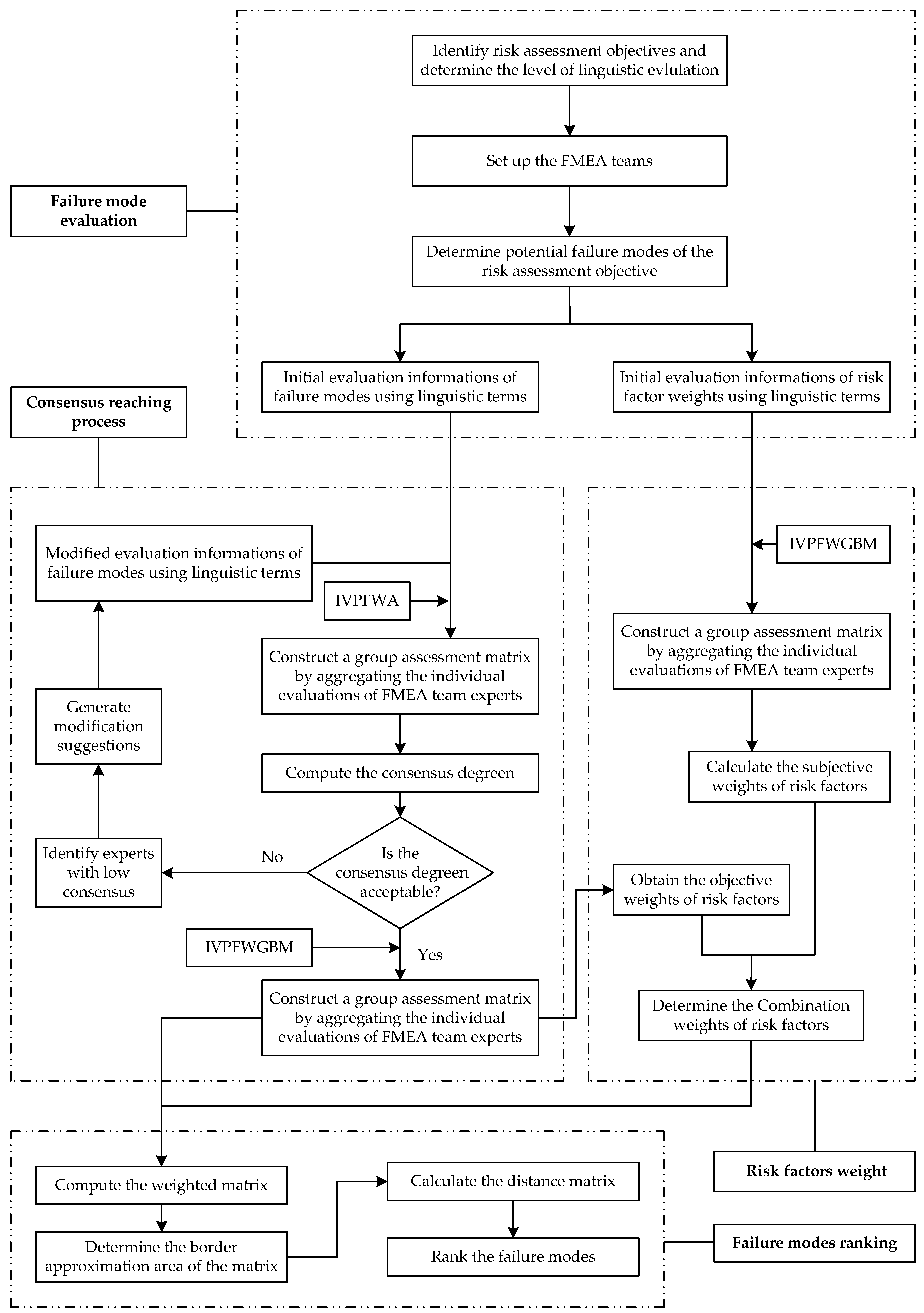
In this section, a method that integrates the IVPFWGBM operator, a consensus-reaching process, and the improved MABAC approach is proposed to rank the failure modes. The flow diagram of the proposed method is shown in Figure 1.

The presented approach consists of four parts: failure mode evaluation, consensus-reaching process, risk factors weight, and failure modes ranking. The relative steps of the proposed method are described as follows.

4.1. Failure Modes Evaluation

Let an FMEA team consist of l cross-functional experts E_k (k = 1, 2, ..., l), which come from various departments and domains, and they are responsible for ranking m potential failure modes FM_i (i = 1, 2, ..., m) and each failure mode is evaluated on n risk factors RF_j (j = 1, 2, ..., n). The weight vector ${\lambda }_k$ (k = 1, 2, ..., l), which satisfies ${\lambda }_k\in [0,1]$ and ${\displaystyle {\sum }_{k=1}^l{\lambda }_k=1}$, is allocated to experts to reflect their relative importance. Let $w_j$ (j=1, 2, ..., n) be the weight vector of risk factors that reflects the relative importance of risk factors, and satisfies $w_j\in [0,1]$ and ${\displaystyle {\sum }_{j=1}^n{w}_j=1}$.

Step 1: Construct linguistic evaluation matrix.

FMEA team experts prefer to employ the linguistic variables in

Table 1. Linguistic terms for rating the weights of risk factors [49].

Linguistic Variables	Abbreviation	IVPFNs
Very high	VH	([0.8000,0.9000],[0.1000,0.2000])
High	H	([0.7000,0.8000],[0.2000,0.3000])
Medium	M	([0.5000,0.6000],[0.4000,0.5000])
Low	L	([0.3000,0.4000],[0.6000,0.7000])
Very low	VL	([0.1000,0.2000],[0.8000,0.9000])

to assess the importance of risk factors, and use the linguistic variables in

Table 2. Linguistic terms for rating the failure modes [49].

LinguisticVariables	Abbreviation	IVPFNs
Extremely high	EH	([0.9000,1.0000],[0.0000,0.1000])
Very high	VH	([0.8000,0.9000],[0.1000,0.2000])
High	H	([0.7000,0.8000],[0.2000,0.3000])
Medium high	MH	([0.6000,0.7000],[0.3000,0.4000])
Medium	M	([0.5000,0.6000],[0.4000,0.5000])
Medium low	ML	([0.4000,0.5000],[0.5000,0.6000])
Low	L	([0.3000,0.4000],[0.6000,0.7000])
Very low	VL	([0.2000,0.3000],[0.7000,0.8000])
Extremely low	EL	([0.1000,0.2000],[0.8000,0.9000])

to evaluate the failure modes’ risk with respect to each risk factor because of the uncertainty and fuzziness of human judgments and the complexity of the assessment objectives. Let the linguistic evaluation matrix of failure modes evaluation provided by E_k be denoted as $L^k={(l_{ij}^k)}_{m\times n}$, and the linguistic assessment matrix of the relative importance of a risk factor given by E_k be denoted as $Z^k={(z_j^k)}_{1\times n}$.

4.2. Consensus-ReachingProcess

To increase the agreement degree of FMEA team experts, a consensus-reaching process is introduced into the risk assessment process of FMEA. According to the evaluation information provided by experts, we will define the consensus degree on four levels, which include the consensus degree on elements of failure modes, the consensus degree on failure modes, the consensus degree on the matrix, and the consensus degree on team experts.

Definition 8.

Let $A^k$ be the assessment matrix provided by the k expert and C be the comprehensive assessment matrix. The consensus degree between assessment matrix $A^k$ and comprehensive assessment matrix C on the element of failure modes FM_i under risk factors RF_j is given as follows:

$$CD{E}_{ij}^k(A^k,C)=\frac{1}{2}(1+grc(a_{ij}^k,c_{ij})),$$

(10)

where $grc(a_{ij}^k,c_{ij})$ is the gray relational coefficient between $a_{ij}^k$ and $c_{ij}$. The $CD{E}_{ij}^k(A^k,C)$ is called the consensus degree on elements of failure modes. Given $A^k$ and C, the elaborated expression of $CD{E}_{ij}^k(A^k,C)$ is

$$CD{E}_{ij}^k(A^k,C)=\frac{1}{2}\left(1+\frac{\min \min \min |s(a_{ij}^k)-s(c_{ij})|+\rho \max \max \max |s(a_{ij}^k)-s(c_{ij})|}{|s(a_{ij}^k)-s(c_{ij})|+\rho \max \max \max |s(a_{ij}^k)-s(c_{ij})|}\right),$$

(11)

where $\rho$ is the identification coefficient, $\rho \in [0,1]$. The smaller the value of the identification coefficient, the larger the range of the gray relational coefficient, but it will not affect the final priority of failure modes [50]. Generally, $\rho =0.5$ [51].

Definition 9.

Let $A^k$ be the assessment matrix provided by the k expert and C be the comprehensive assessment matrix. The consensus degree between assessment matrix $A^k$ and comprehensive assessment matrix C on the failure modes FM_i is defined as:

$$CD{F}_i^k(A^k,C)=\frac{1}{n}{\displaystyle {\sum }_{j=1}^{n}CD{E}_{ij}(A^k,C}),$$

(12)

then $CD{F}_i^k(A^k,C)$ is called the consensus degree on failure modes.

Definition 10.

Let $A^k$ be the assessment matrix provided by the k expert and C be the comprehensive assessment matrix. The consensus degree between assessment matrix $A^k$ and comprehensive assessment matrix C on the matrix $A^k$ is calculated as

$$CD{M}^k(A^k,C)=\frac{1}{mn}{\displaystyle {\sum }_{i=1}^m{\displaystyle {\sum }_{j=1}^{n}CD{E}_{ij}(A^k,C})},$$

(13)

then $CD{M}^k(A^k,C)$ is called the consensus degree on decision-makers.

Definition 11.

Let $A^k$ be the assessment matrix provided by the k expert and C be the comprehensive assessment matrix. The consensus degree on the team experts is determined as

$$CDT(A^k,C)={\displaystyle {\sum }_{k=1}^L{\lambda }_{k}CD{M}^k(A^k,C)}.$$

(14)

Then, we will construct a consensus model.

Step 2: Construct a consensus-reaching process.

Step 2.1: Let $\gamma =1$, $\zeta$ and round, where $\zeta$ and round represents the threshold value and the maximum number of cycles, respectively.

Step 2.2: Convert all linguistic variables in the matrix $L^k$ into the IVPFN according to Table 2 to construct an IVPFN evaluation matrix $A^k={(a_{ij}^k)}_{m\times n}$.

Step 2.3: Construct the comprehensive matrix $C={(c_{ij})}_{m\times n}$ by the internal-valued Pythagorean weighted averaging (IVPFWA) operator [49] to calculate the consensus degree, where

$$\begin{array}{c}{c}_{ij}=IVPFWA(a_{ij}^1,a_{ij}^2,\cdot \cdot \cdot ,a_{ij}^L)\\ =\left(\left[\sqrt{1-{\displaystyle \prod _{k=1}^L{(1-{({\underset{\_}{\mu }}_{P_{ij}}^k)}^2)}^{{\lambda }_k}}},\sqrt{1-{\displaystyle \prod _{k=1}^L{(1-{({\overline{\mu }}_{P_{ij}}^k)}^2)}^{{\lambda }_k}}}\right],\left[{\displaystyle \prod _{k=1}^L{({\underset{\_}{\nu }}_{P_{ij}}^k)}^{{\lambda }_k},{\displaystyle \prod _{k=1}^L{({\overline{\nu }}_{P_{ij}}^k)}^{{\lambda }_k},}}\right]\right).\end{array}$$

(15)

Step 2.4: Compute the consensus degree according to Equations (11)–(14).

Step 2.5: If $CDT(A^k,C)\ge \zeta$ or $\gamma >round$, then go to step 2.8, otherwise go to next step.

Step 2.6: Identify the elements of failure modes for which the consensus degree is lower than the threshold value $\zeta$ by carrying out the follow steps:

(1)

Identify the experts for which the consensus degree is lower than threshold value $\zeta$:

$$ADS=\left\{k\right|CD{M}^k<\zeta \}.$$

(16)

(2)

For the determined experts, the failure modes with $CD{F}_i^k$ lower than $\zeta$ are identified:

$$AFS=\{(k,i)|k\in ADS\cap CD{F}_i^k<\zeta \}.$$

(17)

(3)

Finally, the elements of failure modes that need to be modified are:

$$AES=\{(k,i,j)|(k,i)\in AFS\cap CD{E}_{ij}^k<\zeta \}.$$

(18)

Step 2.7: Generate modification suggestions.

If $(k,i,j)\in AES$, the personalized suggestions for E_k are generated as follows: you are suggested to change your evaluation linguistic term $l_{ij}^k$ for failure modes FM_i under risk factor RF_j to the value ${\widehat{l}}_{ij}^k$, where

$${\widehat{l}}_{ij}^k=\{\begin{array}{l}\mathrm{liguistic}\mathrm{variable}\mathrm{level}\mathrm{minus}\mathrm{one}ifs(a_{ij}^k)\ge s(c_{ij})and{l}_{ij}^k\mathrm{is}\mathrm{not}\mathrm{liguistic}\mathrm{variable}\mathrm{of}\mathrm{the}\mathrm{lowest}\mathrm{level}\\ \mathrm{liguistic}\mathrm{variable}\mathrm{level}\mathrm{plus}\mathrm{one}ifs(a_{ij}^k)<s(c_{ij})and{l}_{ij}^k\mathrm{is}\mathrm{not}\mathrm{liguistic}\mathrm{variable}\mathrm{of}\mathrm{the}\mathrm{highest}\mathrm{level}\end{array},$$

(19)

then let $\gamma =\gamma +1$, go back to step 2.2.

Step 2.8: Output the adjusted IVPFN evaluation matrix.

4.3. Risk Factors Weight

Entropy was developed by Shannon and weaver [52] and is well-suited to reflect the relative importance of the criteria that represent the intrinsic information for assessing issues [14]. Therefore, the entropy method has been used by many researchers for calculating the objective weight of criteria in an MCDM problem [14,36]. In order to reflect the importance of risk factors, we will define an interval-valued Pythagorean fuzzy entropy (IVPFE), which is parallel to interval-valued intuitionistic fuzzy entropy [53], to compute the weight of risk factors.

Definition 12.

Let P be an IVPFS defined in the universe of discourse U. The IVPFE is given as follows:

$$E(P)=\frac{1}{n}{\displaystyle \sum _{i=1}^n\frac{2-\left|{\underset{\_}{\mu }}_{P_i}^2-{\underset{\_}{\nu }}_{P_i}^2\right|-\left|{\overline{\mu }}_{P_i}^2-{\overline{\nu }}_{P_i}^2\right|+{\underset{\_}{\pi }}_{P_i}^2+{\overline{\pi }}_{P_i}^2}{2+\left|{\underset{\_}{\mu }}_{P_i}^2-{\underset{\_}{\nu }}_{P_i}^2\right|+\left|{\overline{\mu }}_{P_i}^2-{\overline{\nu }}_{P_i}^2\right|+{\underset{\_}{\pi }}_{P_i}^2+{\overline{\pi }}_{P_i}^2}}.$$

(20)

Step 3: Aggregate the experts’ preferences into a comprehensive evaluation matrix.

In order to depict the interdependent relationships between experts’ preferences, we can aggregate all individual evaluation information into a collective evaluation matrix $D=(d_{ij})m\times n$ by the IVPFWGBM operator, where $d_{ij}=IVPFWGB{M}_{\lambda }^{x,y}(a_{ij}^1,a_{ij}^2,\cdot \cdot \cdot ,a_{ij}^L)$.

Step 4: Calculate the combination weights of risk factors.

Step4.1: Determine the subjective weights of risk factors.

According to Table 1, we can convert all linguistic variables elements in matrix $Z^k$ into the IVPFN to construct matrix $H^k={(h_j^k)}_{1\times n}$. Subsequently, the IVPFWGBM operator is applied to aggregate all individual valuations for risk factors to construct a collective evaluation matrix $H={(h_j)}_{1\times n}$, where $h_j=IVPFWGB{M}_{\lambda }^{x,y}(h_j^1,h_j^2,\cdot \cdot \cdot ,h_j^L)$.

Then, the normalized subjective weight of each risk factor is computed as follows:

$$w_j^s=\frac{s(h_j)}{{\displaystyle {\sum }_{j=1}^{n}s(h_j)}},(j=1,2,\cdot \cdot \cdot ,n).$$

(21)

Step 4.2: Compute the objective weights of risk factors using the entropy method.

$$E(d_{ij})=\frac{2-\left|{\underset{\_}{\mu }}_{P_{ij}}^2-{\underset{\_}{\nu }}_{P_{ij}}^2\right|-\left|{\overline{\mu }}_{P_{ij}}^2-{\overline{\nu }}_{P_{ij}}^2\right|+{\underset{\_}{\pi }}_{P_{ij}}^2+{\overline{\pi }}_{P_{ij}}^2}{2+\left|{\underset{\_}{\mu }}_{P_{ij}}^2-{\underset{\_}{\nu }}_{P_{ij}}^2\right|+\left|{\overline{\mu }}_{P_{ij}}^2-{\overline{\nu }}_{P_{ij}}^2\right|+{\underset{\_}{\pi }}_{P_{ij}}^2+{\overline{\pi }}_{P_{ij}}^2},(i=1,2,\cdot \cdot \cdot ,m;j=1,2,\cdot \cdot \cdot ,n).$$

(22)

Then, the normalized objective weight of each risk factor can be calculated by applying the following formula.

$$w_j^o=\frac{{\displaystyle {\sum }_{i=1}^m(1-E(d_{ij}))}}{{\displaystyle {\sum }_{j=1}^n{\displaystyle {\sum }_{i=1}^m(1-E(d_{ij}))}}},(i=1,2,\cdot \cdot \cdot ,m;j=1,2,\cdot \cdot \cdot ,n).$$

(23)

Step 4.3: Obtain the integration weights of risk factors:

$$w_j=\sigma w_j^s+(1-\sigma )w_j^o,(i=1,2,\cdot \cdot \cdot ,m;j=1,2,\cdot \cdot \cdot ,n),$$

(24)

where parameter $\sigma$ is the relative importance coefficient of the subjective weight and satisfies $0\le \sigma \le 1$. Generally, the subjective weight and objective weight are assumed to be equally important, namely, $\sigma =0.5$.

4.4. Failure Modes Ranking

As a particularly pragmatic and reliable tool, the MABAC approach is applied to solve MCDM problems because it can obtain a stable solution. However, this method fails to capture the interdependence between failure modes. Therefore, an improved MABAC method is utilized to determine the ranking order of failure modes in which the border approximation area is calculated by the IVPFGBM operator instead of the geometry mean operator.

Step 5: Compute the weighted group decision matrix Y.

The weighted decision matrix $Y={(y_{ij})}_{m\times n}$ can be determined by the following formula:

$$y_{ij}=w_j{d}_{ij}=\left(\left[\sqrt{1-{(1-{\underset{\_}{\mu }}_{P_{ij}}^2)}^{w_j}},\sqrt{1-{(1-{\overline{\mu }}_{P_{ij}}^2)}^{w_j}}\right],\left[{({\underset{\_}{\nu }}_{P_{ij}})}^{w_j},{({\overline{\nu }}_{P_{ij}})}^{w_j}\right]\right),$$

(25)

where $y_{ij}$ is a weighted IVPFN and $d_{ij}$ are the elements of the collective evaluation matrix D.

Step 6: Determine the border approximation area vector G.

The border approximation area for each risk factor is computed by applying the IVPFGBM operator as:

$$g_j=IVPFGBM(y_{1j},y_{2j},\cdot \cdot \cdot ,y_{mj})=([{\underset{\_}{\mu }}_{P_j},{\overline{\mu }}_{P_j}],[{\underset{\_}{\nu }}_{P_j},{\overline{\nu }}_{P_j}]).$$

(26)

Then, the border approximation area vector G can be constructed in the following format $G=\left(g_1,g_2,\cdot \cdot \cdot ,g_n\right)$.

Step 7: Construct the distance matrix X.

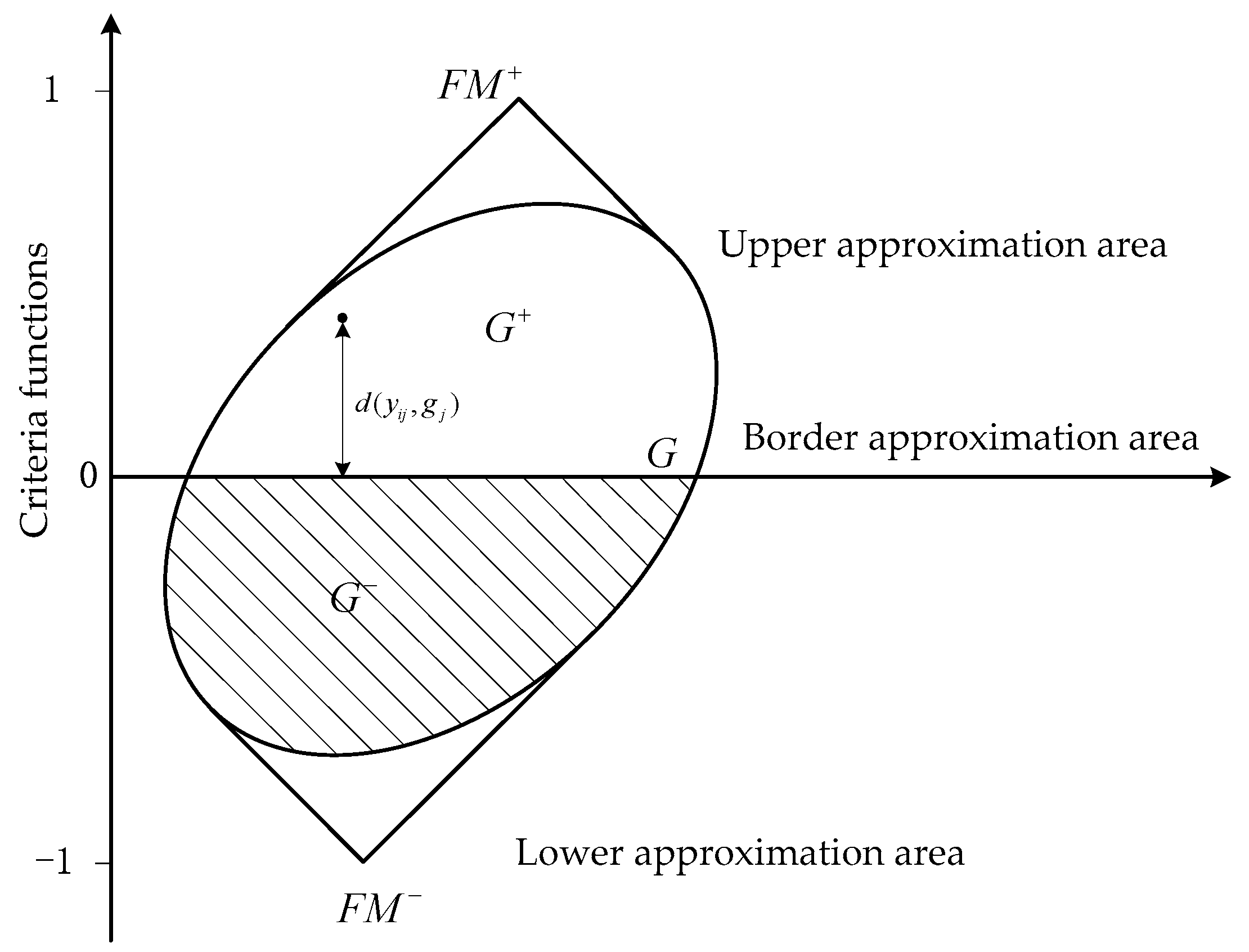
The distance of the failure modes from the border approximation area (See Figure 2) is calculated by Equation (2) to construct the distance matrix $X={(x_{ij})}_{m\times n}$, where

$$x_{ij}=\{\begin{array}{ll}d(y_{ij},g_j)& ifs\left(y_{ij}\right)\ge s\left(g_j\right)\\ -d(y_{ij},g_j)& ifs\left(y_{ij}\right)<s\left(g_j\right)\end{array}.$$

(27)

Step 8: Determine the ranking of failure modes.

All failure modes will be included in approximation areas that consist of an upper approximation area $G^{+}$, a border approximation area $G$, and a lower approximation area $G^{-}$. The ideal failure mode (FM⁺) is located in the upper approximation area, while the anti-ideal failure mode (FM⁻) is located in the lower approximation area (See Figure 2). Consequently, in order to select the ideal failure mode, it is necessary to have as many risk factors as possible belonging to the upper approximation area. We can obtain the closeness coefficient ${\theta }_i$ for each failure mode by computing the sum of the row elements of the distance matrix X.

$${\theta }_i={\displaystyle {\sum }_{j=1}^n{x}_{ij}},i=1,2,\cdot \cdot \cdot ,m.$$

(28)

The risk priority of failure modes is obtained according to the decreasing order of the closeness coefficient.

5. Case Study

In this section, the development of new product—a horizontal directional drilling (HDD) machine [17,54]—is selected as an illustrative example to demonstrate the applicability of the proposed method. As an important piece of equipment in trenchless construction, the HDD machine is a particularly complex product that contains multiple sub-systems, such as an engine system, a hydraulic system, and an electric system. The conceptual model of the HDD machine is shown in Figure 3.

In what follows, we use the proposed approach to identify the key failure modes in the product development of the HDD machine. The steps are summarized as follows.

5.1. Implement the Proposed Method

An FMEA team consisting of five cross-functional experts E_k (k = 1,2,3,4,5) from different departments is formed to identify the most important failure modes; we suppose that the relative weights of the five team experts are assigned as 0.15, 0.2, 0.25, 0.1, and 0.3 according to their different professional knowledge and expertise. The FMEA team identifies nine potential failure modes through brainstorming, namely, gear abrasion of dynamic head, action invalidation of force motor, non-normal friction of pedrail, leak of hydraulic system, abrasion of feed mechanism, unexpected halt of engine, cavitation erosion of hydraulic pump, failures of hydraulic system induced by hydraulic oil pollution, and nozzle choking of aiguilles.

Step1: Construct linguistic assessment matrix.

In a practical application, the five experts use the linguistic variables to evaluate the nine failure modes on each risk factor and the relative importance of risk factors; the evaluation results are shown in

Table 3. Evaluation information on the nine failure modes provided by the FMEA team experts.

Failure Modes	Severity(S)					Occurrence(O)					Detection(D)
	E1	E2	E3	E4	E5	E1	E2	E3	E4	E5	E1	E2	E3	E4	E5
FM1	ML	MH	ML	M	M	M	M	M	MH	M	M	L	ML	ML	ML
FM2	MH	MH	H	M	H	M	MH	H	MH	MH	MH	MH	ML	MH	M
FM3	MH	M	H	MH	M	ML	ML	L	M	M	H	H	H	MH	MH
FM4	M	MH	ML	M	M	L	M	L	M	M	VL	ML	VL	L	VL
FM5	M	H	MH	MH	M	M	ML	M	M	M	L	ML	VL	L	VL
FM6	H	H	MH	MH	H	H	MH	M	MH	M	L	M	L	EL	L
FM7	MH	MH	H	MH	MH	VH	MH	VH	MH	H	MH	M	MH	M	M
FM8	EH	H	EH	H	VH	ML	M	L	ML	ML	ML	ML	L	L	L
FM9	ML	M	ML	ML	M	M	M	ML	M	M	M	M	M	ML	ML
Factor weight	H	VH	H	VH	H	H	M	H	M	M	VL	L	L	M	L

.

Step 2: Construct a consensus-reaching process.

Step 2.1: Generally, the threshold value and the maximum number of cycles are determined by the team experts according to the actual situation. In this case study, let $\gamma =1$, $\zeta =0.86$, and $round=3$.

Step 2.2: Convert all linguistic variables in each linguistic evaluation matrix L¹, L², L³, L⁴, and L⁵ into the IVPFNs according to Table 2 to construct assessment matrices A¹, A², A³, A⁴, and A⁵.

Step 2.3: The collective matrix C is aggregated by the IVPFWA operator to compute the consensus degree.

$$C=\left(\begin{array}{c}([0.4896,0.5092],[0.4129,0.5144])\\ ([0.6528,0.7545],[0.2470,0.3492])\\ ([0.5877,0.6902],[0.3130,0.4162])\\ ([0.5025,0.6031],[0.3933,0.5005])\\ ([0.5858,0.6879],[0.3149,0.4175])\\ ([0.6692,0.7703],[0.2305,0.3318])\\ ([0.6287,0.7297],[0.2711,0.3722])\\ ([0.8310,1.0000],[0.0000,0.1712])\\ ([0.4542,0.5542],[0.4472,0.5477])\end{array}\begin{array}{c}([0.5117,0.6119],[0.3887,0.4890])\\ ([0.6171,0.7186],[0.2830,0.3849])\\ ([0.4254,0.5252],[0.4786,0.5797])\\ ([0.4355,0.5352],[0.4704,0.5720])\\ ([0.4825,0.5826],[0.4183,0.5186])\\ ([0.5701,0.6720],[0.3307,0.4331])\\ ([0.7246,0.8310],[0.1712,0.2781])\\ ([0.4028,0.5025],[0.5005,0.6012])\\ ([0.4780,0.5780],[0.4229,0.5233])\end{array}\begin{array}{c}([0.4010,0.5008],[0.5015,0.6021])\\ ([0.5307,0.6315],[0.3716,0.4733])\\ ([0.6645,0.7656],[0.2352,0.3366])\\ ([0.2651,0.3626],[0.6444,0.7453])\\ ([0.2788,0.3767],[0.6297,0.7305])\\ ([0.3422,0.4402],[0.5694,0.6711])\\ ([0.5442,0.6446],[0.3656,0.4573])\\ ([0.3393,0.4389],[0.5629,0.6632])\\ ([0.4639,0.5640],[0.4373,0.5378])\end{array}\right)$$

Step 2.4: Calculate the consensus degree.

Based on Equations (11) and (12), the CDF value is determined as follows.

$$CDF=\left(\begin{array}{ccccc}0.8381& 0.8288& 0.9147& 0.9143& 0.9715\\ 0.8035& 0.8659& 0.7972& 0.8232& 0.8994\\ 0.9204& 0.8646& 0.7959& 0.8604& 0.8046\\ 0.8562& 0.7725& 0.7806& 0.8943& 0.8834\\ 0.8775& 0.7633& 0.8981& 0.9301& 0.8455\\ 0.8420& 0.8354& 0.8397& 0.7942& 0.8675\\ 0.8508& 0.8364& 0.8207& 0.8364& 0.8921\\ 0.9051& 0.7694& 0.8459& 0.8626& 0.9007\\ 0.8830& 0.8877& 0.8433& 0.8644& 0.8690\end{array}\right).$$

Then, according to Equation (13), the CDM value is calculated as follows.

$$CDM=(0.8641,0.8249,0.8374,0.8644,0.8815).$$

Finally, using Equation (14), the CDT value is obtained as $CDT=0.8548$.

Step 2.5: Due to $CDT<\zeta$, go to next step.

Step 2.6: Based on Equations (16)–(18), the elements of failure modes that need to be modified are determined to be:

AES = {(2,1,1), (2,1,3), (2,4,1), (2,4,2), (2,4,3), (2,5,1), (2,5,2), (2,5,3), (2,6,3), (2,7,2), (2,8,1), (2,8,2), (2,8,3), (3,2,2), (3,2,3), (3,3,1), (3,3,2), (3,4,1), (3,4,2), (3,4,3), (3,6,1), (3,6,2), (3,7,1), (3,7,2), (3,7,3), (3,8,2), (3,9,1), (3,9,2)}.

Step 2.7: According to Equation (19), the personalized suggestions for experts are obtained. The modified assessment information on the nine failure modes is shown in

Table 4. Assessment information on the nine failure modes by FMEA team experts.

Failure Modes	Severity(S)					Occurrence(O)					Detection(D)
	E1	E2	E3	E4	E5	E1	E2	E3	E4	E5	E1	E2	E3	E4	E5
FM1	ML	M	ML	M	M	M	M	M	MH	M	M	ML	ML	ML	ML
FM2	MH	MH	H	M	H	M	MH	MH	MH	MH	MH	MH	M	MH	M
FM3	MH	M	MH	MH	M	ML	ML	ML	M	M	H	H	H	MH	MH
FM4	M	M	M	M	M	L	ML	ML	M	M	VL	L	L	L	VL
FM5	M	MH	MH	MH	M	M	M	M	M	M	L	L	VL	L	VL
FM6	H	H	H	MH	H	H	MH	MH	MH	M	L	ML	L	EL	L
FM7	MH	MH	MH	MH	MH	VH	H	H	MH	H	MH	M	M	M	M
FM8	EH	VH	EH	H	VH	ML	ML	ML	ML	ML	ML	L	L	L	L
FM9	ML	M	M	ML	M	M	M	M	M	M	M	M	M	ML	ML

. Then, let $\gamma =2$, go back to step 2.2.

Next is the second round of the consensus-reaching process.

Step 2.2: Convert all linguistic variables in each linguistic evaluation matrix L² and L³ into the IVPFNs according to Table 2 to construct assessment matrices A² and A³.

Step 2.3: Based on the IVPFWA operator, the comprehensive matrix C is obtained as follows:

$$C=\left(\begin{array}{c}([0.4639,0.5640],[0.4373,0.5378])\\ ([0.6528,0.7545],[0.2470,0.3492])\\ ([0.5542,0.6547],[0.3464,0.4472])\\ ([0.5000,0.6000],[0.4000,0.5000])\\ ([0.5592,0.6596],[0.3415,0.4423])\\ ([0.6916,0.7920],[0.2083,0.3088])\\ ([0.6000,0.7000],[0.3000,0.4000])\\ ([0.8434,1.0000],[0.0000,0.1578])\\ ([0.4780,0.5780],[0.4229,0.5233])\end{array}\begin{array}{c}([0.5117,0.6119],[0.3887,0.4890])\\ ([0.5870,0.6873],[0.3132,0.4136])\\ ([0.4441,0.5442],[0.4573,0.5578])\\ ([0.4330,0.5329],[0.4700,0.5708])\\ ([0.5000,0.6000],[0.4000,0.5000])\\ ([0.5927,0.6941],[0.3077,0.4096])\\ ([0.7105,0.8132],[0.1877,0.2905])\\ ([0.4000,0.5000],[0.5000,0.6000])\\ ([0.5000,0.6000],[0.4000,0.5000])\end{array}\begin{array}{c}([0.4173,0.5173],[0.4835,0.5838])\\ ([0.5492,0.6497],[0.3514,0.4522])\\ ([0.6645,0.7656],[0.2352,0.3366])\\ ([0.2604,0.3594],[0.6431,0.7434])\\ ([0.2507,0.3496],[0.6531,0.7533])\\ ([0.3112,0.4096],[0.5954,0.6960])\\ ([0.5173,0.6176],[0.3831,0.4835])\\ ([0.3176,0.4173],[0.5838,0.6840])\\ ([0.4639,0.5640],[0.4373,0.5378])\end{array}\right)$$

Step 2.4 Compute the consensus degree.

Based on Equations (11) and (12), the CDF value is determined as follows.

$$CDF=\left(\begin{array}{ccccc}0.8456& 0.9162& 0.8967& 0.8560& 0.8919\\ 0.8120& 0.8695& 0.8756& 0.8266& 0.8860\\ 0.8570& 0.8511& 0.8570& 0.8252& 0.8193\\ 0.8469& 0.9129& 0.9129& 0.8849& 0.8428\\ 0.8834& 0.8965& 0.8998& 0.8965& 0.8238\\ 0.8929& 0.8973& 0.9668& 0.7994& 0.8608\\ 0.8489& 0.9594& 0.9594& 0.8897& 0.8989\\ 0.8896& 0.9087& 0.9410& 0.8729& 0.8401\\ 0.8847& 0.9042& 0.9263& 0.8653& 0.8917\end{array}\right).$$

Then, according to Equation (13), the CDM value is calculated as follows.

$$CDM=(0.8623,0.9042,0.9150,0.8574,0.8939).$$

Finally, using Equation (14), the CDT value is obtained as $CDT=0.8929$.

Step 2.5: Due to $CDT>\zeta$, go to step 2.8.

Step 2.8: Output the adjusted IVPFN assessment matrix.

Step 3: The comprehensive evaluation matrix D is obtained by considering the weights of experts and applying the IVPFWGBM operator. The result is as follows.

$$D=\left(\begin{array}{c}([0.8594,0.8928],[0.2048,0.2573])\\ ([0.9154,0.9422],[0.1199,0.1669])\\ ([0.8912,0.9203],[0.1591,0.2082])\\ ([0.8740,0.9052],[0.1835,0.2343])\\ ([0.8923,0.9213],[0.1571,0.2061])\\ ([0.9293,0.9543],[0.0956,0.1418])\\ ([0.9052,0.9327],[0.1356,0.1835])\\ ([0.9640,0.9867],[0.0403,0.0801])\\ ([0.8629,0.8960],[0.1988,0.2509])\end{array}\begin{array}{c}([0.8781,0.9088],[0.1784,0.2287])\\ ([0.9000,0.9281],[0.1441,0.1925])\\ ([0.8517,0.8863],[0.2153,0.2687])\\ ([0.8441,0.8802],[0.2255,0.2802])\\ ([0.8740,0.9052],[0.1835,0.2343])\\ ([0.9028,0.9305],[0.1421,0.1901])\\ ([0.9337,0.9583],[0.0898,0.1353])\\ ([0.8374,0.8740],[0.2343,0.2894])\\ ([0.8740,0.9052],[0.1835,0.2343])\end{array}\begin{array}{c}([0.8441,0.8796],[0.2264,0.2806])\\ ([0.8904,0.9195],[0.1608,0.2100])\\ ([0.9226,0.9483],[0.1081,0.1547])\\ ([0.7693,0.8192],[0.3166,0.3836])\\ ([0.7667,0.8169],[0.3210,0.3885])\\ ([0.7822,0.8318],[0.2980,0.3650])\\ ([0.8796,0.9101],[0.1762,0.2264])\\ ([0.8011,0.8441],[0.2806,0.3413])\\ ([0.8606,0.8937],[0.2037,0.2560])\end{array}\right).$$

Step 4: Calculate the combination weights of risk factors.

Step 4.1: Determine the subjective weights of risk factors.

The collective evaluation matrix H of risk factors is constructed by aggregating all individual assessments for risk factors. Subsequently, the normalized subjective weights of risk factors based on Equation (21) are determined to be $w_j^s={(0.4021,0.3602,0.2378)}^{\mathrm{T}}$.

Step 4.2: Compute the objective weights of risk factors by the entropy method.

Based on the comprehensive evaluation matrix D, the entropy value of each failure mode with regard to each risk factor can be calculated by applying Equation (22). Then, the objective weights for each risk factor can be derived as $w_j^o={(0.3568,0.3390,0.3042)}^{\mathrm{T}}$ by utilizing Equation (23).

Step 4.3: Obtain the combination weights of risk factors.

Based on the subjective weights and objective weights of risk factors, the combination weights of risk factors are calculated as $w_j={(0.3795,0.3496,0.2709)}^{\mathrm{T}}$ according to Equation (24).

Step 5: Compute the weighted group decision matrix Y.

The weighted decision matrix can be calculated by Equation (25) as follows.

$$Y=\left(\begin{array}{c}([0.6317,0.6739],[0.5479,0.5974])\\ ([0.7062,0.7509],[0.4471,0.5069])\\ ([0.6717,0.7138],[0.4978,0.5513])\\ ([0.6494,0.6912],[0.5255,0.5765])\\ ([0.6732,0.7154],[0.4954,0.5492])\\ ([0.7284,0.7748],[0.4102,0.4765])\\ ([0.6912,0.7340],[0.4684,0.5255])\\ ([0.7964,0.8648],[0.2957,0.3837])\\ ([0.6359,0.6782],[0.5416,0.5917])\end{array}\begin{array}{c}([0.6346,0.6762],[0.5474,0.5970])\\ ([0.6636,0.7063],[0.5080,0.5621])\\ ([0.6030,0.6541],[0.5846,0.6317])\\ ([0.5944,0.6373],[0.5941,0.6409])\\ ([0.6295,0.6711],[0.5528,0.6021])\\ ([0.6676,0.7103],[0.5055,0.5597])\\ ([0.7157,0.7638],[0.4306,0.4969])\\ ([0.5870,0.6295],[0.6021,0.6482])\\ ([0.6295,0.6711],[0.5528,0.6021])\end{array}\begin{array}{c}([0.5353,0.5757],[0.6687,0.7088])\\ ([0.5892,0.6301],[0.6095,0.6552])\\ ([0.6349,0.6804],[0.5473,0.6032])\\ ([0.4643,0.5100],[0.7323,0.7714])\\ ([0.4620,0.5078],[0.7350,0.7740])\\ ([0.4756,0.5225],[0.7204,0.7611])\\ ([0.5757,0.6161],[0.6248,0.6687])\\ ([0.4927,0.5353],[0.7088,0.7473])\\ ([0.5533,0.5935],[0.6498,0.6914])\end{array}\right)$$

Step 6: Determine the border approximation area vector G.

According to Equation (26), the border approximation area vector G can be obtained as

$$G=(([0.6881,0.7345],[0.4752,0.5323]),([0.6367,0.6796],[0.5442,0.5951]),([0.5323,0.5757],[0.6696,0.7120])).$$

Step7: Construct the distance matrix X.

The distance of failure modes from the border approximation area is computed by Equation (27); the distance matrix is determined as

$$X=\left(\begin{array}{ccc}-0.0799& -0.0041& 0.0038\\ 0.0261& 0.0382& 0.0772\\ -0.0261& -0.0456& 0.1459\\ -0.0567& -0.0567& -0.0880\\ -0.0240& -0.0105& -0.0920\\ 0.0591& 0.0416& -0.0715\\ 0.0071& 0.1161& 0.0589\\ 0.1846& -0.0662& -0.0528\\ -0.0743& -0.0105& 0.0275\end{array}\right)$$

Step 8: Determine the ranking of failure modes.

The closeness coefficient ${\theta }_i$ can be calculated by Equation (28) as follows.

$$\theta =(\begin{array}{ccccccccc}-0.0801& 0.1415& 0.0742& -0.2014& -0.1266& 0.0293& 0.1821& 0.0657& -0.0573\end{array})$$

The risk priority of failure modes is ranked as FM₇ > FM₂ > FM₃ > FM₈ > FM₆ > FM₉ > FM₁ > FM₅ > FM₄ by the decreasing order of the closeness coefficient ${\theta }_i$.

5.2. Sensitivity Analysis

In the above case study, we set the consensus threshold value $\zeta =0.86$ in the application of the consensus-reaching process. Generally, the consensus threshold value plays an important role in the consensus-reaching process. Hence, a sensitivity analysis by setting different $\zeta$ values is performed to validate the performance of the ranking order of failure modes. The relative results are shown in

Table 5. Ranking of different threshold values $\zeta$.

Failure Modes	$\mathit{\zeta }=0.84$		$\mathit{\zeta }=0.86$		$\mathit{\zeta }=0.88$		$\mathit{\zeta }=0.90$
	Scores	Ranking	Scores	Ranking	Scores	Ranking	Scores	Ranking
FM1	−0.0604	6	−0.0801	7	−0.0723	7	−0.0544	6
FM2	0.1437	2	0.1415	2	0.1276	2	−0.1181	2
FM3	0.0782	3	0.0742	3	0.0744	4	0.0622	3
FM4	−0.2074	9	−0.2014	9	−0.1944	9	−0.1995	9
FM5	−0.1129	8	−0.1266	8	−0.1304	8	−0.0853	7
FM6	0.0106	5	0.0293	5	0.0422	5	0.0375	5
FM7	0.2140	1	0.1821	1	0.1781	1	0.1900	1
FM8	0.0563	4	0.0657	4	0.0856	3	0.0618	4
FM9	−0.0800	7	−0.0573	6	−0.0570	6	−0.0989	8
n(E)	0		2		4		5
n(FM)	0		13		27		38

n(E) is the number of modified expert evaluations, and n(FM) is the number of modified failure modes.

.

From Table 5, it can be observed that the scores of the nine failure modes have changed under the different values of $\zeta$. The ranking order of some failure modes is not the same, but the FM₂, FM₄, FM₆, and FM₇ failure modes have the same ranking. In addition, the values of n(E) and n(FM) increase with an increasing $\zeta$, which illustrates that there are more evaluation values that need to be modified in the first round when the value of $\zeta$ is increasing. The above analysis indicates that the value of $\zeta$ has a great influence on the ranking of failure modes and the numbers of modifications. Therefore, in a real application, determining a suitable value of $\zeta$ is of significance and benefit to obtain a suitable ranking of failure modes and simplify the proposed method.

5.3. Comparisons and Discussion

To further demonstrate the effectiveness of the proposed method, we use the result to compare some similar approaches, including the RPN method, the fuzzy TOPSIS [14], the fuzzy VIKOR [36], the fuzzy MULTIMOOR [20], and the IFHWED-based FMEA [54] in this section.

Table 6. Ranking of failure modes of different approaches.

Failure Modes	RPN Method					Proposed Method		[14]	[36]	[20]	[54]
	S	O	D	RPN	Ranking	Round 1	Round 2
FM1	6	6	5	180	7	6	7	6	7	7	7
FM2	8	7	6	336	1	2	2	3	2	3	2
FM3	7	5	8	280	3	3	3	4	5	4	5
FM4	6	5	4	120	9	9	9	9	8	9	9
FM5	7	6	4	168	8	8	8	7	6	6	6
FM6	8	7	4	224	4	5	5	5	3	5	4
FM7	7	8	6	336	1	1	1	2	1	2	1
FM8	10	5	4	200	6	4	4	1	4	1	3
FM9	6	6	6	216	5	7	6	8	9	8	8

The crisp values of S, O, and D are obtained by transforming the elements of matrix C (Step2.3) by the equation $c(c_{ij})=ceil(10\times (s(c_{ij})+1)/2)$, where $ceil(x)$ is a function that returns the smallest integer $\ge x$. RPN: risk priority number.

shows the ranking results of all nine failure modes obtained by implementing the six approaches.

The ranking order of failure modes obtained by the proposed method is partly different from the ones according to the RPN value, but FM₇ possesses the highest risk in the two methods. The FM₂ and FM₇ failure modes have the same risk in the RPN method, which indicates that different values of S, O, and D may produce the same value of RPN. In this situation, it is difficult to distinguish the risk between FM₂ and FM₇ for a decision-maker. However, the risk of FM₂ is lower than that of FM₇ in the proposed method. Therefore, this drawback of the RPN approach can be solved easily by using the proposed method.

The priority of the nine failure modes produced by the fuzzy TOPSIS method is significantly different from the ones determined by the proposed approach. The ranking order obtained by the fuzzy TOPSIS method may be irrational because it does not take into account the interdependent relationships between the experts’ preferences. However, the process of risk assessment based on the FMEA team is considered as a group decision process, and there are many different types of correlations between experts. In addition, each FMEA team expert was considered to have equal importance in the fuzzy TOPSIS method. In reality, FMEA team experts usually come from various departments, and have different professional backgrounds, practical experiences, and knowledge structures. Therefore, they should be assigned different importance during risk assessments.

We can see that there are some differences between the priority of failure modes determined by the proposed method and the fuzzy VIKOR approach. The ranking results determined by the fuzzy VIKOR method may be unreasonable because the consensus-reaching process and the experts’ judgments dependencies were not considered in the risk assessment. For example, FM₉ was the least important failure mode using the fuzzy VIKOR method, whereas it ranked sixth using the proposed method. Interestingly, FM₆ ranked before FM₃ with the fuzzy VIKOR approach, however, the latter is more important in reality. Therefore, FM₃ was merited a higher priority in comparison with FM₆ in our proposed method. Furthermore, the solution obtained through the fuzzy VIKOR method compared with the proposed approach is a set of compromise solutions.

Apart from FM₁, FM₄, and FM₆, the ranking orders of the failure modes obtained by the fuzzy MULTIMOORA approach are totally different from those determined through the proposed method. These inconsistent ranking results may be expressed by the fact that the subjective weights of risk factors were not taken into account in the fuzzy MULTIMOORA method, which may result in irrational rankings of failure modes. For example, FM₈ is given to be a more important failure mode than FM₇ according to the fuzzy MULTIMOORA approach. However, in the proposed approach, it ranks only the fourth position; FM₇ has the top risk priority, which also can be validated by the IFHWED-based and the fuzzy VIKOR methods. In addition, the consensus-reaching process is not considered in the fuzzy MULTIMOORA approach, which may be another reason that leads to the biased ranking results.

As shown in Table 5, the failure modes for FM₃, FM₅, FM₆, FM₈, and FM₉ have different ranking orders between the proposed approach and IFHWED-based method. Interestingly, the sorting positions of FM₅ and FM₉ have been interchanged in the proposed method comparing with the IFHWED-based approach. There are many different types of interdependent relationships between the experts’ preferences in the real world because of the mutual influences of FMEA team experts. However, the interdependent relationships among experts’ preferences are not considered in the IFHWED-based method, which may be the reason that results in the different ranking results. In addition, the IFHWED-based approach also fails to take into account the consensus-reaching process.

Through the comparative analysis above, we can conclude that the risk evaluation results determined by the proposed approach are more reasonable and accurate than those obtained by the fuzzy TOPSIS, fuzzy VIKOR, fuzzy MULTIMOORA, and IFHWED-based methods. Compared with the listed approaches, the advantages of the proposed method are summarized as follows:

(1)

The IVPFWGBM operator was used to aggregate the experts’ preferences into group assessments, which sufficiently reflect the interdependent relationships between the experts’ preferences.

(2)

Compared with the other improved FMEA approach, the ranking results obtained by the proposed method are more acceptable because the level of agreement between decision-maker and group is considered through introducing a consensus-reaching process into the risk assessment process of FMEA.

(3)

The ranking results of failure modes obtained by the proposed approach are more reasonable when compared with the other improved FMEA methods; the reason is that the improved MABAC method adopted the IVPFGBM operator to construct the border approximation area matrix, which considers the direct and indirect relationships among failure modes.

6. Conclusions

In this paper, a new FMEA method based on a consensus reaching process, the IVPFWGBM operator, and a modified MABAC approach was developed to obtain the risk priority of failure modes under an interval-valued Pythagorean fuzzy environment. In the proposed method, all assessment information of failure modes with respect to risk factors was provided by the FMEA team experts in the form of linguistic variables expressed by the IVPFNs. Then, the consensus-reaching process was applied to achieve an acceptable level of consensus before aggregating the evaluation information of FMEA team experts. Subsequently, the group decision matrix was constructed by aggregating the experts’ preferences information using the IVPFWGBM operator. Finally, the improved MABAC approach was used to rank the risk priority of failure modes. In addition, the effectiveness and feasibility of the proposed approach was demonstrated with its application to the development of a new product, namely, a horizontal directional drilling machine; the risk priority of failure modes obtained by the proposed method is more reasonable, reliable, and practical than those produced by other improved FMEA approaches.

Inevitably, there are some limitations to the proposed approach. The proposed approach does not consider the psychological behavior of the FMEA team experts and also neglects the correlations between risk factors, both of which may result in unreasonable ranking results. Hence, in further research, the following directions deserve to be focused on. Firstly, an analytic network process can be introduced into the developed method to reflect the interdependent relationships between risk factors. Secondly, extending the proposed approach by considering the psychological behavior of the experts in the risk evaluation process is recommended. In addition, the method proposed in the paper can be utilized for other engineering fields.

References

- Stamatis, D.H. Failure Mode and Effect Analysis: Fmea from Theory to Execution; ASQ Quality Press: Milwaukee, WI, USA, 2003; p. 80. [Google Scholar]
- Liu, H.-C.; Liu, L.; Liu, N. Risk evaluation approaches in failure mode and effects analysis: A literature review. Expert Syst. Appl. 2013, 40, 828–838. [Google Scholar] [CrossRef]
- Du, Y.; Mo, H.; Deng, X.; Sadiq, R.; Deng, Y. A new method in failure mode and effects analysis based on evidential reasoning. Int. J. Syst. Assur. Eng. Manag. 2014, 5, 1–10. [Google Scholar] [CrossRef]
- Bowles, J.B.; Pelaez, C.E. Fuzzy logic prioritization of failures in a system failure mode, effects and criticality analysis. Reliab. Eng. Syst. Saf. 1995, 50, 203–213. [Google Scholar] [CrossRef]
- Jiang, W.; Xie, C.; Wei, B.; Zhou, D. A modified method for risk evaluation in failure modes and effects analysis of aircraft turbine rotor blades. Adv. Mech. Eng. 2016, 8. [Google Scholar] [CrossRef]
- Tazi, N.; Châtelet, E.; Bouzidi, Y. Using a hybrid cost-FMEA analysis for wind turbine reliability analysis. Energies 2017, 10, 276. [Google Scholar] [CrossRef]
- Liu, H.; Deng, X.; Jiang, W. Risk evaluation in failure mode and effects analysis using fuzzy measure and fuzzy integral. Symmetry 2017, 9, 162. [Google Scholar] [CrossRef]
- Nguyen, T.L.; Shu, M.H.; Hsu, B.M. Extended FMEA for sustainable manufacturing: An empirical study in the non-woven fabrics industry. Sustainability 2016, 8, 939. [Google Scholar] [CrossRef]
- Xia, M.; Xu, Z.; Zhu, B. Geometric Bonferroni means with their application in multi-criteria decision making. Knowl. Based Syst. 2013, 40, 88–100. [Google Scholar] [CrossRef]
- Guo, J. A risk assessment approach for failure mode and effects analysis based on intuitionistic fuzzy sets and evidence theory. J. Intell. Fuzzy Syst. 2016, 30, 869–881. [Google Scholar] [CrossRef]
- Herrera, F.; Herrera-Viedma, E.; Verdegay, J.L. A model of consensus in group decision making under linguistic assessments. Fuzzy Sets Syst. 1996, 78, 73–87. [Google Scholar] [CrossRef]
- Herrera-Viedma, E.; Herrera, F.; Chiclana, F. A consensus model for multiperson decision making with different preference structures. IEEE Trans. Syst. Man Cybern. Part A Syst. Hum. 2002, 32, 394–402. [Google Scholar] [CrossRef]
- Wang, X.; Zhang, Y.; Shen, G. An improved FMECA for feed system of CNC machining center based on ICR and DEMATEL method. Int. J. Adv. Manuf. Technol. 2016, 83, 43–54. [Google Scholar] [CrossRef]
- Song, W.; Ming, X.; Wu, Z.; Zhu, B. Failure modes and effects analysis using integrated weight-based fuzzy TOPSIS. Int. J. Comput. Integr. Manuf. 2013, 26, 1172–1186. [Google Scholar] [CrossRef]
- Bozdag, E.; Asan, U.; Soyer, A.; Serdarasan, S. Risk prioritization in failure mode and effects analysis using interval type-2 fuzzy sets. Expert Syst. Appl. 2015, 42, 4000–4015. [Google Scholar] [CrossRef]
- Mohsen, O.; Fereshteh, N. An extended VIKOR method based on entropy measure for the failure modes risk assessment—A case study of the geothermal power plant (GPP). Saf. Sci. 2017, 92, 160–172. [Google Scholar] [CrossRef]
- Zhang, Z.; Chu, X. Risk prioritization in failure mode and effects analysis under uncertainty. Expert Syst. Appl. 2011, 38, 206–214. [Google Scholar] [CrossRef]
- Kutlu, A.C.; Ekmekçioğlu, M. Fuzzy failure modes and effects analysis by using fuzzy TOPSIS-based fuzzy ahp. Expert Syst. Appl. 2012, 39, 61–67. [Google Scholar] [CrossRef]
- Chai, K.C.; Jong, C.H.; Tay, K.M.; Lim, C.P. A perceptual computing-based method to prioritize failure modes in failure mode and effect analysis and its application to edible bird nest farming. Appl. Soft Comput. 2016, 49, 734–747. [Google Scholar] [CrossRef]
- Zhao, H.; You, J.-X.; Liu, H.-C. Failure mode and effect analysis using MULTIMOORA method with continuous weighted entropy under interval-valued intuitionistic fuzzy environment. Soft Comput. 2016, 21, 5355–5367. [Google Scholar] [CrossRef]
- Huang, J.; Li, Z.; Liu, H.-C. New approach for failure mode and effect analysis using linguistic distribution assessments and TODIM method. Reliab. Eng. Syst. Saf. 2017, 167, 302–309. [Google Scholar] [CrossRef]
- Wang, L.-E.; Liu, H.-C.; Quan, M.-Y. Evaluating the risk of failure modes with a hybrid MCDM model under interval-valued intuitionistic fuzzy environments. Comput. Ind. Eng. 2016, 102, 175–185. [Google Scholar] [CrossRef]
- Xu, Z.S.; Da, Q.L. An overview of operators for aggregating information. Int. J. Intell. Syst. 2003, 18, 953–969. [Google Scholar] [CrossRef]
- Liu, H.-C.; You, J.-X.; Chen, S.; Chen, Y.-Z. An integrated failure mode and effect analysis approach for accurate risk assessment under uncertainty. IIE Trans. 2016, 48, 1027–1042. [Google Scholar] [CrossRef]
- Gong, Y.; Hu, N.; Zhang, J.; Liu, G.; Deng, J. Multi-attribute group decision making method based on geometric Bonferroni mean operator of trapezoidal interval type-2 fuzzy numbers. Comput. Ind. Eng. 2015, 81, 167–176. [Google Scholar] [CrossRef]
- Wei, G. Picture 2-tuple linguistic bonferroni mean operators and their application to multiple attribute decision making. Int.J. Fuzzy Syst. 2016, 19, 1–14. [Google Scholar] [CrossRef]
- Wang, Q. Research on the assessment of psycholinguistic teaching effect with triangular fuzzy information. J. Intell. Fuzzy Syst. 2016, 32, 1–8. [Google Scholar] [CrossRef]
- Liu, P.; Li, H. Multiple attribute decision-making method based on some normal neutrosophic Bonferroni mean operators. Neural Comput. Appl. 2015, 28, 1–16. [Google Scholar] [CrossRef]
- Liang, D.; Xu, Z.; Darko, A.P. Projection model for fusing the information of Pythagorean fuzzy multicriteria group decision making based on geometric Bonferroni mean. Int. J. Intell. Syst. 2017, 32, 966–987. [Google Scholar] [CrossRef]
- Zhang, Z. Geometric Bonferroni means of interval-valued intuitionistic fuzzy numbers and their application to multiple attribute group decision making. Neural Comput. Appl. 2016, 1–16. [Google Scholar] [CrossRef]
- Tang, X.; Huang, Y.; Wei, G. Approaches to multiple-attribute decision-making based on Pythagorean 2-tuple linguistic Bonferroni mean operators. Algorithms 2018, 11, 5. [Google Scholar] [CrossRef]
- Fan, C.; Ye, J.; Hu, K.; Fan, E. Bonferroni mean operators of linguistic neutrosophic numbers and their multiple attribute group decision-making methods. Information 2017, 8, 107. [Google Scholar] [CrossRef]
- Lolli, F.; Ishizaka, A.; Gamberini, R.; Rimini, B.; Messori, M. FlowSort-GDSS—A novel group multi-criteria decision support system for sorting problems with application to FMEA. Exp. Syst. Appl. 2015, 42, 6342–6349. [Google Scholar] [CrossRef] [Green Version]
- Franceschini, F.; Galetto, M. A new approach for evaluation of risk priorities of failure modes in FMEA. Int. J. Prod. Res. 2001, 39, 2991–3002. [Google Scholar] [CrossRef]
- Liu, H.C.; You, J.X.; Ding, X.F.; Su, Q. Improving risk evaluation in FMEA with a hybrid multiple criteria decision making method. Int. J. Qual. Reliab. Manag. 2015, 32, 763–782. [Google Scholar] [CrossRef]
- Liu, H.-C.; You, J.-X.; You, X.-Y.; Shan, M.-M. A novel approach for failure mode and effects analysis using combination weighting and fuzzy VIKOR method. Appl. Soft Comput. 2015, 28, 579–588. [Google Scholar] [CrossRef]
- Safari, H.; Faraji, Z.; Majidian, S. Identifying and evaluating enterprise architecture risks using FMEA and fuzzy VIKOR. J. Intell. Manuf. 2016, 27, 475–486. [Google Scholar] [CrossRef]
- Liu, H.-C.; Fan, X.-J.; Li, P.; Chen, Y.-Z. Evaluating the risk of failure modes with extended MULTIMOORA method under fuzzy environment. Eng. Appl. Artif. Intell. 2014, 34, 168–177. [Google Scholar] [CrossRef]
- Xu, K.; Tang, L.C.; Xie, M.; Ho, S.L.; Zhu, M.L. Fuzzy assessment of FMEA for engine systems. Reliab. Eng. Syst. Saf. 2002, 75, 17–29. [Google Scholar] [CrossRef]
- Seyed-Hosseini, S.M.; Safaei, N.; Asgharpour, M.J. Reprioritization of failures in a system failure mode and effects analysis by decision making trial and evaluation laboratory technique. Reliab. Eng. Syst. Saf. 2006, 91, 872–881. [Google Scholar] [CrossRef]
- Chang, K.-H.; Chang, Y.-C.; Lee, Y.-T. Integrating TOPSIS and DEMATEL methods to rank the risk of failure of fmea. Int. J. Inf. Technol. Decis. Mak. 2014, 13, 1229–1257. [Google Scholar] [CrossRef]
- Liu, H.-C.; You, J.-X.; Lin, Q.-L.; Li, H. Risk assessment in system FMEA combining fuzzy weighted average with fuzzy decision-making trial and evaluation laboratory. Int. J. Comput. Integr. Manuf. 2015, 28, 701–714. [Google Scholar] [CrossRef]
- Pamučar, D.; Ćirović, G. The selection of transport and handling resources in logistics centers using multi-attributive border approximation area comparison (MABAC). Expert Syst. Appl. 2015, 42, 3016–3028. [Google Scholar] [CrossRef]
- Sun, R.; Hu, J.; Zhou, J.; Chen, X. A hesitant fuzzy linguistic projection-based MABAC method for patients’ prioritization. Int. J. Fuzzy Syst. 2017, 1–17. [Google Scholar] [CrossRef]
- Xue, Y.X.; You, J.X.; Lai, X.D.; Liu, H.C. An interval-valued intuitionistic fuzzy MABAC approach for material selection with incomplete weight information. Appl. Soft Comput. 2016, 38, 703–713. [Google Scholar] [CrossRef]
- Gigović, L.; Pamučar, D.; Božanić, D.; Ljubojević, S. Application of the GIS-DANP-MABAC multi-criteria model for selecting the location of wind farms: A case study of vojvodina, Serbia. Renew. Energy 2017, 103, 501–521. [Google Scholar] [CrossRef]
- Debnath, A.; Roy, J.; Kar, S.; Zavadskas, E.; Antucheviciene, J. A hybrid mcdm approach for strategic project portfolio selection of agro by-products. Sustainability 2017, 9, 1302. [Google Scholar] [CrossRef]
- Zhang, X. Multicriteria Pythagorean fuzzy decision analysis: A hierarchical QUALIFLEX approach with the closeness index-based ranking methods. Inf. Sci. 2016, 330, 104–124. [Google Scholar] [CrossRef]
- Peng, X.; Yang, Y. Fundamental properties of interval-valued Pythagorean fuzzy aggregation operators. Int. J. Intell. Syst. 2016, 31, 444–487. [Google Scholar] [CrossRef]
- Liu, H.-C.; Li, P.; You, J.-X.; Chen, Y.-Z. A novel approach for fmea: Combination of interval 2-tuple linguistic variables and gray relational analysis. Qual. Reliab. Eng. Int. 2015, 31, 761–772. [Google Scholar] [CrossRef]
- Deng, J.L. Introduction to grey system theory. J. Grey Syst. 1989, 1, 1–24. [Google Scholar]
- Shannon; Claude, E. The Mathematical Theory of Communication; University of Illinois Press: Champaign, IL, USA, 1964; pp. 623–656. [Google Scholar]
- Wei, C.P.; Wang, P.; Zhang, Y.Z. Entropy, similarity measure of interval-valued intuitionistic fuzzy sets and their applications. Inf. Sci. 2011, 181, 4273–4286. [Google Scholar] [CrossRef]
- Liu, H.-C.; Liu, L.; Li, P. Failure mode and effects analysis using intuitionistic fuzzy hybrid weighted euclidean distance operator. Int. J. Syst. Sci. 2014, 45, 2012–2030. [Google Scholar] [CrossRef]
Figure 1.
The flowchart of the proposed method. FMEA: failure mode and effects analysis; IVPFWA: interval-valued Pythagorean fuzzy weighted averaging; IVPFWGBM: interval-valued Pythagorean fuzzy weighted geometric Bonferroni mean.
Figure 2.
Description of the , , and . FM: failure mode.
Figure 3.
The conceptual model of the horizontal directional drilling machine [17].