A Novel Dynamic Generalized Opposition-Based Grey Wolf Optimization Algorithm

Abstract
:1. Introduction
2. The Grey Wolf Optimizer
- Tracking, chasing, and approaching the prey.
- Pursuing, encircling, and harassing the prey until it stops moving.
- Attacking towards the prey.
2.1. Encircling Prey
2.2. Hunting
2.3. Attacking
3. Dynamic Generalized Opposition-Based Learning Grey Wolf Optimizer (DOGWO)
3.1. Opposition-Based Learning (OBL)
3.1.1. Opposite Number
3.1.2. Opposite Point
3.2. Region Transformation Search Strategy (RTS)
3.2.1. Region Transformation Search
3.2.2. RTS-Based Optimization
3.3. Dynamic Generalized Opposition-Based Learning Strategy (DGOBL)
3.3.1. The Concept of DGOBL
3.3.2. Optimization Mechanism Based on DGOBL and RTS
3.4. Enhancing GWO with DGOBL Strategy (DOGWO)
| Algorithm 1: Dynamic Generalized Opposition-Based Grey Wolf Optimizer. |
| 1 Initialize the original position of alpha, beta and delta |
| 2 Randomly initialize the positions of search agents |
| 3 set loop counter L = 0 |
| 4 While L ≤ Max_iteration do |
| 5 Update the dynamic interval boundaries according to Equation (14) |
| 6 Set the DGOBL jumping strategy according to Equation (15) |
| 7 for i = 1 to Searchagent_NO do |
| 8 for j = 1 to Dim do |
| 9 OPij = r*[aj(t) + bj(t)] − Pij |
| 10 end |
| 11 end |
| 12 Calculate the fitness value of Pij and OPij |
| 13 if fitness of OPij < Pij |
| 14 Pij = OPij; |
| 15 else |
| 16 Pij = Pij; |
| 17 end |
| 18 Choose alpha, beta, delta according to the fitness value |
| 19 Xα = the best search agent |
| 20 Xβ = the second best search agent |
| 21 Xδ = the third best search agent |
| 22 for each search agent do |
| 23 Update the position of current search according to Equation (7) |
| 24 end |
| 25 Calculate the fitness value of all search agents |
| 26 Update Xα, Xβ, and Xδ |
| 27 L = L + 1; |
| 28 end |
| 29 return Xα |
4. Experiments and Discussion
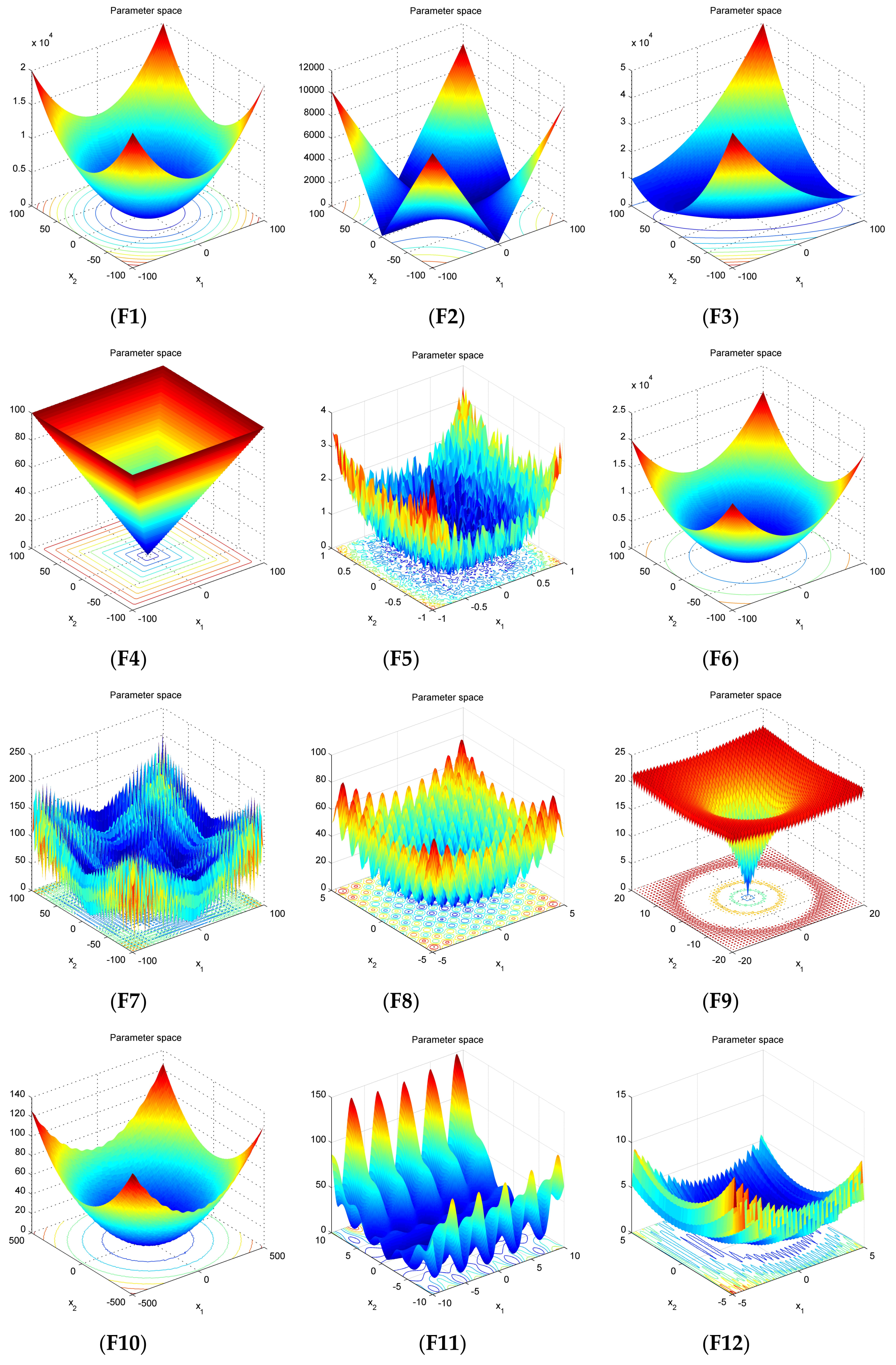
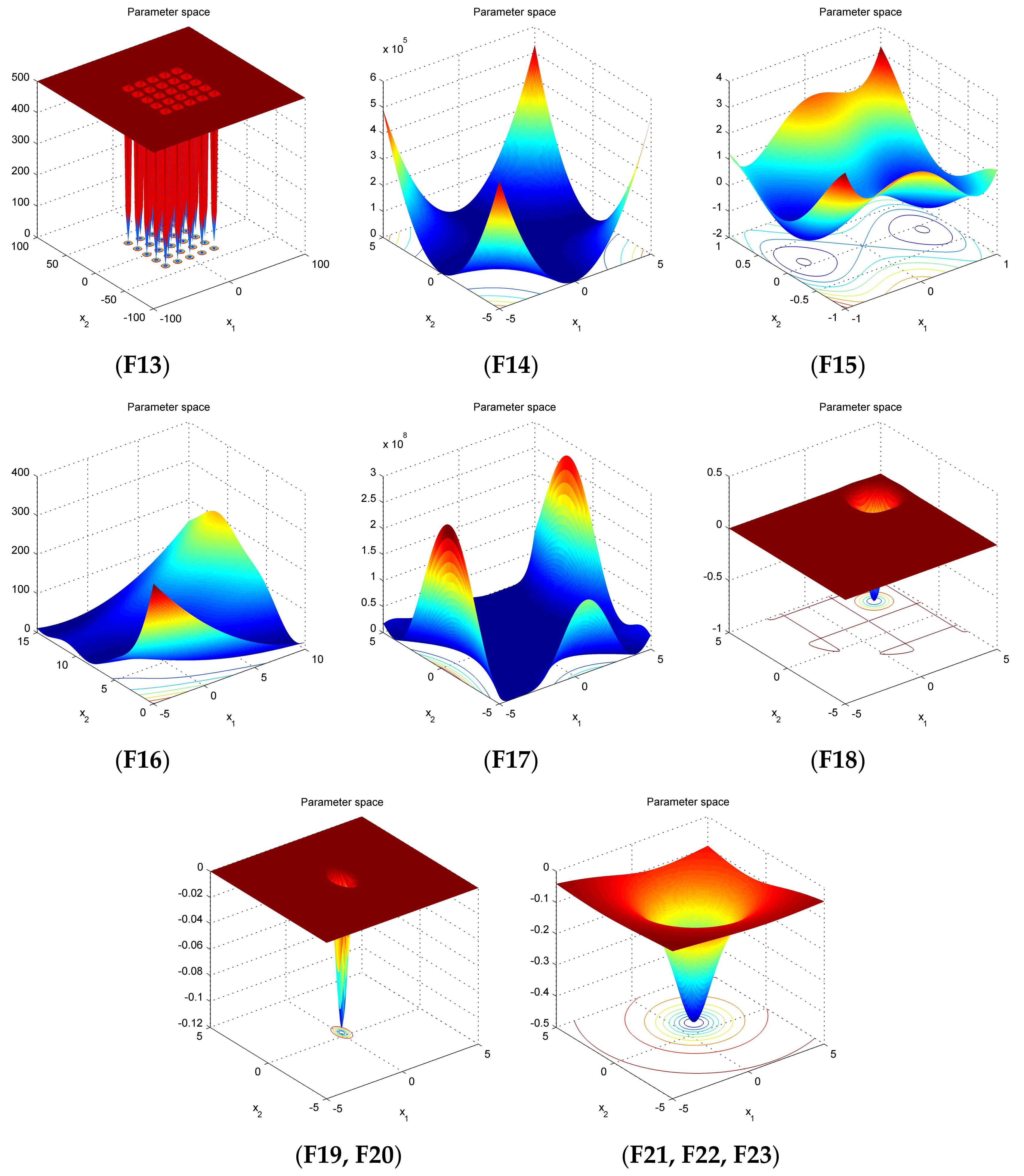
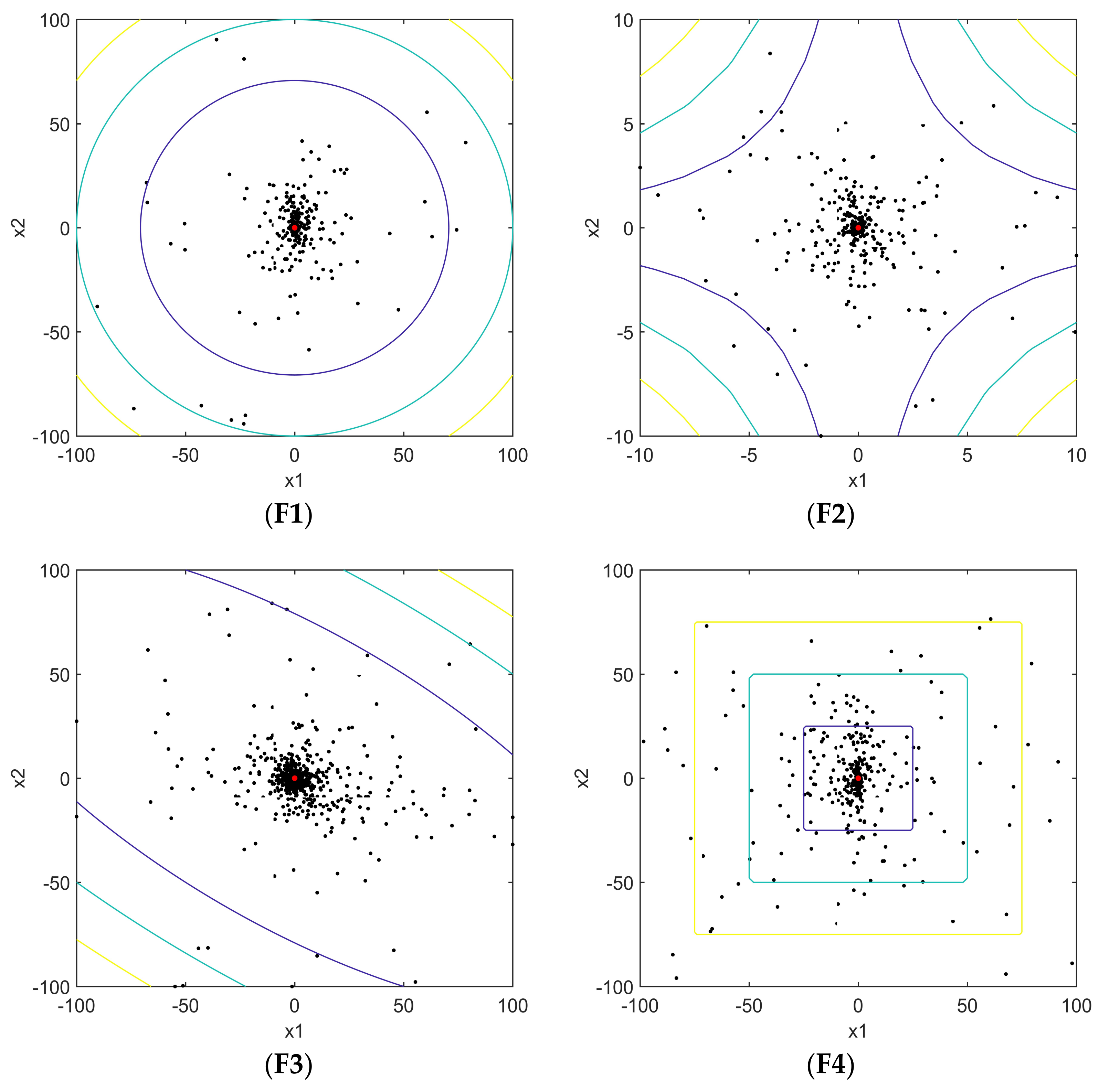
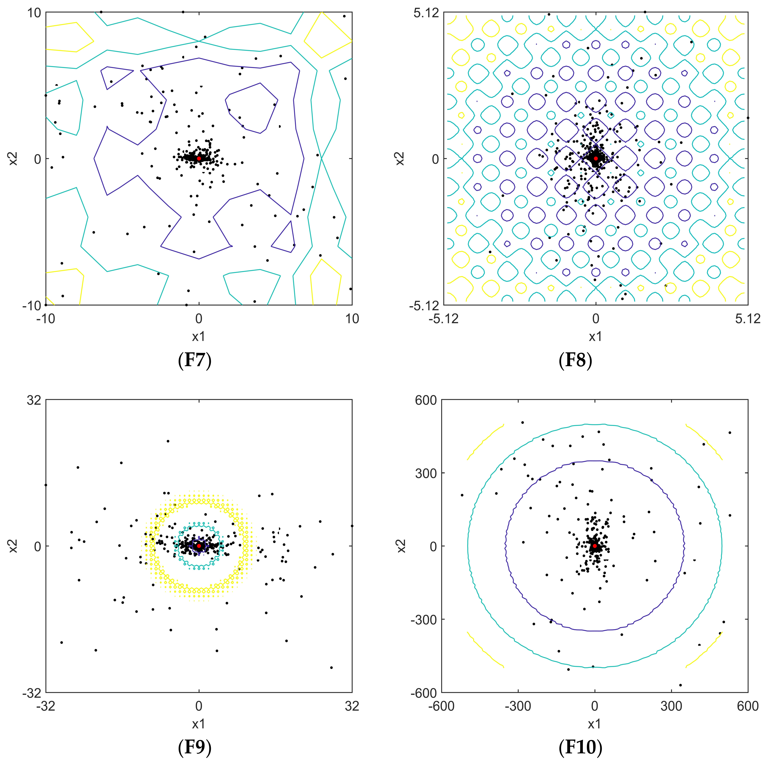
4.1. Benchmark Functions
4.2. Simulation Experiments
4.3. Analysis and Discussion
5. Conclusions and Future Works
Acknowledgments
Author Contributions
Conflicts of Interest
References
- Blum, C.; Aguilera, M.J.B.; Roli, A.; Sampels, M. Hybrid Metaheuristics, an Emerging Approach to Optimization; Springer: Berlin, Germany, 2008. [Google Scholar]
- Raidl, G.R.; Puchinger, J. Combining (Integer) Linear Programming Techniques and Metaheuristics for Combinatorial Optimization; Springer: Berlin/Heidelberg, Germany, 2008; pp. 31–62. [Google Scholar]
- Blum, C.; Cotta, C.; Fernández, A.J.; Gallardo, J.E.; Mastrolilli, M. Hybridizations of Metaheuristics with Branch & Bound Derivates; Springer: Berlin/Heidelberg, Germany, 2008; pp. 85–116. [Google Scholar]
- D’Andreagiovanni, F. On Improving the Capacity of Solving Large-scale Wireless Network Design Problems by Genetic Algorithms. In Applications of Evolutionary Computation. EvoApplications. Lecture Notes in Computer Science; Di Chio, C., Ed.; Springer: Berlin/Heidelberg, Germany, 2011; Volume 6625, pp. 11–20. [Google Scholar]
- D’Andreagiovanni, F.; Krolikowski, J.; Pulaj, J. A fast hybrid primal heuristic for multiband robust capacitated network design with multiple time periods. Appl. Soft. Comput. 2015, 26, 497–507. [Google Scholar] [CrossRef]
- Egea, J.A.; Banga, J.R. Extended ant colony optimization for non-convex mixed integer nonlinear programming. Comput. Oper. Res. 2009, 36, 2217–2229. [Google Scholar]
- Bianchi, L.; Dorigo, M.; Gambardella, L.M.; Gutjahr, W.J. A survey on optimization metaheuristics for stochastic combinatorial optimization. Nat. Comput. 2009, 8, 239–287. [Google Scholar] [CrossRef]
- Cornuéjols, G. Valid inequalities for mixed integer linear programs. Math. Program. 2008, 112, 3–44. [Google Scholar] [CrossRef]
- Murty, K.G. Nonlinear Programming Theory and Algorithms: Nonlinear Programming Theory and Algorithms, 3rd ed.; Wiley: New York, NY, USA, 1979. [Google Scholar]
- Goldberg, D.E. Genetic Algorithms in Search, Optimization and Machine Learning; Addison-Wesley Publishing Company: Boston, MA, USA, 1989; pp. 2104–2116. [Google Scholar]
- Simon, D. Biogeography-Based Optimization. IEEE Trans. Evolut. Comput. 2008, 12, 702–713. [Google Scholar] [CrossRef]
- Storn, R.; Price, K. Differential Evolution—A Simple and Efficient Heuristic for global Optimization over Continuous Spaces. J. Glob. Optim. 1997, 11, 341–359. [Google Scholar] [CrossRef]
- Połap, D.; Woz´niak, M. Polar Bear Optimization Algorithm: Meta-Heuristic with Fast Population Movement and Dynamic Birth and Death Mechanism. Symmetry 2017, 9, 203. [Google Scholar] [CrossRef]
- Bertsimas, D.; Tsitsiklis, J. Simulated Annealing. Stat. Sci. 1993, 8, 10–15. [Google Scholar] [CrossRef]
- Rashedi, E.; Nezamabadi, P.H.; Saryazdi, S. GSA: A Gravitational Search Algorithm. Intell. Inf. Manag. 2012, 4, 390–395. [Google Scholar] [CrossRef]
- Farahmandian, M.; Hatamlou, A. Solving optimization problem using black hole algorithm. J. Comput. Sci. Technol. 2015, 4, 68–74. [Google Scholar] [CrossRef]
- Kaveh, A.; Khayatazad, M. A new meta-heuristic method: Ray Optimization. Comput. Struct. 2012, 112–113, 283–294. [Google Scholar] [CrossRef]
- Kennedy, J.; Eberhart, R. Particle swarm optimization. In Proceedings of the IEEE International Conference on Neural Networks, Perth, Australia, 27 November–1 December 1995; Volume 4, pp. 1942–1948. [Google Scholar]
- Dorigo, M.; Birattari, M.; Stutzle, T. Ant Colony Optimization. IEEE Comput. Intell. Mag. 2007, 1, 28–39. [Google Scholar] [CrossRef]
- Karaboga, D.; Basturk, B. A powerful and efficient algorithm for numerical function optimization: Artificial bee colony (ABC) algorithm. J. Glob. Optim. 2007, 39, 459–471. [Google Scholar] [CrossRef]
- Yang, X.S. Firefly Algorithms for Multimodal Optimization. Mathematics 2010, 5792, 169–178. [Google Scholar]
- Yang, X.S. A New Metaheuristic Bat-Inspired Algorithm. Comput. Knowl. Technol. 2010, 284, 65–74. [Google Scholar]
- Yang, X.S.; Deb, S. Cuckoo Search via Levy Flights. In Proceedings of the World Congress on Nature & Biologically Inspired Computing (NaBIC), Coimbatore, India, 9–11 December 2009; pp. 210–214. [Google Scholar]
- Cuevas, E.; Cienfuegos, M.; Zaldívar, D. A swarm optimization algorithm inspired in the behavior of the social-spider. Expert Syst. Appl. 2014, 40, 6374–6384. [Google Scholar] [CrossRef]
- Mirjalili, S.; Mirjalili, S.M.; Lewis, A. Grey Wolf Optimizer. Adv. Eng. Softw. 2014, 69, 46–61. [Google Scholar] [CrossRef]
- Mirjalili, S. Dragonfly algorithm: A new meta-heuristic optimization technique for solving single-objective, discrete, and multi-objective problems. Neural Comput. Appl. 2016, 27, 1053–1073. [Google Scholar] [CrossRef]
- Mirjalili, S. The Ant Lion Optimizer. Adv. Eng. Softw. 2015, 83, 80–98. [Google Scholar] [CrossRef]
- Mirjalili, S. Moth-flame optimization algorithm: A novel nature-inspired heuristic paradigm. Knowl.-Based Syst. 2015, 89, 228–249. [Google Scholar] [CrossRef]
- Mirjalili, S.; Lewis, A. The Whale Optimization Algorithm. Adv. Eng. Softw. 2016, 95, 51–67. [Google Scholar] [CrossRef]
- Shayeghi, H.; Asefi, S.; Younesi, A. Tuning and comparing different power system stabilizers using different performance indices applying GWO algorithm. In Proceedings of the International Comprehensive Competition Conference on Engineering Sciences, Iran, Anzali, 8 September 2016. [Google Scholar]
- Mohanty, S.; Subudhi, B.; Ray, P.K. A Grey Wolf-Assisted Perturb & Observe MPPT Algorithm for a PV System. IEEE Trans. Energy Conv. 2017, 32, 340–347. [Google Scholar]
- Hameed, I.A.; Bye, R.T.; Osen, O.L. Grey wolf optimizer (GWO) for automated offshore crane design. In Proceedings of the IEEE Symposium Series on Computational Intelligence (SSCI), Athens, Greece, 6–9 December 2017. [Google Scholar]
- Siavash, M.; Pfeifer, C.; Rahiminejad, A. Reconfiguration of Smart Distribution Network in the Presence of Renewable DG’s Using GWO Algorithm. IOP Conf. Ser. Earth Environ. Sci. 2017, 83, 012003. [Google Scholar] [CrossRef]
- Emary, E.; Zawbaa, H.M.; Grosan, C. Experienced Grey Wolf Optimizer through Reinforcement Learning and Neural Networks. IEEE Trans. Neural Netw. Learn. 2018, 29, 681–694. [Google Scholar] [CrossRef] [PubMed]
- Zawbaa, H.M.; Emary, E.; Grosan, C.; Snasel, V. Large-dimensionality small-instance set feature selection: A hybrid bioinspired heuristic approach. Swarm. Evol. Comput. 2018. [Google Scholar] [CrossRef]
- Faris, H.; Aljarah, I.; Al-Betar, M.A. Grey wolf optimizer: A review of recent variants and applications. Neural Comput. Appl. 2017, 22, 1–23. [Google Scholar] [CrossRef]
- Rodríguez, L.; Castillo, O.; Soria, J. A Fuzzy Hierarchical Operator in the Grey Wolf Optimizer Algorithm. Appl. Soft Comput. 2017, 57, 315–328. [Google Scholar] [CrossRef]
- Emary, E.; Zawbaa, H.M.; Hassanien, A.E. Binary Grey Wolf Optimization Approaches for Feature Selection. Neurocomputing 2016, 172, 371–381. [Google Scholar] [CrossRef]
- Emary, E.; Zawbaa, H.M. Impact of chaos functions on modern swarm optimizers. PLoS ONE 2016, 11, e0158738. [Google Scholar] [CrossRef] [PubMed]
- Kohli, M.; Arora, S. Chaotic grey wolf optimization algorithm for constrained optimization problems. J. Comput. Des. Eng. 2017, 1–15. [Google Scholar] [CrossRef]
- Malik, M.R.S.; Mohideen, E.R.; Ali, L. Weighted distance Grey wolf optimizer for global optimization problems. In Proceedings of the 18th IEEE/ACIS International Conference on Software Engineering, Artificial Intelligence, Networking and Parallel/Distributed Computing (SNPD), Kanazawa, Japan, 26–28 June 2017; pp. 1–6. [Google Scholar]
- Heidari, A.A.; Pahlavani, P. An efficient modified grey wolf optimizer with Lévy flight for optimization tasks. Appl. Soft Comput. 2017, 60, 115–134. [Google Scholar] [CrossRef]
- Mittal, N.; Sohi, B.S.; Sohi, B.S. Modified Grey Wolf Optimizer for Global Engineering Optimization. Appl. Comput. Intell. Soft Comput. 2016, 4598, 1–16. [Google Scholar] [CrossRef]
- Muro, C.; Escobedo, R.; Spector, L. Wolf-pack (Canis lupus) hunting strategies emerge from simple rules in computational simulations. Behav. Process. 2011, 88, 192–197. [Google Scholar] [CrossRef] [PubMed]
- Tizhoosh, H.R. Opposition-based learning: A new scheme for machine intelligence. In Proceedings of the International Conference on Computation Intelligence on Modeling Control Automation and International Conference on Intelligent Agents, Web Technologies Internet Commerce, Vienna, Austria, 28–30 November 2005; pp. 695–701. [Google Scholar]
- Rahnamayan, S.; Tizhoosh, H.R.; Salama, M.M.A. Opposition-based differential evolution algorithms. In Proceedings of the IEEE Congress on Evolutionary Computation, Vancouver, BC, Canada, 16–21 July 2006; pp. 2010–2017. [Google Scholar]
- Rahnamayan, S.; Tizhoosh, H.R.; Salama, M.M.A. Opposition-based differential evolution for optimization of noisy problems. In Proceedings of the IEEE Congress on Evolutionary Computation, Vancouver, BC, Canada, 16–21 July 2006; pp. 1865–1872. [Google Scholar]
- Wang, H.; Li, H.; Liu, Y.; Li, C.; Zeng, S. Opposition based particle swarm algorithm with Cauchy mutation. In Proceedings of the IEEE Congress on Evolutionary Computation, Singapore, 25–28 September 2007; pp. 4750–4756. [Google Scholar]
- Rahnamayan, S.; Tizhoosh, H.R.; Salama, M.M.A. Opposition-based differential evolution. IEEE Trans. Evol. Comput. 2008, 2, 64–79. [Google Scholar] [CrossRef]
- Haiping, M.; Xieyong, R.; Baogen, J. Oppositional ant colony optimization algorithm and its application to fault monitoring. In Proceedings of the 29th Chinese Control Conference (CCC), Beijing, China, 29–31 July 2010; pp. 3895–3903. [Google Scholar]
- Lin, Z.Y.; Wang, L.L. A new opposition-based compact genetic algorithm with fluctuation. J. Comput. Inf. Syst. 2010, 6, 897–904. [Google Scholar]
- Shaw, B.; Mukherjee, V.; Ghoshal, S.P. A novel opposition-based gravitational search algorithm for combined economic and emission dispatch problems of power systems. Int. J. Electr. Power Energy Syst. 2012, 35, 21–33. [Google Scholar] [CrossRef]
- Wang, S.W.; Ding, L.X.; Xie, C.W.; Guo, Z.L.; Hu, Y.R. A hybrid differential evolution with elite opposition-based learning. J. Wuhan Univ. (Nat. Sci. Ed.) 2013, 59, 111–116. [Google Scholar]
- Zhao, R.X.; Luo, Q.F.; Zhou, Y.Q. Elite opposition-based social spider optimization algorithm for global function optimization. Algorithms 2017, 10, 9. [Google Scholar] [CrossRef]
- Wang, H.; Wu, Z.; Liu, Y. Space transformation search: A new evolutionary technique. In Proceedings of the First ACM/SIGEVO Summit on Genetic and Evolutionary Computation Conference, Shanghai, China, 12–14 June 2009; pp. 537–544. [Google Scholar]
- Wang, H.; Wu, Z.; Rahnamayan, S. Enhancing particle swarm optimization using generalized opposition-based learning. Inf. Sci. 2011, 181, 4699–4714. [Google Scholar] [CrossRef]
- Wang, H.; Rahnamay, S.; Wu, Z. Parallel differential evolution with self-adapting control parameters and generalized opposition-based learning for solving high-dimensional optimization problems. J. Parallel Distrib. Comput. 2013, 73, 62–73. [Google Scholar] [CrossRef]


| Function | Dim 1 | Range 2 | fmin 3 |
|---|---|---|---|
| F1(x) = | 30 | [−100, 100] | 0 |
| F2(x) = | 30 | [−10, 10] | 0 |
| F3(x) = | 30 | [−100, 100] | 0 |
| F4(x) =ma | 30 | [−100, 100] | 0 |
| F5(x) = | 30 | [−1.28, 1.28] | 0 |
| F6(x) = | 30 | [−100, 100] | 0 |
| F7(x) = | 30 | [−30, 30] | 0 |
| F8(x) = | 30 | [−5.12, 5.12] | 0 |
| F9(x) = | 30 | [−32, 32] | 0 |
| F10(x) = | 30 | [−600, 600] | 0 |
| F11(x) = | 30 | [−50, 50] | 0 |
| F12(x) = | 30 | [−50, 50] | 0 |
| F13(x) = | 2 | [−65, 65] | 1 |
| F14(x) = | 4 | [−5, 5] | 0.00030 |
| F15(x) = 4 | 2 | [−5, 5] | −1.0316 |
| F16(x) = | 2 | [−5, 5] | 0.398 |
| 2 | [−2, 2] | 3 | |
| F18(x) = | 2 | [−100, 100] | −1 |
| F19(x) = | 3 | [1, 3] | −3.86 |
| F20(x) = | 6 | [0, 1] | −3.32 |
| F21(x) = | 4 | [0, 10] | −10.1532 |
| F22(x) = | 4 | [0, 10] | −10.4028 |
| F23(x) = | 4 | [0, 10] | −10.5363 |
| Algorithm | Parameter Values |
|---|---|
| BA | A = 0.25, r = 0.5, f ∈ [0, 2], the population size N = 50 |
| ABC | Limit = 50, the population size N = 50 |
| PSO | Vmax = 6, ωmax = 0.9, ωmin = 0.2, c1 = c2 = 2, the population size N = 50 |
| MFO | a ∈ [−2, −1], the population size N = 50 |
| ALO | w∈ [2, 6] ,the population size N = 50 |
| GWO | a ∈ [0, 2], r1, r2 ∈ rand(), the population size N = 50 |
| DOGWO | a ∈ [0, 2], r1, r2 ∈ rand(), R ∈ rand(), the population size N = 50 |
| Function | Algorithm | Best | Worst | Mean | Std. |
|---|---|---|---|---|---|
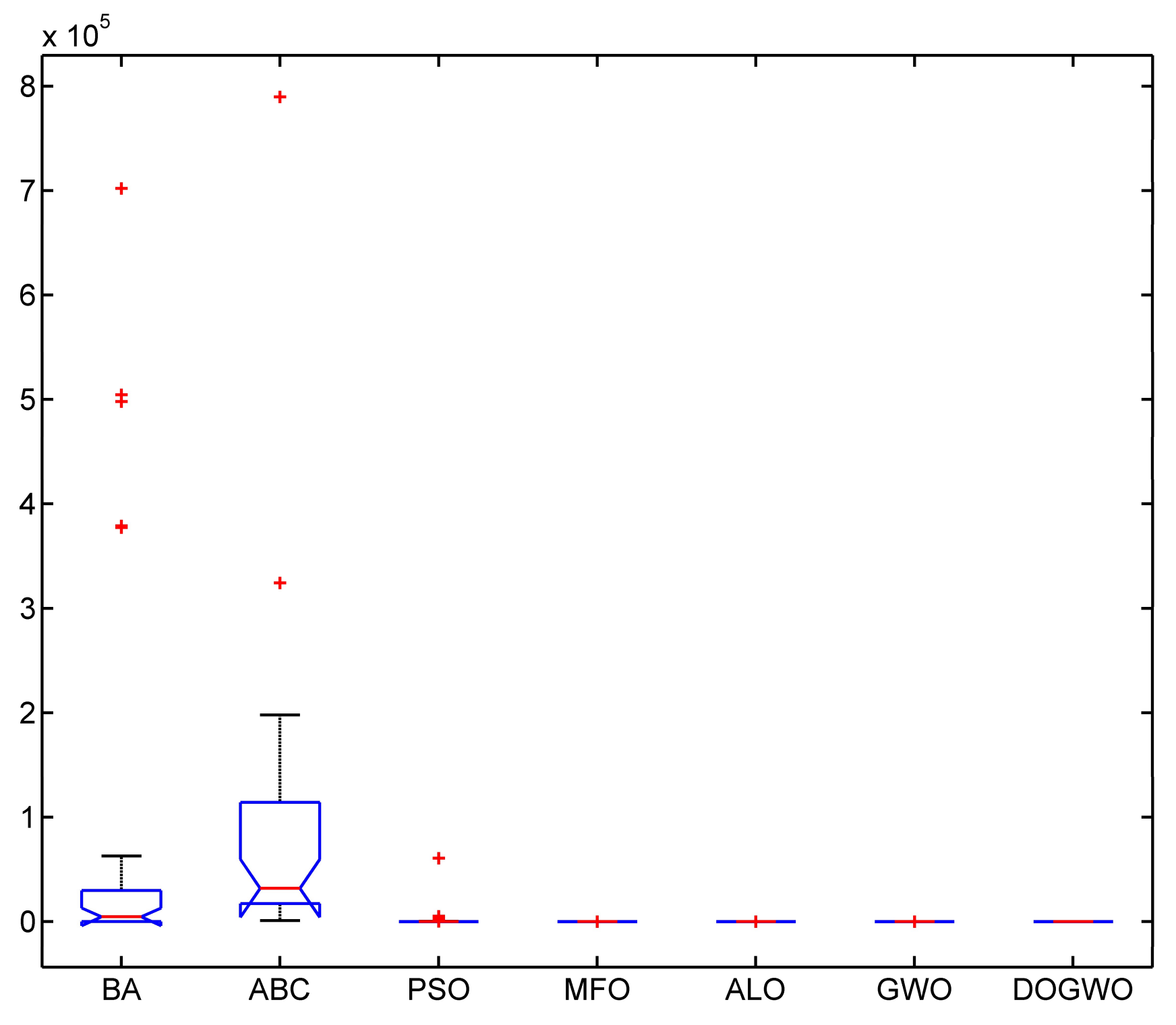
| F1 | BA | 3.27 × | 1.59 × | 7.78 × | 2.97 × |
| ABC | 0.01 | 0.17 | 0.04 | 0.03 | |
| PSO | 0.15 | 5.22 | 1.97 | 1.45 | |
| MFO | 2.72 × | 2.00 × | 3.00 × | 5.35 × | |
| ALO | 1.27 × | 3.94 × | 8.42 × | 9.79 × | |
| GWO | 7.65 × | 1.49 × | 2.24 × | 3.80 × | |
| DOGWO | 0 | 0 | 0 | 0 | |
| F2 | BA | 2.92 | 1.61 × | 9.54 × | 3.33 × |
| ABC | 0.01 | 74.34 | 7.86 | 19.78 | |
| PSO | 0.34 | 2.76 | 1.20 | 0.56 | |
| MFO | 1.12 × | 60.00 | 32.33 | 16.33 | |
| ALO | 0.18 | 124.28 | 31.01 | ||
| GWO | 5.76 × | 5.76 × | 6.09 × | 6.41 × | |
| DOGWO | 0 | 0 | 0 | 0 | |
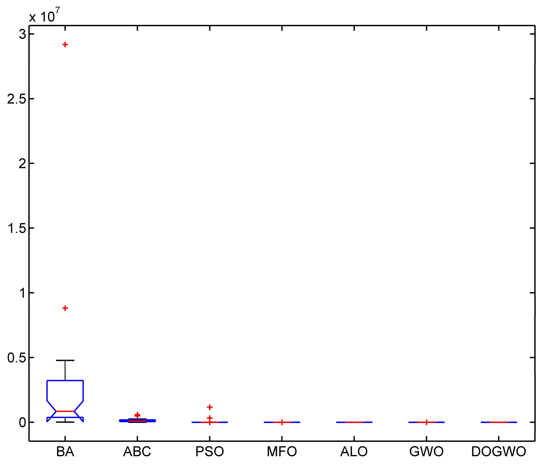
| F3 | BA | 4.86 × | 6.43 × | 2.88 × | 1.56 × |
| ABC | 3.09 × | 7.98 × | 5.86 × | 1.21 × | |
| PSO | 2.33 × | 1.59 × | 7.57 × | 2.74 × | |
| MFO | 2.91 × | 3.84 × | 1.61 × | 1.12 × | |
| ALO | 75.88 | 6.38 × | 2.87 × | 1.47 × | |
| GWO | 5.45 × | 4.12 × | 4.04 × | 9.69 × | |
| DOGWO | 0 | 0 | 0 | 0 | |
| F4 | BA | 26.23 | 56.24 | 37.58 | 7.30 |
| ABC | 47.97 | 61.23 | 54.43 | 3.28 | |
| PSO | 7.59 | 31.43 | 20.47 | 5.08 | |
| MFO | 29.50 | 69.19 | 55.17 | 9.80 | |
| ALO | 3.25 | 15.54 | 8.28 | 2.46 | |
| GWO | 1.26 × | 6.60 × | 1.19 × | 1.14 × | |
| DOGWO | 0 | 0 | 0 | 0 | |
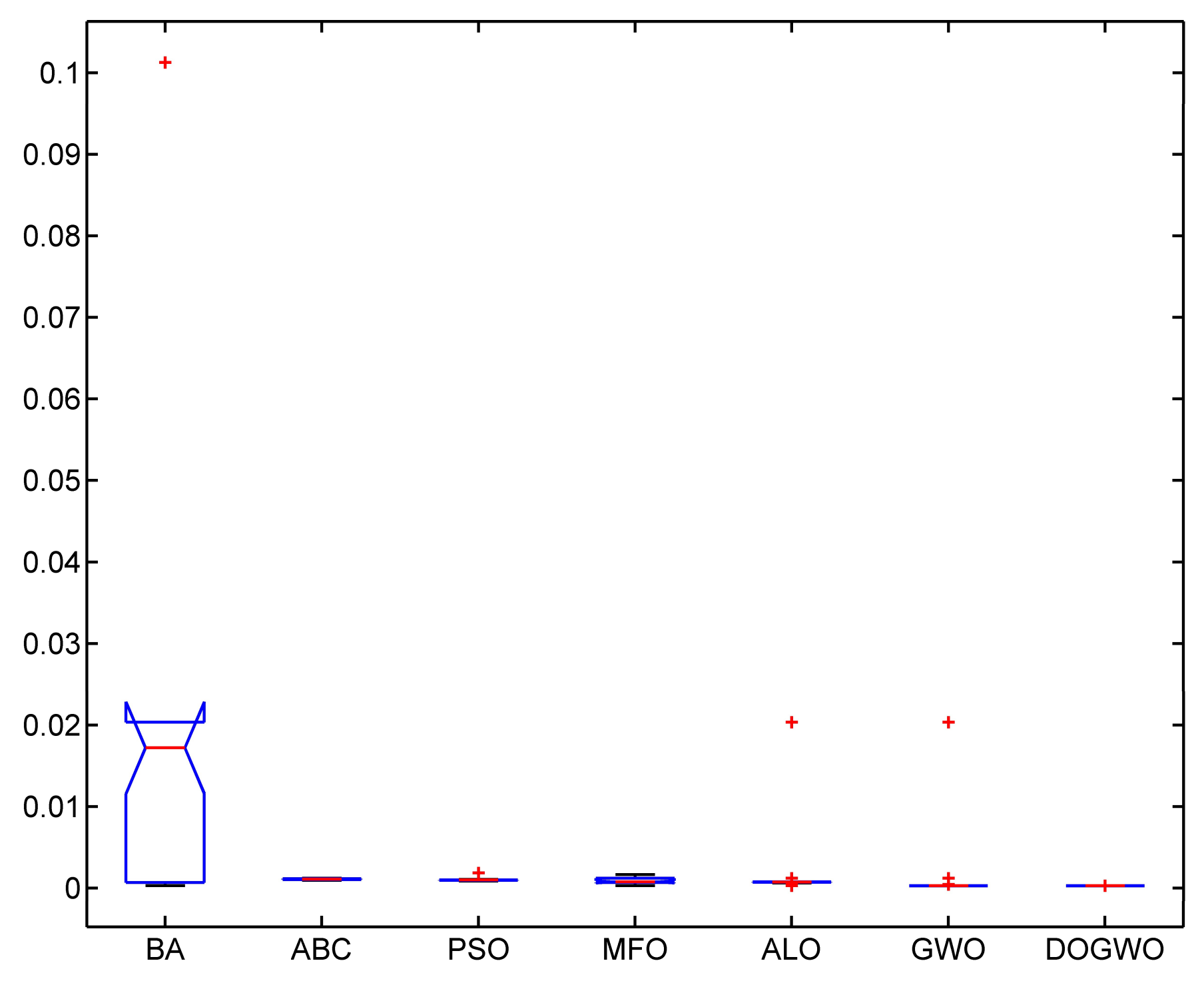
| F5 | BA | 0.53 | 2.84 | 1.54 | 0.57 |
| ABC | 0.09 | 0.25 | 0.17 | 0.05 | |
| PSO | 7.87 | 1.38 × | 73.13 | 42.16 | |
| MFO | 0.02 | 18.86 | 2.12 | 4.09 | |
| ALO | 0.02 | 0.10 | 0.06 | 0.02 | |
| GWO | 1.46 × | 1.09 × | 4.58 × | 2.45 × | |
| DOGWO | 2.07 × | 5.73 × | 2.15 × | 1.67 × | |
| F6 | BA | 4.22 × | 1.29 × | 7.84 × | 2.59 × |
| ABC | 0.01 | 0.11 | 0.04 | 0.02 | |
| PSO | 4.64 | 21.05 | 8.18 | 3.17 | |
| MFO | 5.67 × | 1.01 × | 9.97 × | 3.04 × | |
| ALO | 1.12 × | 1.93 × | 5.60 × | 5.30 × | |
| GWO | 7.48 × | 0.99 | 0.38 | 0.27 | |
| DOGWO | 3.92 × | 0.50 | 0.27 | 0.18 | |
| F7 | BA | 1.12 | 14.02 | 6.44 | 3.12 |
| ABC | 16.59 | 30.05 | 24.25 | 2.68 | |
| PSO | 10.45 | 45.83 | 29.46 | 9.08 | |
| MFO | 7.01 × | 15.32 | 4.39 | 5.56 | |
| ALO | 0.93 | 13.53 | 4.68 | 3.06 | |
| GWO | 4.65 × | 4.87 × | 4.01 × | 1.21 × | |
| DOGWO | 0 | 0 | 0 | 0 | |
| F8 | BA | 1.32 × | 4.97 | 2.08 | 1.51 |
| ABC | 2.05 × | 1.99 × | 5.86 × | 6.26 × | |
| PSO | 0 | 0 | 0 | 0 | |
| MFO | 0 | 0.99 | 0.07 | 0.25 | |
| ALO | 1.07 × | 0.99 | 0.03 | 0.18 | |
| GWO | 0 | 0 | 0 | 0 | |
| DOGWO | 0 | 0 | 0 | 0 | |
| F9 | BA | 11.61 | 16.68 | 14.48 | 1.35 |
| ABC | 0.47 | 2.60 | 1.51 | 0.49 | |
| PSO | 0.44 | 3.23 | 1.27 | 0.71 | |
| MFO | 8.69 × | 19.96 | 14.82 | 8.42 | |
| ALO | 2.22 × | 3.09 | 1.94 | 0.73 | |
| GWO | 7.99 × | 1.51 × | 1.37 × | 2.21 × | |
| DOGWO | 8.88 × | 8.88 × | 8.88 × | 0 | |
| F10 | BA | 62.78 | 1.50× | 1.03× | 21.85 |
| ABC | 0.13 | 0.76 | 0.41 | 0.16 | |
| PSO | 0.31 | 1.01 | 0.67 | 0.19 | |
| MFO | 2.92 × | 90.51 | 6.05 | 22.96 | |
| ALO | 3.95 × | 0.08 | 0.01 | 0.02 | |
| GWO | 0 | 1.62 × | 1.01 × | 4.01 × | |
| DOGWO | 0 | 0 | 0 | 0 | |
| F11 | BA | 10.35 | 7.02 × | 9.05 × | 1.89 × |
| ABC | 9.61 × | 7.89 × | 9.62 × | 1.52 × | |
| PSO | 0.69 | 6.05 × | 2.39 × | 1.10 × | |
| MFO | 2.66 × | 2.48 | 0.28 | 0.52 | |
| ALO | 4.35 | 15.35 | 8.08 | 2.76 | |
| GWO | 6.21 × | 6.01 × | 3.13 × | 1.12 × | |
| DOGWO | 2.54 × | 5.91 × | 2.10 × | 1.01 × | |
| F12 | BA | 4.93 × | 2.92 × | 2.59 × | 1.30 × |
| ABC | 2.05 × | 5.84 × | 1.29 × | 5.39 × | |
| PSO | 0.26 | 1.16 × | 4.97 × | 2.18 × | |
| MFO | 2.65 × | 3.61 | 0.36 | 0.97 | |
| ALO | 2.36 × | 9.82 × | 1.87 × | 0.19 | |
| GWO | 9.86 × | 0.85 | 0.34 | 0.18 | |
| DOGWO | 1.35 × | 0.50 | 0.23 | 0.12 | |
| F13 | BA | 1.992 | 22.90 | 11.13 | 6.28 |
| ABC | 0.998 | 0.998 | 0.998 | 5.14 × | |
| PSO | 0.998 | 3.968 | 1.92 | 1.10 | |
| MFO | 0.998 | 5.93 | 1.59 | 1.18 | |
| ALO | 0.998 | 1.99 | 1.16 | 0.38 | |
| GWO | 0.998 | 12.67 | 3.73 | 4.33 | |
| DOGWO | 0.998 | 2.98 | 1.19 | 0.60 | |
| F14 | BA | 3.07 × | 0.10 | 1.37 × | 1.91 × |
| ABC | 9.39 × | 1.20 × | 1.10 × | 6.98 × | |
| PSO | 8.69 × | 1.90 × | 1.00× | 1.70 × | |
| MFO | 3.09 × | 1.66 × | 9.66 × | 4.04 × | |
| ALO | 3.08 × | 2.04 × | 3.33 × | 6.78 × | |
| GWO | 3.07 × | 2.04 × | 2.30 × | 6.10 × | |
| DOGWO | 3.07 × | 3.07 × | 3.07 × | 7.54 × | |
| F15 | BA | −1.0316 | −1.0316 | −1.0316 | 1.44 × |
| ABC | −1.0316 | −1.0316 | −1.0316 | 1.25 × | |
| PSO | −1.0316 | −1.0315 | −1.0316 | 3.37 × | |
| MFO | −1.0316 | −1.0316 | −1.0316 | 6.78 × | |
| ALO | −1.0316 | −1.0316 | −1.0316 | 5.19 × | |
| GWO | −1.0316 | −1.0316 | −1.0316 | 7.42 × | |
| DOGWO | −1.0316 | −1.0316 | −1.0316 | 3.34 × | |
| F16 | BA | 0.3979 | 0.3979 | 0.3979 | 3.64 × |
| ABC | 0.3979 | 0.3979 | 0.3979 | 8.37 × | |
| PSO | 0.3979 | 0.4136 | 0.3996 | 2.90 × | |
| MFO | 0.3979 | 0.3979 | 0.3979 | 0 | |
| ALO | 0.3979 | 0.3979 | 0.3979 | 3.05 × | |
| GWO | 0.3979 | 0.3979 | 0.3979 | 3.65 × | |
| DOGWO | 0.3979 | 0.3979 | 0.3979 | 4.36 × | |
| F17 | BA | 3 | 3 | 3 | 1.18 × |
| ABC | 3 | 3 | 3 | 8.24 × | |
| PSO | 3 | 3.0003 | 3 | 7.22 × | |
| MFO | 3 | 3 | 3 | 2.68 × | |
| ALO | 3 | 3 | 3 | 1.41 × | |
| GWO | 3 | 3 | 3 | 3.61 × | |
| DOGWO | 3 | 3 | 3 | 1.41 × | |
| F18 | BA | −1 | 0 | −0.2333 | 0.4302 |
| ABC | −1 | −1 | −1 | 1.21 × | |
| PSO | −1 | −0.9982 | −0.9995 | 4.71 × | |
| MFO | −1 | −1 | −1 | 0 | |
| ALO | −1 | −1 | −1 | 7.11 × | |
| GWO | −1 | −1 | −1 | 1.23 × | |
| DOGWO | −1 | −1 | −1 | 1.49 × | |
| F19 | BA | −3.86 | −3.86 | −3.86 | 1.65 × |
| ABC | −3.86 | −3.86 | −3.86 | 1.33 × | |
| PSO | −3.86 | −3.82 | −3.85 | 9.70 × | |
| MFO | −3.86 | −3.86 | −3.86 | 2.71 × | |
| ALO | −3.86 | −3.86 | −3.86 | 1.08 × | |
| GWO | −3.86 | −3.86 | −3.86 | 2.75 × | |
| DOGWO | −3.86 | −3.86 | −3.86 | 2.97 × | |
| F20 | BA | −3.32 | −3.20 | −3.27 | 5.92 × |
| ABC | −3.32 | −3.32 | −3.32 | 8.59 × | |
| PSO | −3.18 | −3.19 | −2.99 | 0.14 | |
| MFO | −3.32 | −3.20 | −3.27 | 5.40 × | |
| ALO | −3.32 | −3.14 | −3.23 | 6.03 × | |
| GWO | −3.32 | −3.09 | −3.24 | 8.09 × | |
| DOGWO | −3.32 | −3.21 | −3.31 | 4.58 × | |
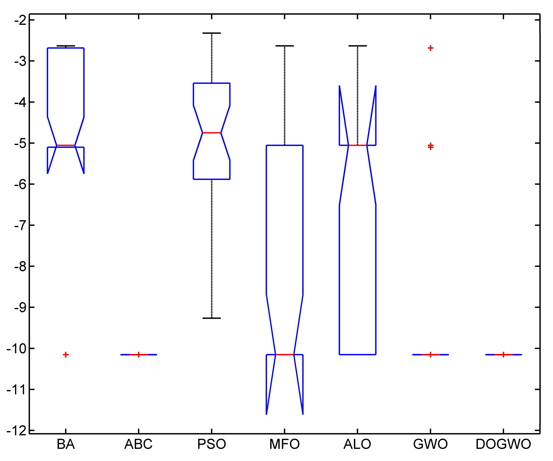
| F21 | BA | −10.1532 | −10.1532 | −10.1532 | 3.006 |
| ABC | −10.1532 | −2.6305 | −5.1363 | 4.52 × | |
| PSO | −10.1532 | −2.3215 | −4.7358 | 1.6195 | |
| MFO | −10.1532 | −2.6305 | −7.9587 | 2.7942 | |
| ALO | −10.1532 | −2.6305 | −6.5294 | 2.9342 | |
| GWO | −10.1531 | −2.6828 | −9.3972 | 1.9975 | |
| DOGWO | −10.1532 | −10.1532 | −10.1532 | 5.81 × | |
| F22 | BA | −10.4029 | −1.8376 | −5.7487 | 3.21 |
| ABC | −10.4029 | −10.4029 | −10.4029 | 6.35 × | |
| PSO | −9.0894 | −2.1988 | −5.0820 | 1.57 | |
| MFO | −10.4029 | −2.7519 | −7.3236 | 3.42 | |
| ALO | −10.4029 | −3.7243 | −8.6734 | 2.71 | |
| GWO | −10.4029 | −5.0877 | −10.0482 | 1.35 | |
| DOGWO | −10.4029 | −10.4029 | −10.4029 | 1.74 × | |
| F23 | BA | −10.5364 | −1.6766 | −5.8869 | 3.66 |
| ABC | −10.5364 | −10.5364 | −10.5364 | 2.41 × | |
| PSO | −9.5666 | −2.3740 | −5.4016 | 1.89 | |
| MFO | −10.5364 | −2.4273 | −9.3062 | 2.81 | |
| ALO | −10.5364 | −2.4273 | −8.2891 | 3.29 | |
| GWO | −10.5364 | −10.5356 | −10.5361 | 1.93 × | |
| DOGWO | −10.5364 | −10.5364 | −10.5364 | 8.12 × |
© 2018 by the authors. Licensee MDPI, Basel, Switzerland. This article is an open access article distributed under the terms and conditions of the Creative Commons Attribution (CC BY) license (http://creativecommons.org/licenses/by/4.0/).
Share and Cite
Xing, Y.; Wang, D.; Wang, L. A Novel Dynamic Generalized Opposition-Based Grey Wolf Optimization Algorithm. Algorithms 2018, 11, 47. https://doi.org/10.3390/a11040047
Xing Y, Wang D, Wang L. A Novel Dynamic Generalized Opposition-Based Grey Wolf Optimization Algorithm. Algorithms. 2018; 11(4):47. https://doi.org/10.3390/a11040047
Chicago/Turabian StyleXing, Yanzhen, Donghui Wang, and Leiou Wang. 2018. "A Novel Dynamic Generalized Opposition-Based Grey Wolf Optimization Algorithm" Algorithms 11, no. 4: 47. https://doi.org/10.3390/a11040047