Evaluating Typical Algorithms of Combinatorial Optimization to Solve Continuous-Time Based Scheduling Problem

Institute of Control Sciences, 65 Profsoyuznaya Street, 117997 Moscow, Russia
*
Authors to whom correspondence should be addressed.
†
These authors contributed equally to this work.
Algorithms 2018, 11(4), 50; https://doi.org/10.3390/a11040050
Submission received: 22 February 2018
/
Revised: 11 April 2018
/
Accepted: 12 April 2018
/
Published: 17 April 2018
(This article belongs to the Special Issue Algorithms for Scheduling Problems)
Abstract
:We consider one approach to formalize the Resource-Constrained Project Scheduling Problem (RCPSP) in terms of combinatorial optimization theory. The transformation of the original problem into combinatorial setting is based on interpreting each operation as an atomic entity that has a defined duration and has to be resided on the continuous time axis meeting additional restrictions. The simplest case of continuous-time scheduling assumes one-to-one correspondence of resources and operations and corresponds to the linear programming problem setting. However, real scheduling problems include many-to-one relations which leads to the additional combinatorial component in the formulation due to operations competition. We research how to apply several typical algorithms to solve the resulted combinatorial optimization problem: enumeration including branch-and-bound method, gradient algorithm, random search technique.
1. Introduction
The Resource-Constrained Project Scheduling Problem (RCPSP) has many practical applications. One of the most obvious and direct applications of RCPSP is planning the fulfilment of planned orders at the manufacturing enterprise [1] that is also sometimes named Job Shop. The Job Shop scheduling process traditionally resides inside the Manufacturing Execution Systems scope [2] and belongs to principle basic management tasks of any industrial enterprise. Historically the Job Shop scheduling problem has two formal mathematical approaches [3]: continuous and discrete time problem settings. In this paper, we research the continuous-time problem setting, analyze its bottlenecks, and evaluate effectiveness of several typical algorithms to find an optimal solution.
The continuous-time Job Shop scheduling approach has been extensively researched and applied in different industrial spheres throughout the past 50 years. One of the most popular classical problem settings was formulated in [4] by Manne as a disjunctive model. This problem setting forms a basic system of restrictions evaluated by different computational algorithms depending on the particular practical features of the model used. A wide overview of different computational approaches to the scheduling problem is conducted in [5,6]. The article [5] considers 69 papers dating back to the XX century, revealing the following main trends in Job Shop scheduling:
- -
- Enumerating techniques
- -
- Different kinds of relaxation
- -
- Artificial intelligence techniques (neural networks, genetic algorithms, agents, etc.)
Artificial intelligence (AI) techniques have become mainstream nowadays. The paper [6] gives a detailed list of AI techniques and methods used for scheduling.
From the conceptual point of view, this paper deals with a mixed integer non-linear (MINLP) scheduling problem [5] that is relaxed to a combinatorial set of linear programming problems due to the linear “makespan” objective function. As a basic approach we take the disjunctive model [4]. A similar approach was demonstrated in [7] where the authors deployed the concept of parallel dedicated machines scheduling subject to precedence constraints and implemented a heuristic algorithm to generate a solution.
2. Materials and Methods
In order to formalize the continuous-time scheduling problem we will need to introduce several basic definitions and variables. After that, we will form a system of constraints that reflect different physical, logical and economic restrictions that are in place for real industrial processes. Finally, introducing the objective function will finish the formulation of RCPSP as an optimization problem suitable for solving.
2.1. Notions and Base Data for Scheduling
Sticking to the industrial scheduling also known as the Job Shop problem, let us define the main notions that we will use in the formulation:
- The enterprise functioning process utilizes resources of different types (for instance machines, personnel, riggings, etc.). The set of the resources is indicated by a variable , .
- The manufacturing procedure of the enterprise is formalized as a set of operations J tied with each other via precedence relations. Precedence relations are brought to a matrix , , . Each element of the matrix iff the operation j follows the operation i and zero otherwise .
- Each operation i is described by duration . Elements , , form a vector of operations’ durations ⟶.
- Each operation i has a list of resources it uses while running. Necessity for resources for each operation is represented by the matrix , , . Each element of the matrix iff the operation i of the manufacturing process allocates the resource r. All other cases bring the element to zero value .
- The input orders of the enterprise are considered as manufacturing tasks for the certain amount of end product and are organized into a set F. Each order is characterized by the end product amount and the deadline , . Elements inside F are sorted in the deadline ascending order.
Using the definitions introduced above, we can now formalize the scheduling process as residing all operations of all orders on the set of resources R. Mathematically this means defining the start time of each operation of each order .
2.2. Continuous-Time Problem Setting
The continuous-time case is formulated around the variables that stand for the start moments of each operation i of each order f: , , [3]. The variables can be combined into vectors . The main constraints of the optimization problem in that case are:
- Precedence graph of the manufacturing procedure:
- Meeting deadlines for all orders
The constraints above do not take into consideration the competition of operations that try to allocate the same resource. We can distinguish two types of competition here: competition of operations within one order and competition of operations of different orders. The competition of operations on parallel branches of one order is considered separately by modelling the scheduling problem for a single order (this is out of the scope of this paper). The main scope of this research is to address the competition of operations from different orders. Assuming we have the rule (constraint) that considers the competition of operations within one and the same order let us formalize the competition between the operations of different orders. Consider we have a resource, which is being allocated by K different operations of different orders.
For each resource let us distinguish only those operations that allocate it during their run. The set of such operations can be found from the corresponding column of the resource allocation matrix , , .
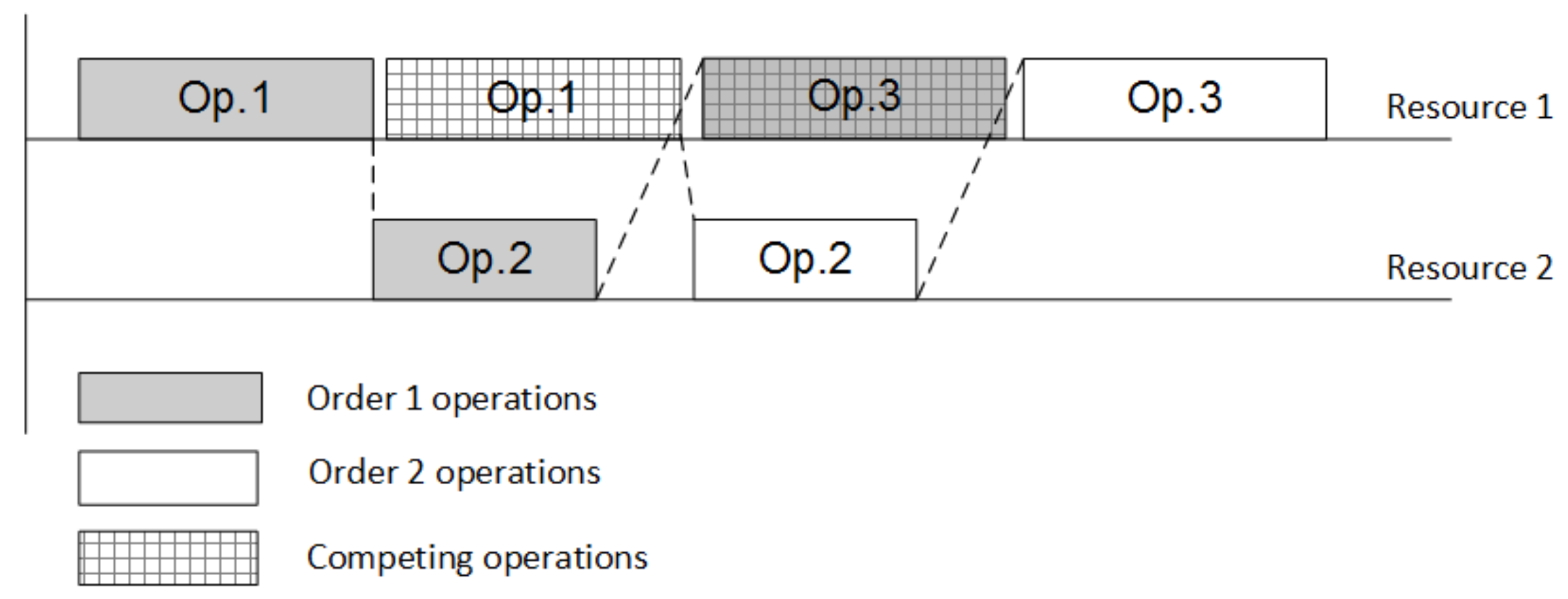
The example for two competing operations of two different orders is shown in Figure 1.
For each resource each competing operation of order will compete with all other competing operations of all other orders, i.e., going back to the example depicted in Figure 1 we will have the following constraint for each pair of operations:
where indexes are as follows ; ; . Implementing an additional Boolean variable will convert each pair of constraints into one single formula:
From the above precedence constraints, we can form the following set of constraints for the optimization problem:
where the variables are continuous and represent the start times of each operation of each order; and variables are Boolean and represent the position of each competing operation among other competitors for each resource.
2.3. Combinatorial Optimization Techniques
From the mathematical point of view, the resulting basic problem setting belongs to linear programming class. The variables , form a combinatorial set of subordinate optimization problems [8]. However, we must suppress that the combinatorial set , , is not full as the sequence of operations within each order is dictated by manufacturing procedure. Consequently, the number of combinations is restricted only to those variants when the operations of different orders trade places without changing their queue within one order. Let us research possible ways to solve the given combinatorial set of problems. In this article, the optimization will be conducted with “makespan” criterion formalized with the formula:
2.3.1. Enumeration and Branch-and-Bound Approach
Enumerating the full set of combinations for all competing operations is an exercise of exponential complexity [9]. However, as we have mentioned above the number of combinations in constraint (3) is restricted due to other constraints (2) and (1). The precedence graph constraint (1) excludes the permutations of competing operations within one order making the linear problem setting non-feasible for corresponding combinations. The way we enumerate the combinations and choose the starting point of enumeration also influences the flow of computations significantly. The common approach to reducing the number of iterations in enumeration is to detect the forbidden areas where the optimal solution problem does not exist (e.g., the constraints form a non-feasible problem or multiple solutions exist). The most widely spread variant of the technique described is branch-and-bound method [10] and its different variations.
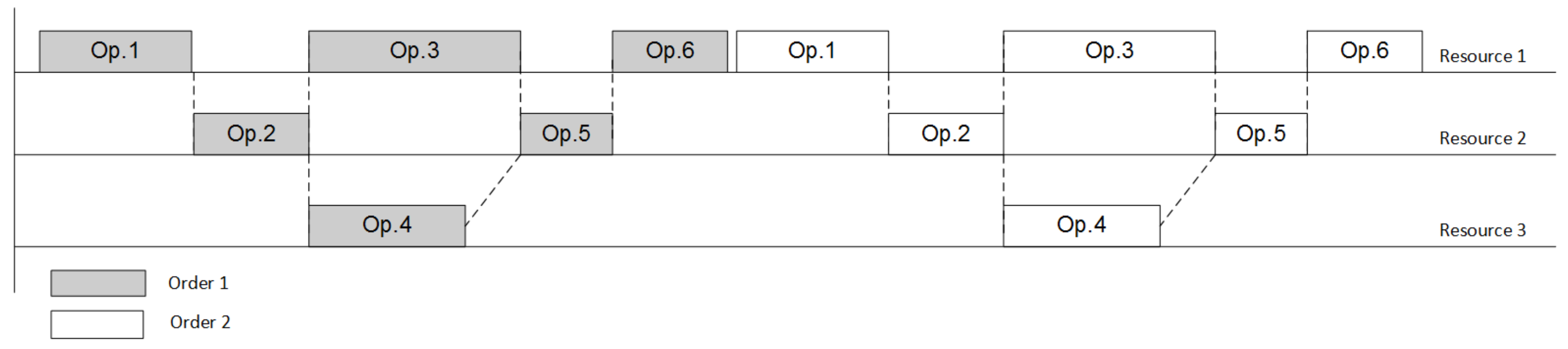
Let us choose the strategy of enumerating permutations of operations in such a way that it explicitly and easily affords to apply branch-and-bound method. The starting point of the enumeration will be the most obvious positioning of orders in a row as shown in Figure 2. We start from the point where the problem is guaranteed to be solvable—when all orders are planned in a row—which means that the first operation of the next order starts only after the last operation of the previous order is finished. If the preceding graph is correct and the resources are enough that means the single order can be placed on the resources that are totally free (the problem is solvable—we do not consider the unpractical case when the graph and/or resources are not enough to fulfill a single order). Infeasibility here can be reached only in the case when we start mixing the orders. This guarantees that the linear programming problem is solvable, however, this combination is far from being optimal/reasonable.
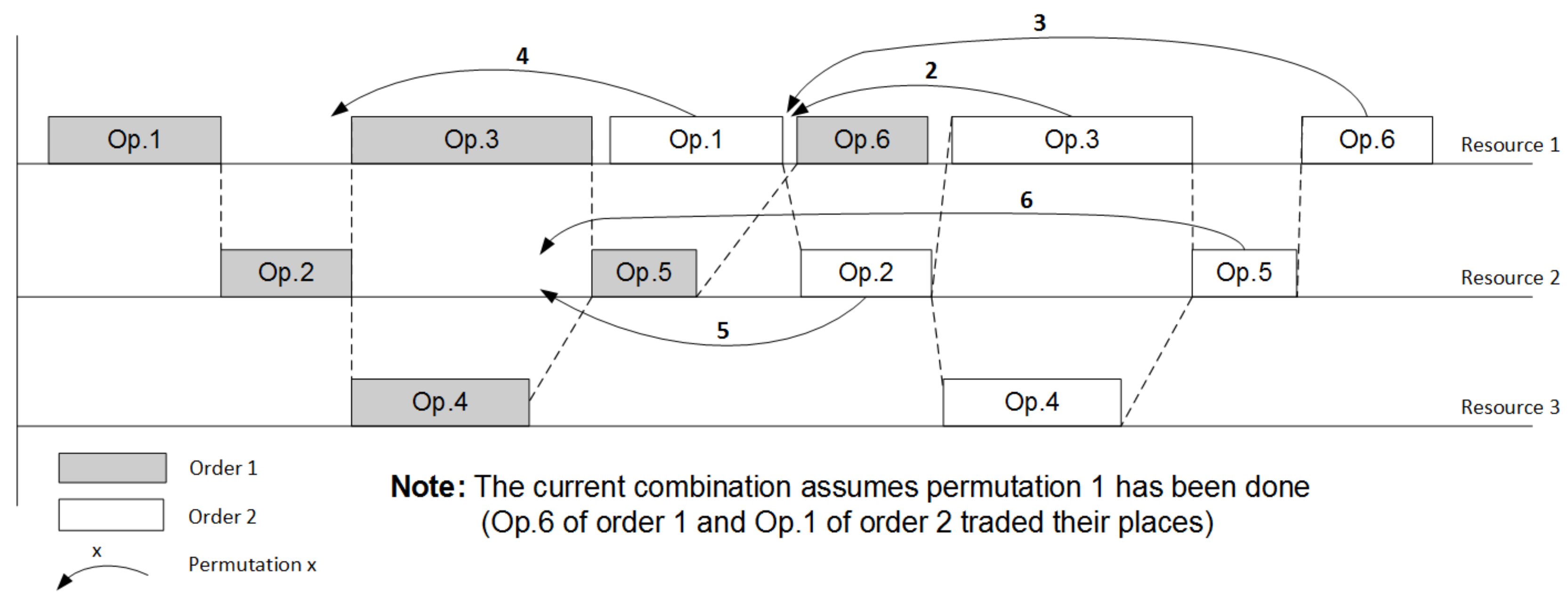
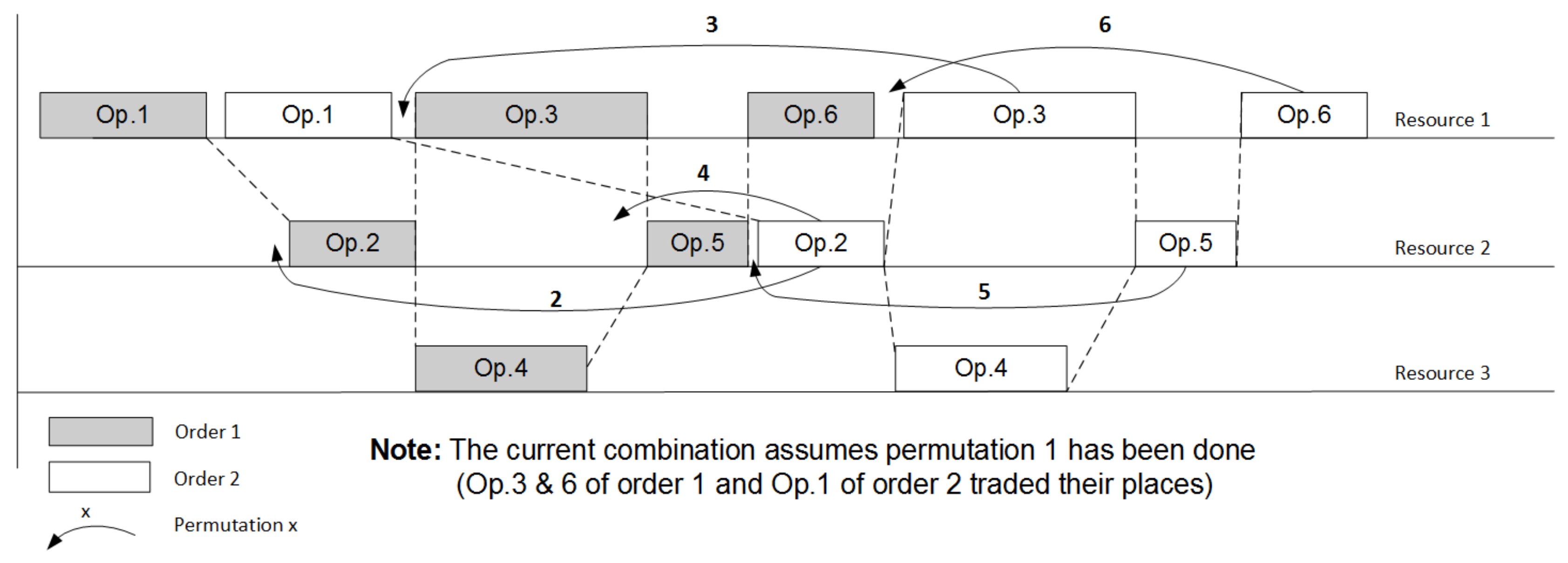
The enumeration is organized by shifting the operations of the last order to the left in such a way that they trade their places with previous competing operations of preceding orders (see Figure 3). As soon as the operation reaches its leftmost feasible position and the current combination corresponds to a linear programming problem with no solution we roll back to the previous combination, stop shifting operations of the last order and switch to the operations of the previous order. After the enumeration for orders on the current resource is over, we proceed the same iterations with the next resource. The formal presentation of the designed branch-and-bound algorithm is described by Procedure 1.
Procedure 1: branch-and-bound 1. Find the initial solution of the LP problem (1)–(3) for the combination , that corresponds to the case when all orders are in a row (first operation of the following order starts only after the last operation of preceding order is completed). 2. Remember the solution and keep the value of objective function as temporarily best result . 3. Select the last order . 4. Select the resource that is used by last operation of the precedence graph G of the manufacturing process. 5. The branch is now formulated. 6. Condition: Does the selected resource r have more than one operation in the manufacturing procedure that allocates it? 6.1. If yes then Begin evaluating branch Shift the operation i one competing position to the left Find the solution of the LP problem (1)–(3) for current combination and calculate the objective function Condition: is the solution feasible? If feasible then Condition: Is the objective function value better than temporarily best result ? If yes then save current solution as the new best result . End of condition Switch to the preceding operation of currently selected order f for the currently selected resource r. Go to the p. 5 and start evaluating the new branch If not feasible then Stop evaluating branch Switch to the preceding resource Go to the p. 5 and start evaluating the new branch End of condition: is the solution feasible? End of condition: p. 6 7. Switch to the preceding order 8. Repeat pp. 4–7 until no more branches are available 9. Repeat pp. 3–8 until no more feasible shifts are possible for all operations in all branches.
Iterating combinations for one order on one resource can be considered as evaluating one branch of the algorithm [10]. Finding the leftmost position for an operation is similar to detecting a bound. Switching between branches and stopping on bounds is formalized with a general branch-and-bound procedure.
2.3.2. Gradient-Alike Algorithm
The opposite of the mentioned above approach would be searching for a local minimum among all combinations with a gradient algorithm [11]. Here, we will compute an analogue of the derivative that is used to define the search direction at each point [12]. ‘Derivative’ for each competing operation is calculated by trying to shift it by one position to the left. In case the objective function reduces (or increases for maximization problems) we shift the operation to the left with the defined step (the step ratio is measured in a number of position operation skips moving to the left). The formal presentation of the designed gradient-alike algorithm is described by Procedure 2.
Procedure 2: gradient algorithm 1. Find the initial solution of the LP problem (1)–(3) for the combination , that corresponds to the case when all orders are in a row (first operation of the following order starts only after the last operation of preceding order is completed). 2. Remember the solution and keep the value of objective function as temporarily best result . 3. Select the last order . 4. Select the resource that is used by first operation of the sequence graph of the manufacturing process. 5. The current optimization variable for gradient optimization is selected—position of operation i of the order f on the resource r. 6. Condition: Does the selected resource r have more than one operation in the manufacturing procedure that allocates it? 6.1. If yes then Begin optimizing position 6.1.1. Set the step of shifting the operation to maximum (shifting to the leftmost position). 6.1.2. Find the ‘derivative’ of shifting the operation i to the left Shift the operation i one position to the left Find the solution of the LP problem (1)–(3) for current combination and calculate the objective function Condition A: is the solution feasible? If feasible then Condition B: Is the objective function value better than temporarily best result ? If yes then We found the optimization direction for position , proceed to p. 6.1.3 If not then No optimization direction for the current position stop optimizing position switch to the next operation go to p 6 and repeat search for position End of condition B If not feasible then No optimization direction for the current position stop optimizing position switch to the next operation go to p 6 and repeat search for position End of condition A 6.1.3. Define the maximum possible optimization step for the current position , initial step value Shift the operation i left using the step . Find the solution of the LP problem (1)–(3) for current combination and calculate the objective function Condition C: Is the solution feasible and objective function value better than temporarily best result ? If yes then save current solution as the new best result stop optimizing position switch to the next operation go to p 6 and repeat search for position If not then reduce the step twice and repeat operations starting from p. 6.1.3 End of condition C Switch to the next operation, go to p. 6 and optimize position 7. Switch to the preceding resource 8. Repeat pp. 5–7 for currently selected resource 9. Switch to the preceding order 10. Repeat pp. 4–9 for currently selected order . 11. Repeat pp. 3–10 until no improvements and/or no more feasible solutions exist.
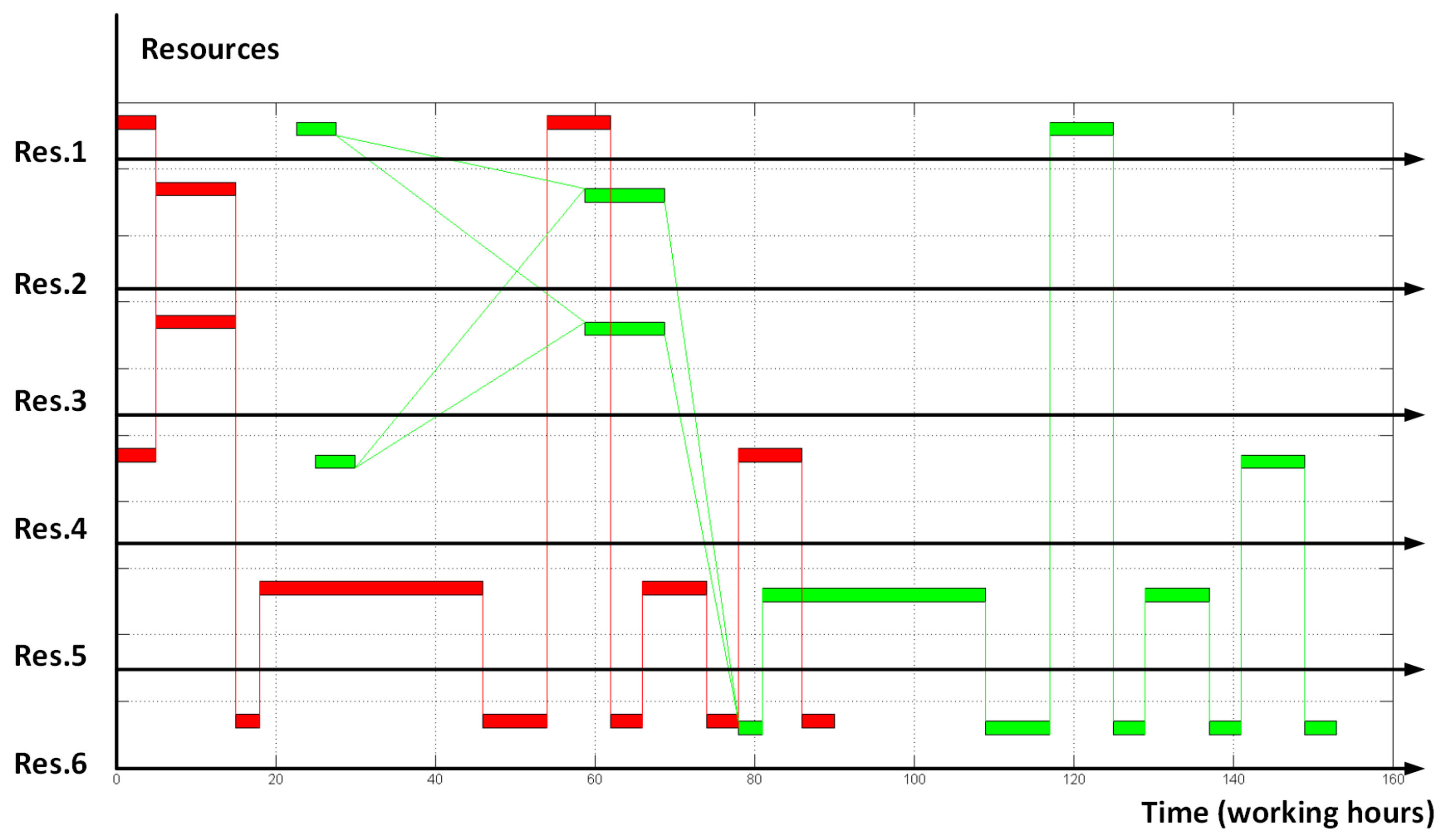
The optimization variables in gradient algorithm represent positions of all competing operations relative to each other. The maximum optimization step for each iteration is detected on-the-fly by trying to shift the current operation to the leftmost position (as it is shown in Figure 4) that shows the LP problem (1)–(3) is solvable and the objective function is improved.
3. Results of the Computational Experiment
As a reference trial example let us take the following scheduling problem. The manufacturing procedure contains 13 operations that require 6 different resources. The schedule of the manufacturing procedure for a single order is shown in Figure 5. In this example, we want to place two orders at the depicted resources and start evaluating from the point ‘all orders in a row’ (see Figure 6).
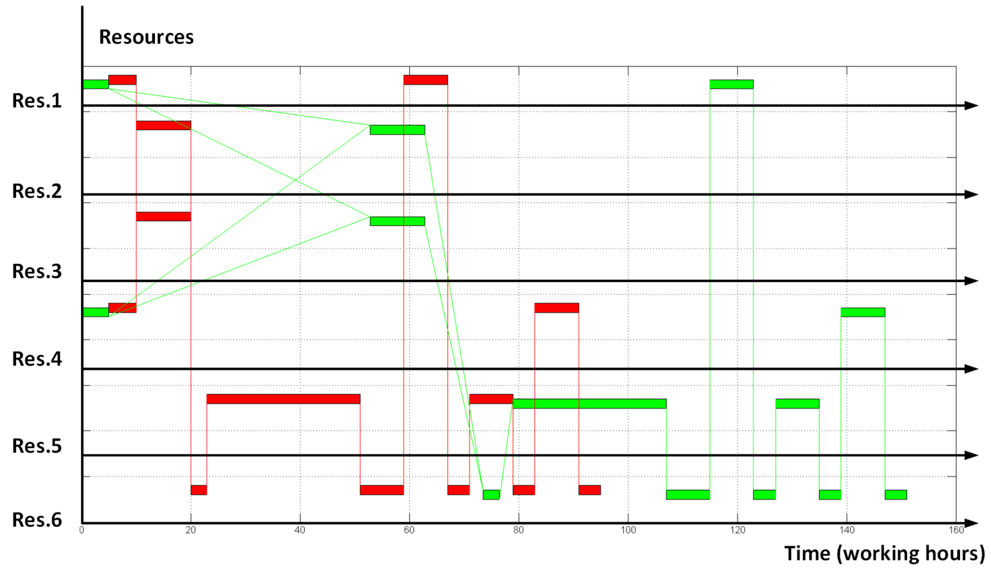
The results of evaluating branch-and-bound and gradient algorithm are placed in the following Table 1. The resulting schedules are depicted in Figure 7 (for branch-and-bound algorithm) and Figure 8 (for gradient algorithm).
Results of analysis gives us understanding that for a modest dimensionality scheduling problem both considered approaches are applicable. However, as the number of operations in manufacturing procedure grows and the number of orders increases, we will experience an enormous growth of algorithm iterations for enumeration (branch-and-bound) technique and the gradient-alike algorithm will obviously detect local optimum as the best achievable solution (which means the optimization results will differ more and more compared to the digits in Table 1). Rising difference between the results is shown in Table 2.
Expanding the previous problem for a procedure of 500 operations in 2 orders we will get the results presented in Table 3.
4. Discussion
Analyzing the computational experiment result, we come to a classical research outcome that to solve the global optimization problem effectively we need to find a more computationally cheap algorithm that gives a solution closer to global optimum. Let us try several standard approaches to improve the solution with non-exponential algorithm extensions.
4.1. Random Search as an Effort to Find Global Optimum
As mentioned above, the gradient algorithm, being more effective from the computational complexity point of view, affords to find only local suboptimal solutions [12]. A typical extension to overcome this restriction would be random search procedure. The main idea of this modification is to iterate gradient search multiple times going out from different starting points [13]. In case the starting points are generated randomly we can assume that the more repeating gradient searches we do the higher the probability of finding a global optimum we achieve. There was some research conducted in this area whose outcome recommends how many starting points to generate in order to cover the problem’s acceptance region with high value of probability [14]. According to [14] the acceptable number of starting points is calculated as
where , and is the dimensionality of optimization problem being solved, i.e., for our case this is the number of all competing operations of all orders on all resources. The result of applying random search approach is represented in Table 2.
The main barrier for implementing the random search procedure for the combinatorial scheduling problem is generating enough feasible optimization starting points. As we can see from the results in Table 2, number of failures to generate feasible starting point is much higher than the quantity of successful trials. Leaning upon the results of enumeration algorithm in Table 1 we can assume that the tolerance regions for optimization problem (1)–(3) are very narrow. Even from the trial example in Table 1 we see that the number of feasible iterations (25) collect less than 10 percent of all possible permutations (318) which leaves us very low probability of getting a feasible initial point for further gradient optimization. Thus, we can make a conclusion that ‘pure’ implementation of random search procedure will not give a huge effect but should be accompanied with some analytic process of choosing feasible initial points of optimization. Such a procedure may be based on non-mathematical knowledge such as industry or management expertise. From our understanding, this question should be investigated separately.
5. Conclusions
Research of a continuous-time scheduling problem is conducted. We formalized the scheduling problem as a combinatorial set [8] of linear programming sub problems and evaluated typical computational procedures with it. In addition to the classical and estimated resulting conflict between the “complexity” and “locality” of optimization algorithms we came to the conclusion that the classical approach of randomization is unhelpful in terms of improving the locally found suboptimal solution. The reason here is that the scheduling problem in setting (1)–(3) has a very narrow feasibility area which makes it difficult to randomly detect a sufficient number of starting points for further local optimization. The efficiency of random search might be increased by introducing a martial rule or procedure of finding typical feasible starting points. The other effective global optimization procedures are mentioned in a very short form and are left for further authors’ research. They are:
- Genetic algorithms. From the first glance evolutionary algorithms [15] should have a good application case for the scheduling problem (1)–(3). The combinatorial vector of permutations , , seems to be naturally and easily represented as a binary crossover [15] while the narrow tolerance region of the optimization problem will contribute to the fast convergence of the breeding procedure. Authors of this paper leave this question for further research and discussion.
- Dynamic programming. A huge implementation area in global optimization (and particularly in RCPSP) is left for dynamic programming algorithms [16]. Having severe limitations in amount and time we do not cover this approach but will come back to it in future papers.
The computation speed of the high dimension problem using an average PC is not satisfactory. This fact forces authors to investigate parallel computing technologies. Future research assumes adoption of created algorithms to a parallel paradigm, for instance, implementing map-reduce technology [17].
Acknowledgments
This work was supported by the Russian Science Foundation (grant 17-19-01665).
Author Contributions
A.A.L. conceived conceptual and scientific problem setting; I.N. adopted the problem setting for manufacturing case and designed the optimization algorithms; N.P. implemented the algorithms, performed the experiments and analyzed the data.
Conflicts of Interest
The authors declare no conflict of interest. The founding sponsors had no role in the design of the study; in the collection, analyses, or interpretation of data; in the writing of the manuscript, and in the decision to publish the results.
References
- Artigues, C.; Demassey, S.; Néron, E.; Sourd, F. Resource-Constrained Project Scheduling Models, Algorithms, Extensions and Applications; Wiley-Interscience: Hoboken, NJ, USA, 2008. [Google Scholar]
- Meyer, H.; Fuchs, F.; Thiel, K. Manufacturing Execution Systems. Optimal Design, Planning, and Deployment; McGraw-Hill: New York, NY, USA, 2009. [Google Scholar]
- Jozefowska, J.; Weglarz, J. Perspectives in Modern Project Scheduling; Springer: New York, NY, USA, 2006. [Google Scholar]
- Manne, A.S. On the Job-Shop Scheduling Problem. Oper. Res. 1960, 8, 219–223. [Google Scholar] [CrossRef]
- Jones, A.; Rabelo, L.C. Survey of Job Shop Scheduling Techniques. In Wiley Encyclopedia of Electrical and Electronics Engineering; National Institute of Standards and Technology: Gaithersburg, ML, USA, 1999. Available online: http://citeseerx.ist.psu.edu/viewdoc/download?doi=10.1.1.37.1262&rep=rep1&type=pdf (accessed on 10 April 2017).
- Taravatsadat, N.; Napsiah, I. Application of Artificial Intelligent in Production Scheduling: A critical evaluation and comparison of key approaches. In Proceedings of the 2011 International Conference on Industrial Engineering and Operations Management, Kuala Lumpur, Malaysia, 22–24 January 2011; pp. 28–33. [Google Scholar]
- Hao, P.C.; Lin, K.T.; Hsieh, T.J.; Hong, H.C.; Lin, B.M.T. Approaches to simplification of job shop models. In Proceedings of the 20th Working Seminar of Production Economics, Innsbruck, Austria, 19–23 February 2018. [Google Scholar]
- Trevisan, L. Combinatorial Optimization: Exact and Approximate Algorithms; Stanford University: Stanford, CA, USA, 2011. [Google Scholar]
- Wilf, H.S. Algorithms and Complexity; University of Pennsylvania: Philadelphia, PA, USA, 1994. [Google Scholar]
- Jacobson, J. Branch and Bound Algorithms—Principles and Examples; University of Copenhagen: Copenhagen, Denmark, 1999. [Google Scholar]
- Erickson, J. Models of Computation; University of Illinois: Champaign, IL, USA, 2014. [Google Scholar]
- Ruder, S. An Overview of Gradient Descent Optimization Algorithms; NUI Galway: Dublin, Ireland, 2016. [Google Scholar]
- Cormen, T.H.; Leiserson, C.E.; Rivest, R.L.; Stein, C. Introduction to Algorithms, 3rd ed.; Massachusetts Institute of Technology: London, UK, 2009. [Google Scholar]
- Kalitkyn, N.N. Numerical Methods; Chislennye Metody; Nauka: Moscow, Russia, 1978. (In Russian) [Google Scholar]
- Haupt, R.L.; Haupt, S.E. Practical Genetic Algorithms, 2nd ed.; Wiley-Interscience: Hoboken, NJ, USA, 2004. [Google Scholar]
- Mitchell, I. Dynamic Programming Algorithms for Planning and Robotics in Continuous Domains and the Hamilton-Jacobi Equation; University of British Columbia: Vancouver, BC, Canada, 2008. [Google Scholar]
- Miner, D.; Shook, A. MapReduce Design Patterns: Building Effective Algorithms and Analytics for Hadoop and Other Systems; O’Reilly Media: Sebastopol, CA, USA, 2013. [Google Scholar]
Figure 1.
Competing operations on one resource.

Figure 2.
Initial state: all orders are placed in a row.

Figure 3.
Permutations of competing operations in branch-and-bound algorithm.

Figure 4.
Permutations of competing operations in gradient algorithm.

Figure 5.
Gannt diagram for single order manufacturing procedure.
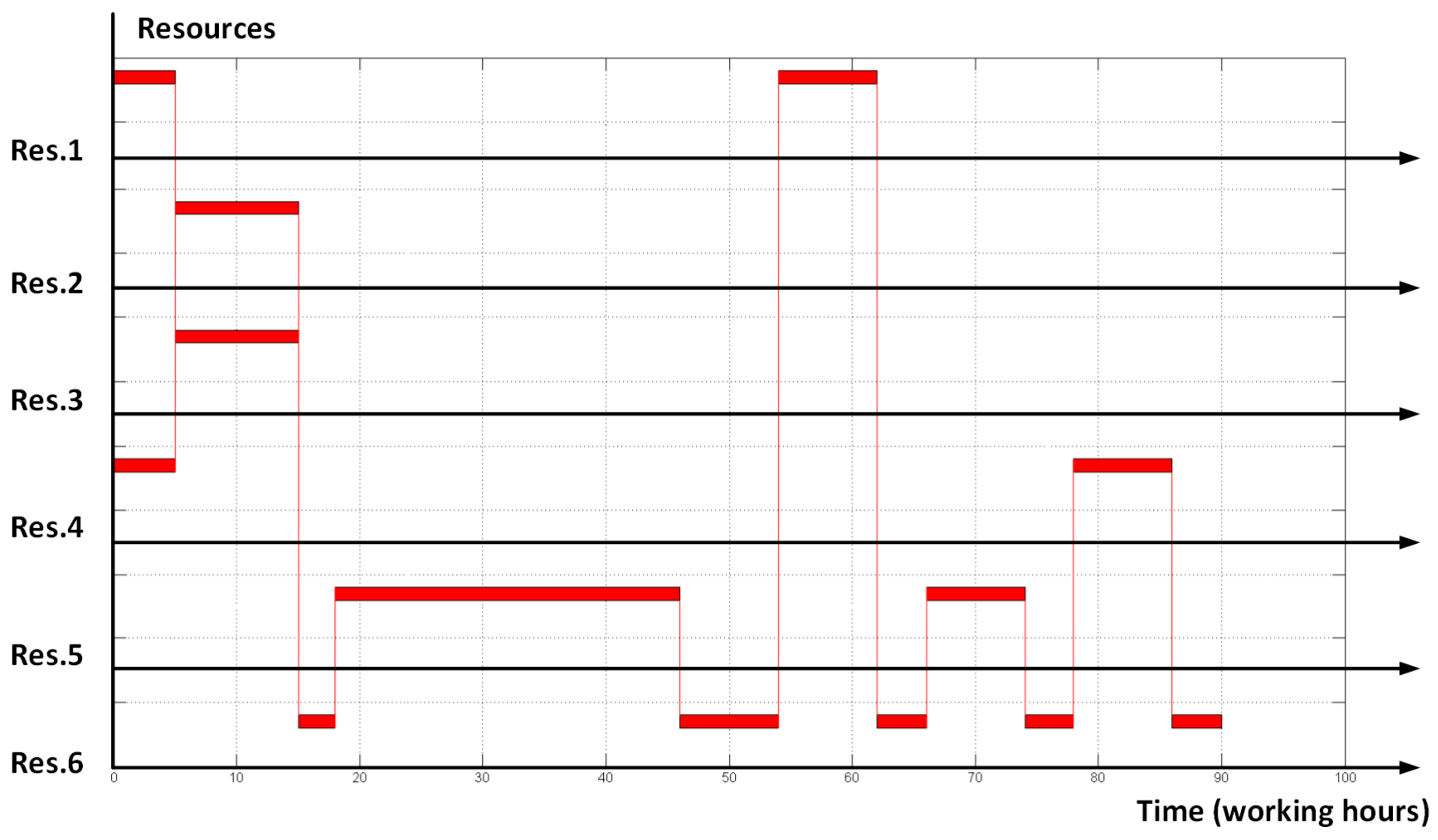
Figure 6.
Gannt diagram for starting point of two orders schedule optimization.
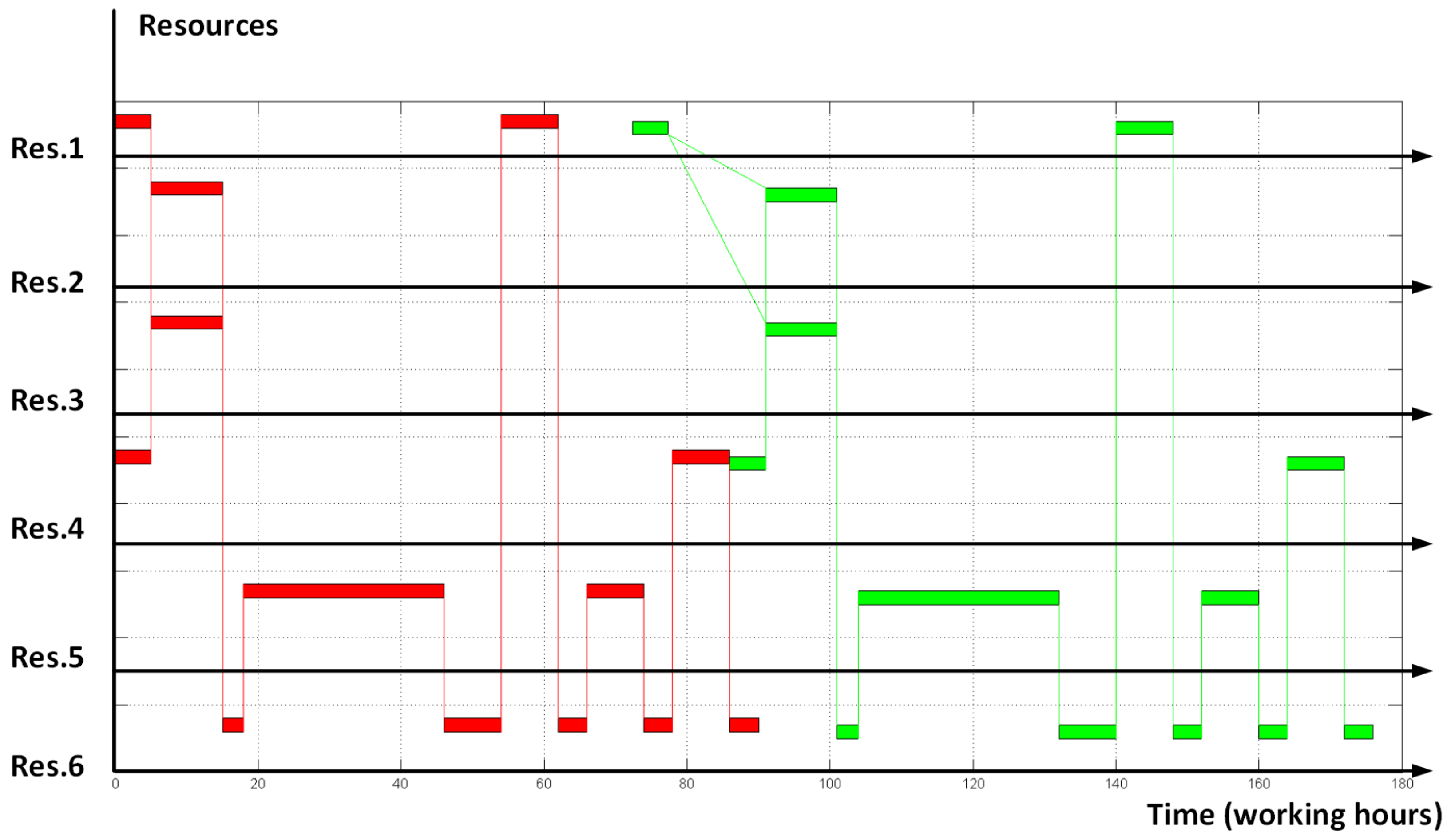
Figure 7.
Branch-and-bound optimization result.

Figure 8.
Gradient algorithm optimization result.

Table 1.
Algorithms test results: small number of operations (13 operations).
| Algorithm | Resulting “Makespan” Objective Function | Times of Orders Finished | Full Number of Operations Permutations (Including Non-Feasible) | Number of Iterated Permutations | Number of Iterated Non-Feasible Permutations | Calculation Time, Seconds | |
|---|---|---|---|---|---|---|---|
| Order 1 | Order 2 | ||||||
| B&B | 235 | 86 | 149 | 318 | 25 | 11 | 3.6 |
| gradient | 238 | 91 | 147 | 318 | 18 | 4 | 2.8 |
Table 2.
Results for 2 orders with number of operations increasing.
| Number of Operations | Algorithm | Resulting “Makespan” Objective Function | Times of Orders Finished | Number of Iterated Permutations | Number of Iterated Non-Feasible Permutations | Calculation Time, Seconds | |
|---|---|---|---|---|---|---|---|
| Order 1 | Order 2 | ||||||
| 25 | B&B | 348 | 134 | 214 | 71 | 29 | 5.4 |
| gradient | 358 | 139 | 219 | 36 | 9 | 3.1 | |
| 50 | B&B | 913 | 386 | 527 | 201 | 59 | 25 |
| gradient | 944 | 386 | 558 | 84 | 22 | 3.7 | |
| 65 | B&B | 1234 | 488 | 746 | 490 | 70 | 112 |
| gradient | 1296 | 469 | 826 | 126 | 66 | 11.2 | |
| 100 | B&B | 1735 | 656 | 1079 | 809 | 228 | 288 |
| gradient | 1761 | 669 | 1092 | 677 | 83 | 237 | |
Table 3.
Algorithms test results: increased number of operations (500 operations).
| Algorithm | Resulting “Makespan” Objective Function | Times of Orders Finished | Full Number of Operations Permutations (Including Non-Feasible) | Number of Iterated Permutations | Number of Iterated Non-Feasible Permutations | Calculation Time, Seconds | |
|---|---|---|---|---|---|---|---|
| Order 1 | Order 2 | ||||||
| B&B | 4909 | 1886 | 3023 | Unknown | ≈1200 (Manually stopped) | Unknown (≈10% of total) | Manually stopped after ≈7 h |
| Gradient | 4944 | 1888 | 3056 | Unknown | ≈550 | Unknown (≈30% of total) | ≈3 h |
| Random (gradient extension) | Trying implementing randomized algorithm led to high computation load of PC with no reasonable estimation of calculation time. Time to start first gradient iteration from feasible point took enumeration of more than 1000 variants. | ||||||
© 2018 by the authors. Licensee MDPI, Basel, Switzerland. This article is an open access article distributed under the terms and conditions of the Creative Commons Attribution (CC BY) license (http://creativecommons.org/licenses/by/4.0/).
Share and Cite
MDPI and ACS Style
Lazarev, A.A.; Nekrasov, I.; Pravdivets, N. Evaluating Typical Algorithms of Combinatorial Optimization to Solve Continuous-Time Based Scheduling Problem. Algorithms 2018, 11, 50. https://doi.org/10.3390/a11040050
AMA Style
Lazarev AA, Nekrasov I, Pravdivets N. Evaluating Typical Algorithms of Combinatorial Optimization to Solve Continuous-Time Based Scheduling Problem. Algorithms. 2018; 11(4):50. https://doi.org/10.3390/a11040050
Chicago/Turabian StyleLazarev, Alexander A., Ivan Nekrasov, and Nikolay Pravdivets. 2018. "Evaluating Typical Algorithms of Combinatorial Optimization to Solve Continuous-Time Based Scheduling Problem" Algorithms 11, no. 4: 50. https://doi.org/10.3390/a11040050
Note that from the first issue of 2016, this journal uses article numbers instead of page numbers. See further details here.