1. Introduction
The benefits of free markets derive from their “efficiency”, i.e., the idea that efficient markets accurately and rapidly impound new information into prices via trading. Market efficiency implies no information remains to be impounded in the price, hence, all new information is a surprise and is inherently unpredictable. Price movements in efficient markets are random, and consequently, conditioning on current and past information, reliance on prediction algorithms is futile. Our goal in this paper is to extend extant tests of market efficiency based on simple statistics to models based on deep learning neural networks.
There is a long history of research on market efficiency, beginning with [
1]. In a follow up article more than three decades later, Fama [
2] revisited the evidence on market efficiency, and found in favor of its broad existence using effective methods, especially event studies. These ideas have existed in the finance literature for a few decades. More recently, there has been a machine-learning-based literature [
3,
4,
5,
6,
7,
8,
9,
10,
11,
12,
13] that has also explored market prediction with some success, though the jury is still out on whether markets are inefficient and easy to beat.
Tests of market efficiency take many forms, such as tests of autocorrelation on univariate time series stock (or stock index) return data, as in [
14]. These tests of the weak-form market efficiency hypothesis take a narrow view of the information set on which the tests are conditioned, i.e., the history of the time series being predicted. Event study tests, beginning with [
15] also use information from the same time series, and complement this data with the return on the market index. These tests in general, also seem to support overall market efficiency, though of course, some anomalies do exist in the short-term. Tied up with an assessment of affirmative market efficiency is a corresponding proposition of an absence of stock predictability. In this paper, we revisit whether markets are predictable, in particular, if the direction of the broad market, not just one stock, might be predicted with higher than random chance.
Our approach, unlike existing methodologies, considers all stocks of the index and employs deep learning schemes to investigate market unpredictability. Two clear differences with existing approaches may be highlighted.
First, whereas weak-form tests have relied upon the history of a single time series of returns, we will assess the predictability of the daily direction of S&P 500 index using historical data on
all stocks in the index for a preceding period. Therefore, this is a large-scale generalization of the information set used in testing market efficiency. More complex techniques other than standard statistical ones have also been used where predictability surrounding turbulent market events is detected, see [
7]. Such approaches still use single time series for prediction and may not work well in normal periods.
Second, models for market efficiency tests have usually been based on linear statistical specifications, such as multivariate regression. Here, we will use highly nonlinear deep neural networks to specify the functional relation between the sign of the move in the S&P 500 on day and the T-day history of all stocks in the index until day t. The hope is that what linear models cannot pick up, we may train nonlinear models to learn. Furthermore, by expanding the information set by a huge order of magnitude, we are able to re-examine weak form efficiency more comprehensively. Using the expanded information set, we find that deep learning approaches, with their nonlinear structures do better than a panoply of other comparison prediction algorithms, though not well enough to reject a finding of market efficiency.
Market efficiency, evidence by a lack of predictability is usually supported by two features of the data. First, randomness. A purely random series is, by definition, unpredictable. Second, nonstationarity. This belies predictability because the fitted parameters from historical data have limited shelf-life, and become invalid in forecasting the future evolution of returns. Our results are two-fold. First, we find that predictability of the S&P return using all 500 stocks in the index exists, but is weak, and too small to be profitable after taking transactions costs into account. Second, we find evidence that both randomness and non-stationarity make prediction difficult, but randomness plays a bigger role in making markets efficient.
One may argue that tests of market efficiency that assess whether mutual funds can beat the market (see [
16]) are in effect using much larger conditioning datasets than single stock series. Once again of course, these are time series tests with a single series of the fund at a given point in time. In addition, these tests are linear, and do not admit nonlinearity in their specifications. Therefore, we believe that the use of deep learning neural nets to develop a stock index predictability model are novel, and despite the long history of empirical support for market efficiency, such models, in theory, may be using information sets in a different way, one that has not been assessed before. Whereas it may be quite impossible for a human to detect predictive patterns in reams of stock data, it may be within the realm of possibility for machine intelligence. In addition, though the S&P index seems only weakly predictable, other asset classes, such as small stocks, may prove to be less efficient in the face of large information sets.
In the following sections, we explore this new approach to testing market efficiency.
Section 2 recaps the architecture of neural nets, including a discussion of the backpropagation technique.
Section 3 describes the data engineering used in this paper, and has some interesting ways in which we handle the data in order to render it suitable for consumption by a deep learning model.
Section 4 describes the experimental structure used, and
Section 5 describes the results.
Section 6 provides concluding discussion.
2. Neural Networks
Neural networks (NNs), the primary methodological tool used in our analysis, have been in existence since the 1940s, beginning with the early work of [
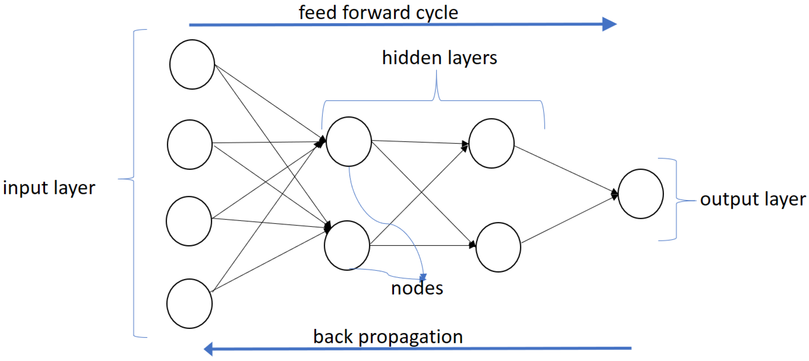
17], but have become immensely popular in the last decade due to dramatic increases in computing power and the explosion of available data. NNs are set up to imitate the decision-making process of the human brain. An example of a neural network is shown in
Figure 1. This network has four layers: an input layer, two hidden layers, and an output layer.
However, the simplest exemplar of a neural network is a single perceptron. A typical perceptron is implemented using the “sigmoid” function, also known as the “output activation” function.
where
a is called the “neuron input” to the sigmoid function, and is a weighted sum of outputs from the preceding layer. There are several different types of neurons and another popular one that we use in this paper is known as the “restricted linear unit” or ReLU for short. This has a piecewise linear functional form.
Therefore, this neuron emits an output of zero, unless its input a is positive, in which case it emits a.
The first layer with input values (usually denoted x) is called the input layer, the middle layers with function values (usually denoted y) are called the hidden layers and the last layer with z values is called the output layer. The functions at each node are called “activation” functions, borrowing from neuroscience terminology where neurons are said to fire or activate. There may be several hidden layers and multiple perceptrons (nodes) in each hidden layer. Neural nets with multiple layers (sometimes more than 100 layers) have resulted in the nomenclature of “deep learning” neural nets. Higher number of layers or nodes naturally lead to longer processing times. The output layer can either have multiple outputs or a single output (binary classifier). In the case of a binary output, the output layer is implemented with squashing functions that emit an output value between 0 and 1. The neural network we use in our paper is a fully connected feed-forward network, i.e., each input layer node is connected to each node in the first hidden layer. Each node in the first hidden layer is connected to every node in the subsequent layer, and so on, till we reach the output node(s).
For our stock prediction algorithm, we would inject the information set (in our case, data histories on all stocks in the index) into the (left side) of the neural network. Each layer in the network comprises nodes, i.e., a set of mathematical functions that transform the data, which is then fed into the nodes (functions) in the next layer, until finally the output layer is reached. The output function in our case generates a value in the interval , i.e., the probability that the market will go up in the forecast period. Intuitively, the neural network is a giant nonlinear function that takes in a large number of inputs and generates a prediction about the likelihood that the market will rise in the ensuing period.
2.1. Working of a Neural Network
The easiest way to understand how a neural network works is to note that each of the inputs (the x values) are provided as weighted inputs for the first hidden layer, and the outputs of the hidden layer become the inputs to each subsequent hidden layer. The weights vary for each node in every hidden layer and the output layer.
In our example in
Figure 1, the inputs
x are passed to the first hidden layer
y, and at each node in the first hidden layer, the inputs are weighted to arrive at what is called the “neuron input”. So for the network shown in
Figure 1, there are two nodes in the hidden layer and the neuron input for each node is as follows, given the four input values
.
where
are the two neuron input values, and the weights are
, which are the parameters of the model that need to be calibrated. The constant terms
are the “bias” terms and cause a linear shift of the neuron input value. The superscripts denote the number of the hidden layer; here “
” denotes the first hidden layer. The first hidden layer has ten parameters (eight
w values and the two bias
b values). The second hidden layer has six parameters. Each node of the two hidden layers generates a single output through a nonlinear transformation of the neuron input, i.e., if we use sigmoid functions, then these would be as follows.
These values are then passed to the second hidden layer, with its own neurons that emit values into the final output layer, where the single sigmoid neuron produces a value between 0 and 1. This model example in
Figure 1 has 19 parameters or weights, five for each node in the first hidden layer, three for each node in the second hidden layer, and three for the output node. In a typical deep neural network with several layers and many nodes per layer, the number of parameters can be much larger, hundreds of thousands to the low millions.
The weights , for all , and all hidden layers r, are chosen to minimize the prediction error of the neural network on training data. The error is combined into a loss function across all or subsamples (known as batches) of the training data, usually by choosing the loss function to be the sum of squared prediction error, or some other loss function such as entropy. The calibrated weights will determine the accuracy of the network in predicting the output, i.e., the movement of the S&P index in our tests of market efficiency.
The biggest challenge in calibrating an accurate neural network, is calculating the weights to be used at each layer. Today this challenge has been surmounted by special purpose hardware, and commoditized programming tools, such as Google’s TensorFlow (
https://www.tensorflow.org/) and other popular open source implementations of neural networks such as MXNet (
http://mxnet.io/), and h2o (
https://www.h2o.ai/). In conjunction with better hardware and software, one single mathematical innovation from more than three decades ago is solely responsible for the incredible efficacy of deep learning neural networks—backpropagation, often shortened to “BackProp.”
2.2. Calibration via Backpropagation
We may think of the neural network as a large-scale function approximation, where the network is calibrated (using the inputs) to best fit the true output as closely as possible. Therefore, calibrating a neural network involves optimization, where a loss function
is minimized, by choosing the weights
and bias terms
of the model as best as possible. Finding the best parameters by minimizing the loss function provides a best effort result at uncovering a function that approximates the mapping from inputs to outputs. Because neural net architectures can be as large and complex as the modeler likes, these nonlinear functions are often called “universal approximators”—they can approximate any function. Our goal is to find the best prediction function that approximates how the history of stocks’ returns determines the future direction of the stock index. This goal is supported by the Universal Approximation Theorem, which asserts that a neural net with a single hidden layer, a large number of nodes, with continuous, bounded, and non-constant activation functions can approximate any function arbitrarily closely ([
18]), though this has been debated by [
19].
Optimization is undertaken by adjusting the parameters in the model by moving each parameter in the direction that reduces the loss function, at a speed known as the “learning rate.” This direction is given by the gradients of the loss function
,
with respect to the weights. This fitting approach is known as “gradient descent”. Given the large number of parameters in the huge neural nets in vogue today, gradient computation must be efficient. Preferably, it should be analytical. The backpropagation algorithm does exactly that, i.e., it provides an analytical scheme for calculating all gradients. The evolution of the backpropagation algorithm covers the past 50 years, through seminal work by [
20,
21,
22,
23], the latter being the implementation that is widely used. (For an accessible, technical introduction to neural nets, see (
http://srdas.github.io/DLBook). Excellent books on the subject are by [
24,
25]. An online resource is Michael Nielsen’s book: (
http://neuralnetworksanddeeplearning.com/.)
We move on now to discuss the data used in our prediction experiment to test for market efficiency.
3. Data Engineering
3.1. Sourcing and Formatting the Data
The primary source of data is the daily returns of the S&P index and its underlying stocks extracted from the Wharton Research Data Services (WRDS) database, from April 1963 to December 2016. This gives us approximately 54 years of daily return data for our analysis, across thousands of stocks. Note that there are many tickers involved as they move in and out of the index.
We built the data for the daily returns of the component stocks as follows. Using the Compustat database a query was run to collect all tickers of the S&P 500 between April 1963 and December 2016. The unique identifiers from the resulting file were then run against the WRDS database to collect historical security prices for all the securities in the time period of our analysis. (Both Compustat and stock data come from the Wharton Research Data Services (WRDS) platform. See: (
https://wrds-web.wharton.upenn.edu/wrds/.) Stock prices are converted into returns, implicitly implementing data normalization, which also makes the data comparable across all stocks in the sample.
Daily returns of all component stocks that were a part of the S&P 500 index between April 1963 and December 2016 are collected in a table with dates on the rows and stocks on the columns. Since there are many additions and deletions of stocks from the index, we end up with 5370 different stock tickers over the sample period, and these account for several additions to, and deletions from, the index, over a period of 54 years (13,532 trading days) covered by our sample. This data matrix contains many missing values, as only 500 stocks at a time exist in the index, and is therefore a semi-sparse data matrix. The degree of sparsity is 68.54%. We also counted the proportion of days on which the index rose (versus fell), which is
of the time. All told, we have a daily return matrix comprising 13,532 rows and 5372 columns (noting that one of the columns is for dates and the remaining for stocks, and the index). See
Figure 2 for a depiction of the stock price and return data. Note that the price and return matrix is sparse as all stocks did not trade on all dates.
3.2. Feature Engineering
We face two issues with the data matrix. One, there are missing values. Since over the past 54 years many stocks have entered and exited the S&P 500 index, we had to account for the fact that a security would have influenced the movement of the index only during a certain period. Also, even for just the L-day history in the feature set, some columns may have missing data as stocks may have left the index and others may have entered it. Two, if we use all 500 stocks’ returns for a day and we have a look back period of days, then our feature set will have 15,000 variables and the training sample will only be of size or (the two training sample lengths we experimented with). Both these issues are resolved by reducing the dimension of the feature set.
Our remediation entails using only a few return percentiles each day, which results in a drastic reduction in dimension of the feature set. We convert the daily returns of the 500 underlying component stocks to
percentiles. The percentiles considered are at the 1, 2, 3, 5, 10, 15, 20, 30, 40, 50, 60, 70, 80, 85, 90, 95, 97, 98, and 99 percentile levels. This results in a dataset that has the sign of the daily return (direction) of the S&P as the (binary) dependent variable, and 19 percentiles as the explanatory variables per day, thereby reducing daily data dimension from 500 to 19. These percentiles allow us to capture the entire distribution through a discrete approximation, and places each day’s data into a standard data structure for the probability distribution of returns. This reorganization of the data allows us to abstract from the fact that the underlying stocks in the index are changing, yet considers the influence of their returns in predicting the forward movement of the S&P. It allows modeling the return of the index based on all its 500 component stocks at any point in time, reduced to a summarized set of
values. It also results in a tidier dataset for the prediction exercise that is the focus of our analysis. In addition, there are no missing values in the transformed data matrix. With a look back period of 30 days, for example, each row of the dataset now has size 570 (
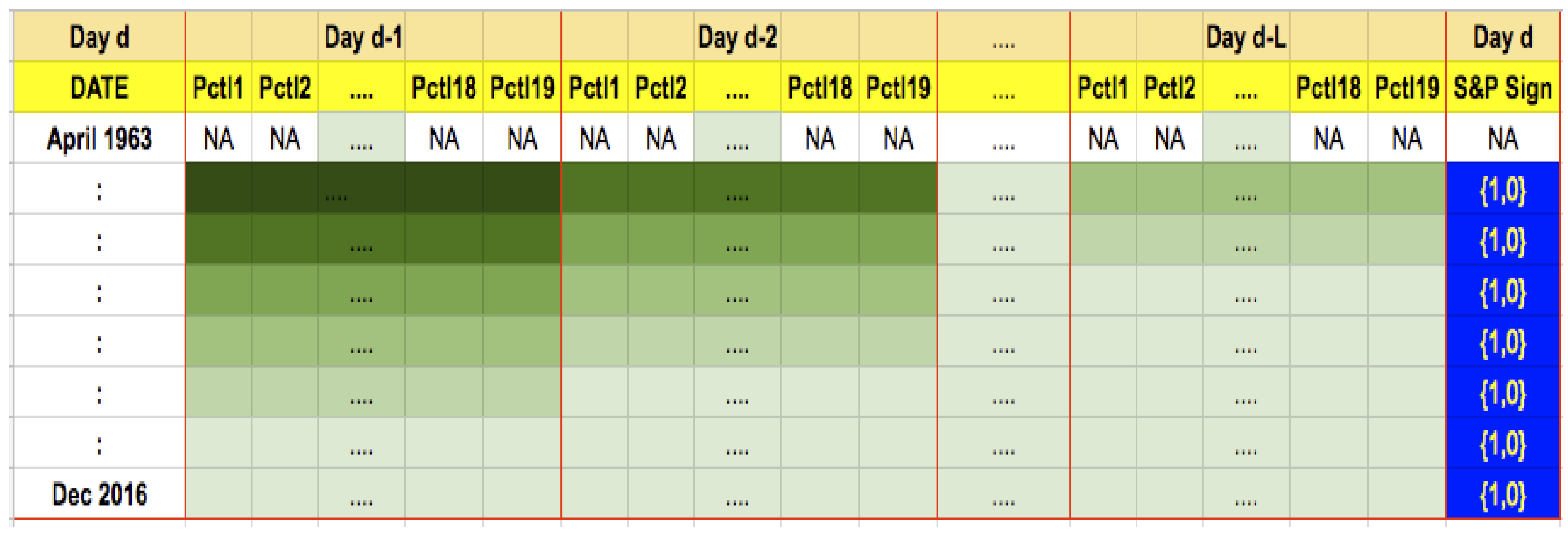
) values of stock return percentiles. The dataset is no longer sparse and is shown in
Figure 3.
More formally, as shown in
Figure 4, this feature creation essentially lines up
L days of stock return history from day
back to day
, placed side by side in the same row for a given date. Therefore, there will be a block of columns for
, another block for day
, and so on, until a final block of columns for day
, each column representing one of
C stock return percentiles for one of the
L preceding days. Therefore, the size of the data input for training the algorithm is
N rows of
features. The corresponding training labels will be a single column of values, which are 1 if the index moved up on date
t, else zero.
3.3. Statistical Features of the Dataset
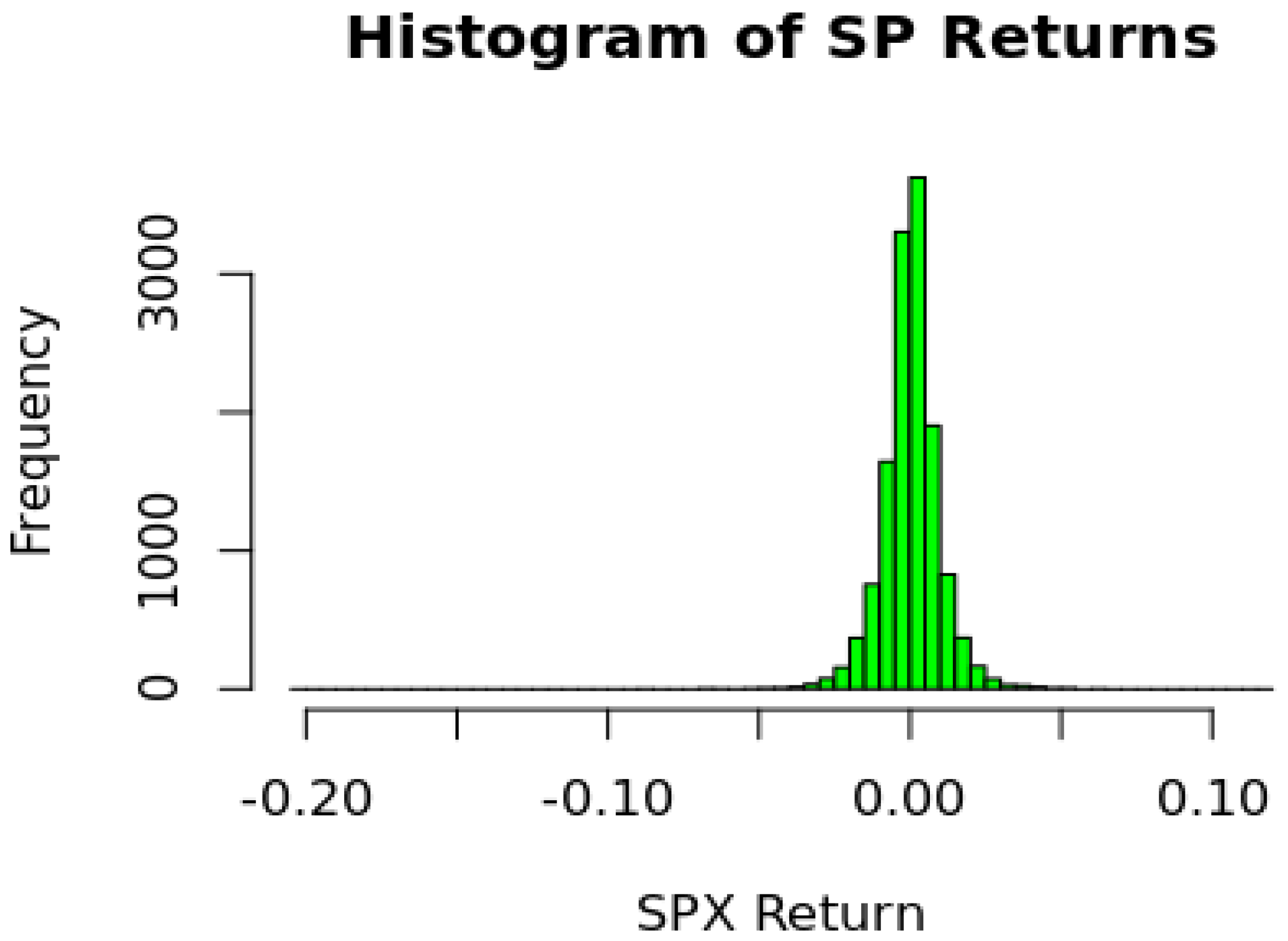
We begin by reviewing some attributes of the data. The distribution of the S&P returns is shown in
Figure 5. As seen from the histogram returns are tightly distributed with most of the daily returns between
and
. The distribution has mild negative skewness and high kurtosis, both known features of index return data.
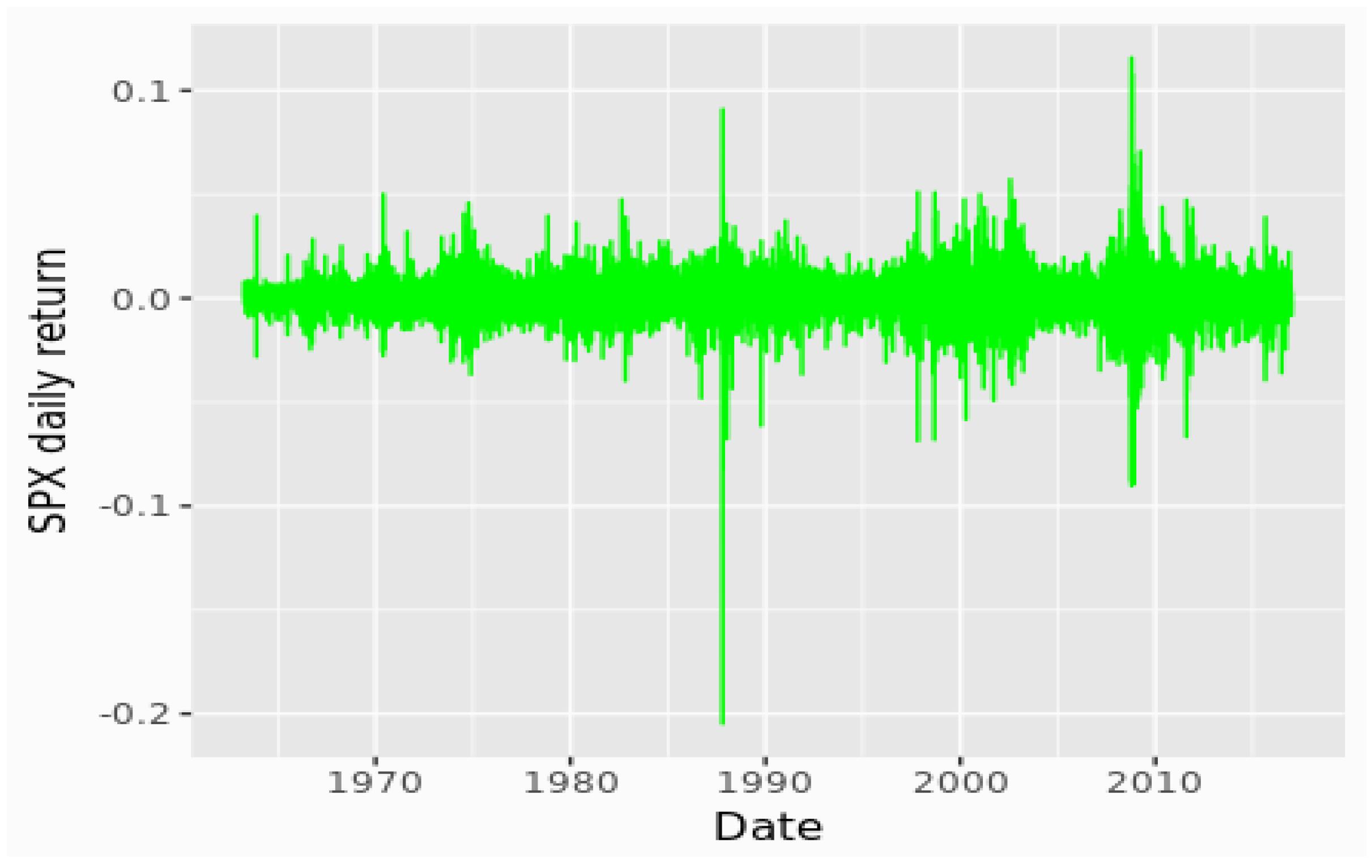
A plot of the daily returns, shown in
Figure 6, confirms the presence of large outliers, leading to kurtosis, and periods of high and low volatility.
4. Experiments
This section details the structure of our empirical analyses. We describe how we partition the data for training and validation, how we set up rolling periods, the structure of the deep neural net, and the metrics we use to assess prediction performance.
4.1. Look Back Period (L) and Prediction Function (M)
We use the data structure we created as described above to forecast the direction of movement
in the S&P 500 index for any given day
d as a function of data over a look back period of
L days, i.e., over a set of days
. The number of days of data used for training is
N (not to be confused with the look back period
L defined earlier in
Section 3, and here in this section). Therefore, we may think of the fitted deep learning model (
) as the following function:
That is, we pass into the function the last
L days of data to predict the movement on the next day, or subsequent days. For each day in the
L-day history, we may have
C columns of data. In our experiments,
, and these are percentiles of the return distribution for the 500 stocks in the index. Thus, the model uses
inputs to generate a binary classification
M. For training purposes,
N such inputs will be used, i.e.,
N rows of features, each of size
. We note that
. The dataset is depicted in
Figure 4.
4.2. Forecast Period (F)
After fitting the deep learning model, we then hold the model fixed and use it to forecast index direction over an out-of-sample forecast period (F), i.e., for days . We then compute the accuracy of our prediction, i.e., the percentage of days in the forecast period F for which the model was able to correctly predict the sign of movement of the index.
4.3. Training Set Size (N)
N is the number of observations used to train the model. This is a sliding window, and each forward forecasted period F is modeled on the previous N observations. For our analysis we have considered , each forecast period F is predicted based on a training set of the previous N days, each day’s observation consisting of a look back period of L days.
We train repeated models on a rolling basis, each with N data observations. Each row of these N observations contains days of history. Even though we use preceding periods’ data to predict the index move for the forecast period, our data structure does not require it, as each row in the dataset contains the target variable and all the preceding days’ data that is needed. However, note that the structure of the feature set retains the time sequence of the data. The advantage is that we may sample data randomly as well from the entire dataset when constructing training and validation samples.
L is the look back period, the number of previous days’ percentiles which have been considered in predicting the next day’s S&P return. For example, if , that means today’s return was considered to be dependent on the previous 30 days’ percentiles of the underlying stocks. In our analysis we consider various forward forecast periods (F) of 10, 30, 1000, and 5000 days. The combination of L and F results in multiple sets of parameter choices for our prediction experiment.
4.4. Training and Validation
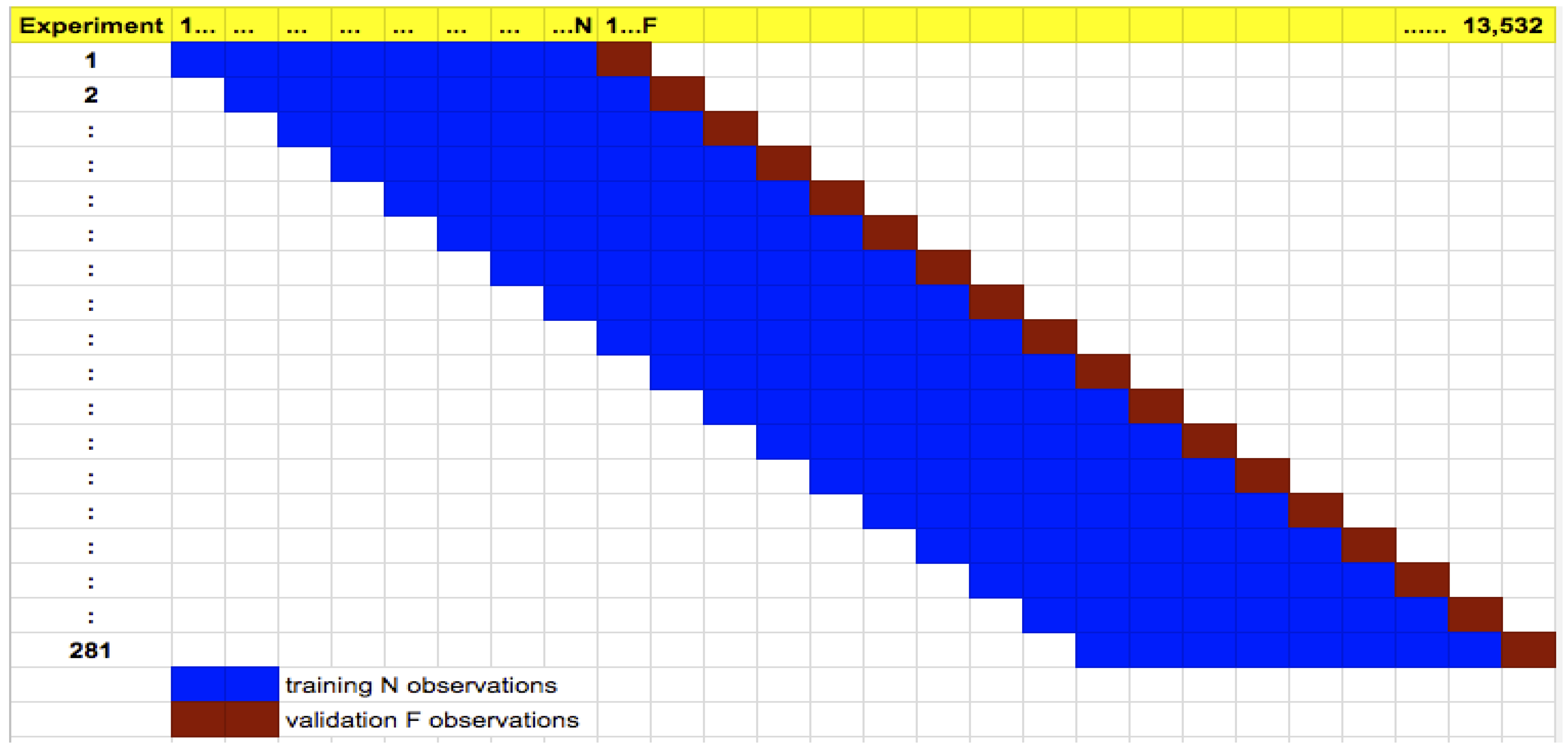
We perform repeated training and validation using rolling period samples. Our training set size is
and each row in the training data comprises data from
days. After training our deep learning net, we then forecast the next
days market direction. We then roll the sample
F days forward and repeat this experiment. Altogether, depending on the value of
F, we have different numbers of experiments. For example, when
, we conduct 422 experiments across the entire time series of the dataset (think of this as 422-fold cross validation). The general scheme is shown in
Figure 7. Training for each experiment across all rolling cases takes about 3 h, with 6 CPU and 25 GB assigned to the
h2o cluster. Therefore, each episode of training and test takes less than 30 s.
Unlike cross-sectional data, our time series dataset lends itself better to rolling training and validation where the training period always must precede the validation period. Hence, there is no need to keep a hold-out test sample. For each experiment we report various test statistics: precision, recall, F1 score, area under the curve (AUC), and root mean squared error (RMSE). Because we have many experiments, we are in a position to report the distribution of these statistics generated from experiments spanning more than 5 decades (1963–2016). Therefore, we get a pretty good idea of whether deep learning neural nets reveal market inefficiency.
4.5. Prediction Models
We model the direction of returns as binary. We consider any day where the daily return is positive as having a value of 1, and any day when the return was negative or zero is given a value of 0. Our implementation attempts to predict the direction of the movement, rather than the magnitude of the movement itself.
We fit a deep learning neural net model to the data. The model has the following structure, i.e., hyperparameters. The input layer comprises
inputs. The number of hidden layers is 3 and each layer contains 200 nodes. The activation function used is Rectifier (i.e., Rectified Linear Unit (ReLU) functions) with Dropout (dropout rate of 20%), Batch Gradient Descent is used, and a crossentropy loss function with 50 epochs of training. The model is implemented in the
R programming language using the deep learning package from
h2o.ai. (See
http://h2o.ai). Nesterov accelerated gradient descent is applied with mini batch size equal to 1 by default (i.e., online stochastic gradient descent). We also implemented the model using TensorFlow using Python, and obtained similar results.) The model is a fully connected, feed-forward network with no CNN (convolutional neural net) or RNN (recurrent neural net) features. Standard backpropagation is applied.
We model various scenarios, in each case using observations to train our model and building a model with a 30, 60, and 90 look back period and a forward forecast of 10 and 30 days. We report the results for the case, as this is not dissimilar to the cases. As the prediction period F increases, the accuracy of the model decreases. We report the results for the days case.
4.6. Prediction Performance
We measure accuracy in various ways:
Forecast period average accuracy (FPAA): In this measure we calculate the ratio of the number of days per forecast period that our model predicts the index movement correctly (i.e., accurately predicts that the index went up when it actually went up and vice versa) to the total number of forecast period observations. Next, we take the ratio of the number of periods that our model was over 50% accurate to the total number of forecast periods. For example, suppose over three forecast periods our model was accurate 60%, 60% and 30% of the time. Then, the FPAA would be 66.66%, as our model predicted over 50% accuracy twice in the three forecast periods. This measure gives us a point in time measure of how our model is performing and is labeled as average accuracy in each of the runs discussed below. The measure indicates whether identical trades over the forecast period F will lead to a gain on average. The FPAA measure is a new measure that we developed for this paper.
Overall accuracy (OA): In this measure we focus on the daily measures of accuracy. We take individual day level predictions and compare it to the actuals to generate a confusion matrix for each experiment, from which we calculate accuracy. This measure of accuracy gives us a rolling historical measure of the performance of our model. This measure is the number of correctly predicted days across all days in all experiments.
Precision, Recall, F1, AUC: These are standard measures for prediction algorithms based on a binary confusion matrix. We recap these here, where is the number of true positives; is false positives; is true negatives; and is false negatives. Precision is ; Recall is ; and is the harmonic mean of precision and recall, i.e., . The area under the ROC curve (AUC) measures the tradeoff between the false positive rate () and the true positive rate (). AUC is one of the most comprehensive measures of prediction performance.
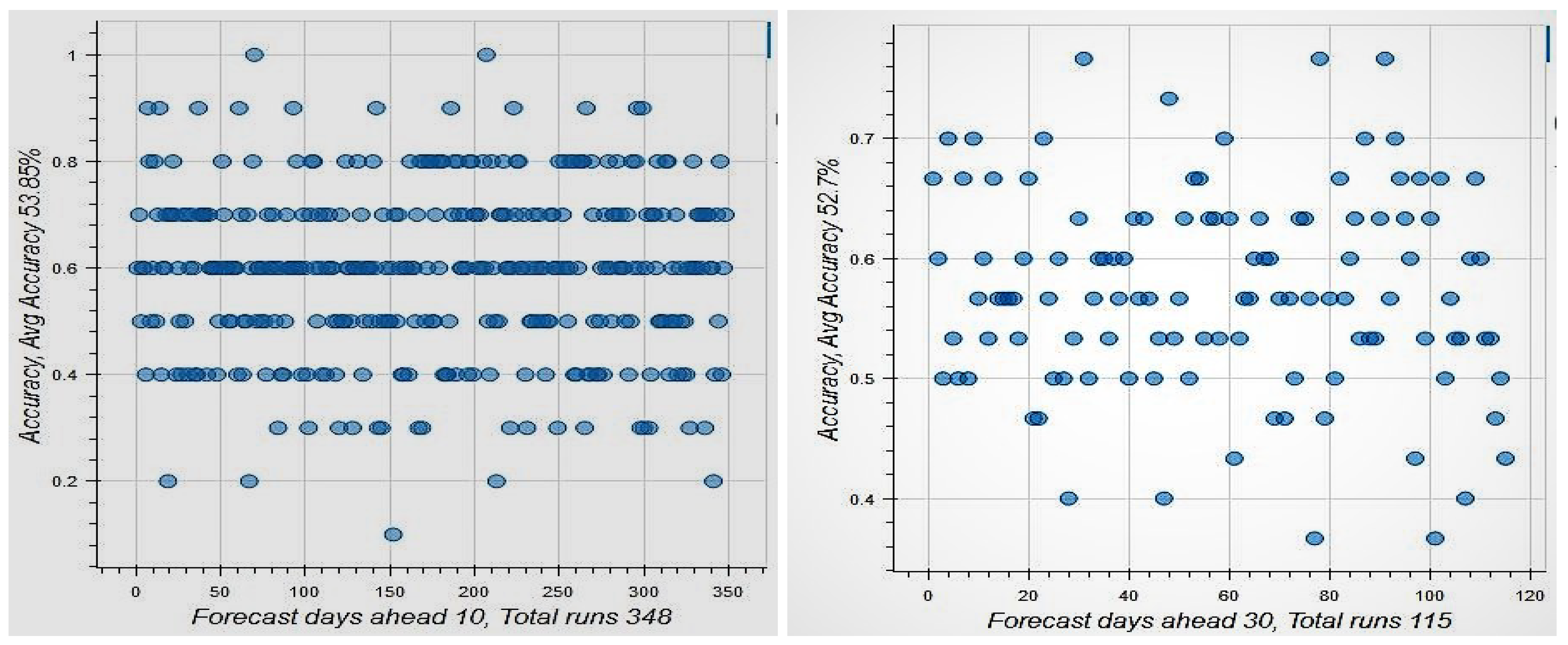
Figure 8 shows the results for the case when the look back period is 30 days and the forecast period is either 10 or 30 days. In the former we obtain many more non-overlapping rolling periods. This results in 348 non-overlapping forecast periods for
, and 115 non-overlapping periods for
. Forecast period average accuracy is 64% for
days and 77% for
days. Even when we check how many blocks we had accuracy greater than 52.7%, we arrive at the same forecast period average accuracy of 77%. both well over 50% as can be seen from the number of points in
Figure 8 that lie above the
level on the y-axis. The OA is slightly over 50%, i.e., 53.9% for
days and 52.7% for
days. Given that the percentage of days that the market went up in the sample is 52.7%, this suggests very weak predictability. Hence, using short-term forecasts, we see that markets are efficient when conditioned on the information in large datasets and modern deep learning tools. Even if the forecast period accuracy were exploitable in some way, the levels of accuracy are average but may not be enough (especially after transactions costs) to suggest that market efficiency may not be supported when a larger universe of information is considered in modified weak-form efficiency tests.
4.7. Identifying the Sources of Market Efficiency
Given that our evidence suggests that markets are more or less efficient, we may proceed to use the technology we have to uncover whether the lack of predictability comes from one of two possible sources; (i) random movements in the stock index, or (ii) nonstationarity in the distribution of stock index returns. In this section, we describe a non-parametric approach to ascribing the lack of predictability to each of these sources.
We set the lookback period to days and the forecast period to days. The size of the training data (rows of data) will be . We also fix the number of epochs in the fitting exercise to be 50 as before. We compute OA from the following three experiments.
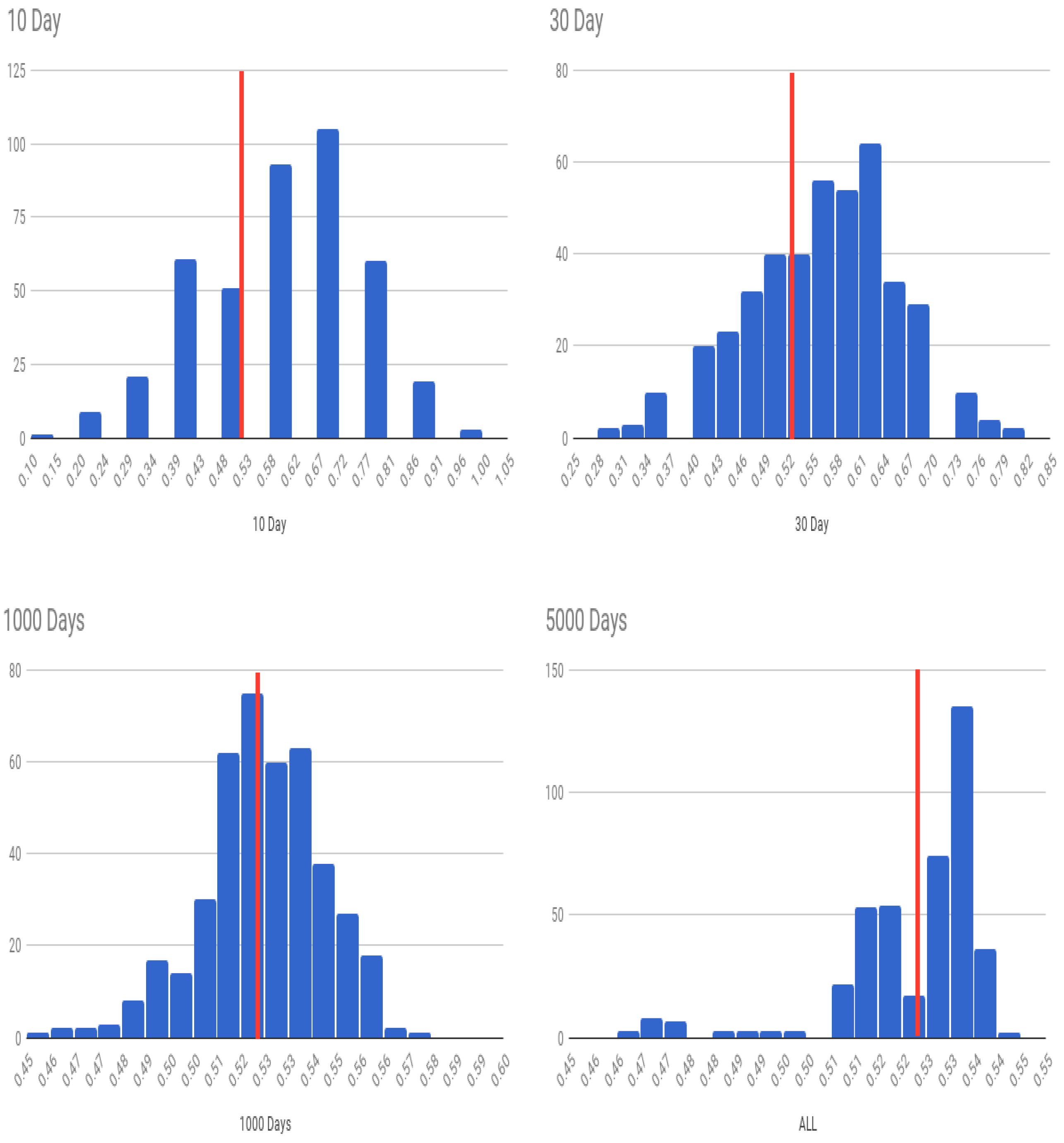
In-sample: Using 5000 observations, starting from the first day of the sample, we train the neural net, and then test it on three sets: (i) a randomly chosen set of 10 observations from the training sample; (ii) a randomly chosen set of 30 observations from the training sample; (iii) a randomly chosen set of 1000 observations from the training sample; and (iv) the entire training sample is treated as the test sample. We then roll forward 20 days and repeat this experiment. This will give us 423 such experiments, each with four accuracy values (one from each test set) for “OA” and for “FPAA”.
Stationary out-of-sample: Here we try to maintain stationarity in the sample by bifurcating the sample into separate training and test groups but from the same sample period using a block of consecutive 5000 observations. (i) Randomly select 4990 observations for training and keep the remaining 10 for testing; (ii) randomly select 4970 observations for training and keep the remaining 30 for testing; (iii) randomly select 4000 observations for training and keep the remaining 1000 for testing. as in the previous case, roll forward 20 days and repeat this experiment.
Nonstationary out-of-sample: Starting from the first observation, pick a block of consecutive 5000 observations, and train the deep learning model. Then, (i) test the model on the next 10 observations; (ii) test the model on the next 30 observations; (iii) test the model on the next 1000 observations. Roll forward 20 days and repeat this experiment.
Each of these experiments gives an “OA” that is denoted where for each of the classes above. By comparing these cases, we can determine how much prediction error is supported by randomness versus lack of stationarity. In the following section, we quantify these accuracy values to determine the sources of lack of predictability.
5. Empirical Results
In this section, we denote the three cases as follows: in sample (IS), stationary out-of-sample (OS), and nonstationary out-of-sample (NS). For each of these cases we report the FPAA and the OA. The results are reported in
Table 1.
We first examine the four experiments we conducted in the IS case. The OA declines as we predict larger subsets of the data for testing, albeit in-period. However, the chance that we do better than a coin toss over forecast blocks (FPAA) keeps increasing. As the test dataset increases, since the algorithm already shows greater than 50% accuracy, the average likelihood that any prediction sample will be predicted more accurately than 50% naturally increases, as is expected. (When you have a biased coin with more heads than tails, the number of experiments in which heads will exceed tails will increase in the length of the number of coins tossed in each experiment.) Ultimately, if the test dataset is the same as the training data, the small level of predictability is amplified to deliver very high levels of average accuracy. The histograms of all experiments are shown in
Figure 9.
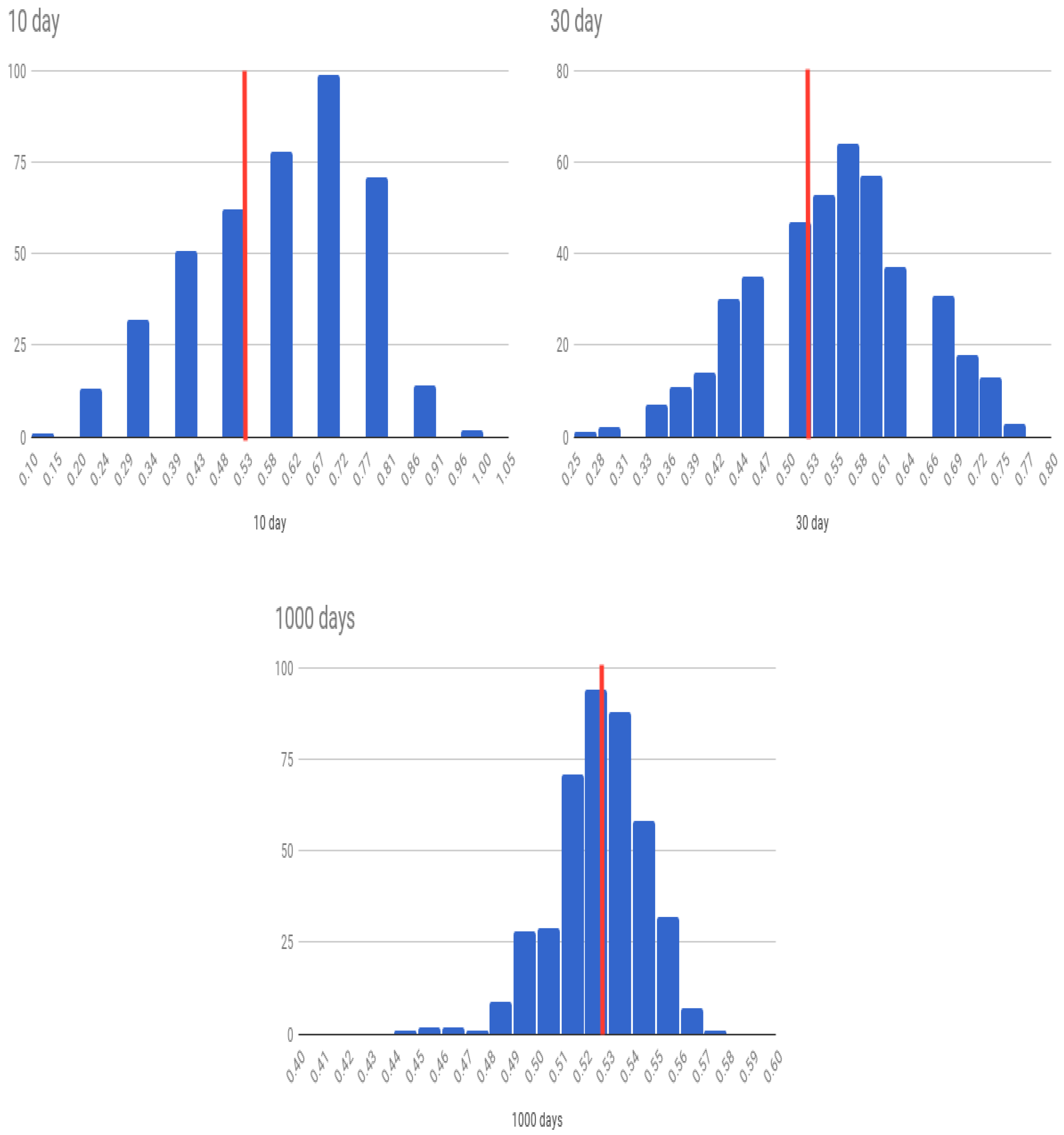
Next, we look at the case where we use OS values from within the same period, i.e., the stationary (OS) case. The histograms of all experiments for the OS case are shown in
Figure 10. The difference in accuracy between the IS and OS cases may be attributed to randomness because in both cases the training and the testing sample are drawn from within the same continuous period of time. In the third set of results for the nonstationary (NS) case, we see almost similar results to the stationary case. The histograms of all experiments for the NS case are shown in
Figure 11.
The patterns in
Table 1 show that OA declines as the forecast period lengthens for all three cases of forecast experiments. The baseline is the percentage of days for which the market moved up, which for the current data sample is
. The case of
days look-ahead quickly dissipates to the baseline level expected, as the forecast period is very large, and is to be expected if the market is efficient, which there is evidence of (in [
14]). Therefore, it is more interesting to examine how the OA declines as the forecast period is extended from 10 days to 30 days.
First, in all three experimental conditions, OA declines as we extend the forecast period from 10 to 30 days. This suggests that recent history does matter in prediction, and is also intuitive, as the joint statistical distribution of market stocks is likely to be stationary for small look-ahead windows. We examine this phenomenon for the OS case with additional granularity, taking the forecast period to be in the
days, results shown in
Table 2. The forecast accuracy declines (albeit slightly) as we increase the forecast period, confirming that a small amount of the loss of predictability may be attributed to nonstationarity.
Second, we see that the difference in prediction accuracy () between the IS case, stationary case, and nonstationary case is small for the case when days. The suggests that the lack of predictability here () comes from randomness and not nonstationarity.
Third, for the days case, the difference between the three cases is also small, but the difference between the IS case and the two OS cases is bigger than for the case. We may attribute this to the effect of nonstationarity.
Fourth, we see from the days case, that the OA has dropped back to the baseline of , as the full effect of nonstationarity and randomness erase all predictability.
Fifth, in both, the
cases, the accuracy level is higher than the baseline percentage number of days for which the market goes up (52.7%). Yet, it is hard to argue that the predictability is sufficient to generate low-risk profit after transactions costs. In fact, even ignoring transactions costs, note that in no case was the OA different from the baseline expected percentage of “up” days of 0.527 by more than 0.5 standard deviations, see
Table 1. Clearly, there is no statistically significant evidence of superior prediction ability. Hence, these experiments confirm, with large-scale testing, that markets are efficient for an investigation of predictability of the S&P 500 index.
Sixth, the verdict that markets are efficient (for a test of broad index prediction as undertaken here) is further supported by the poor results on other metrics such as precision, recall, AUC, and F1 scores. We see an imbalance where precision is average, but recall is very high. Therefore, the algorithm misses more down ticks in the market but captures most of the upticks. With such an algorithm, one would act aggressively on up signals and ignore most down signals. The low average AUC scores further confirm that markets are efficient.
In order to assess whether simpler techniques might in fact yield better results, we fit a logistic regression model to the dataset as well. In this case, we used observations for training, a look back period of days, and a forecast period of days, as this was the best case result for the deep learning net. Rather than rerun all cases, we only examined the OS nonstationary case (NS) as this is the one that is relevant for a practitioner trying to make money from predicting market direction. Here, (SD = 0.15), i.e., logistic regression has an accuracy level much worse than that of the neural net (OA = 0.582), though this is not statistically significant.
In addition to the logistic regression, we also ran six other prediction models using the same feature set and labels. These six models are: decision trees, random forest, linear discriminant analysis, k-nearest neighbors, naive Bayes, and support vector machines. These were all for the case of practical interest, i.e., the rolling OS test.
Table 3 reports the results for the deep learning net and all the other models for comparison. While deep learning does better than the other models, in no case is it possible to beat the market in a statistically significant manner.
6. Concluding Discussion
This paper offers a small experiment to assess the potential of deep learning algorithms to predict markets. Using data on all stocks on the S&P 500 index from 1963 to 2016, we train a fully connected, feed-forward deep learning network with three hidden layers of 200 nodes each to predict the direction of the S&P 500 index daily. Unlike existing tests of weak-form market efficiency, which use a single return series to test for autocorrelation, this new approach expands the information set by a huge order of magnitude, i.e., by using return data from all stocks in the index for the past 30 days. The trained prediction model is then used for look-ahead periods ranging from 10 to 30 days, and more.
Over the entire sample period, the percentage of days for which the S&P index moves up is 52.7%. Therefore, our prediction algorithm needs to predict up moves better than this percentage and not just do better than 50%. (Note that a naive algorithm that predicts markets always move up will be correct 52.7% of the time.) With look-ahead periods of 10 days (OS), we find that the model gets the predicted movement correct about 58% of the time. For a look-ahead period of 30 days the accuracy is 55%. While this is greater than 52.7%, it is not statistically strong enough to claim that deep learning is able to predict the markets. We may therefore conclude that our tests, which use vastly greater information sets than hitherto used in weak-form tests of market efficiency, do not uncover strong evidence of market inefficiency. However, the shapes of the histograms in
Figure 9,
Figure 10 and
Figure 11 suggest that the model is performing well as more of the density loads to the right of the average up-move percentage line. This visual depiction is also reflected in the FPAA metric shown in
Table 1. We conjecture that more tuning of the architecture may lead to better predictability, though of course this requires further examination. We close by recommending further exploration into neural net architectures better tailored and tuned for this specific prediction problem.


