The Effects of Geopolitical Uncertainty in Forecasting Financial Markets: A Machine Learning Approach

Abstract

An important ingredient in economic policy planning both in the public or the private sector is risk management. In economics and finance, risk manifests through many forms and it is subject to the sector that it entails (financial, fiscal, international, etc.). An under-investigated form is the risk stemming from geopolitical events, such as wars, political tensions, and conflicts. In contrast, the effects of terrorist acts have been thoroughly examined in the relevant literature. In this paper, we examine the potential ability of geopolitical risk of 14 emerging countries to forecast several assets: oil prices, exchange rates, national stock indices, and the price of gold. In doing so, we build forecasting models that are based on machine learning techniques and evaluate the associated out-of-sample forecasting error in various horizons from one to twenty-four months ahead. Our empirical findings suggest that geopolitical events in emerging countries are of little importance to the global economy, since their effect on the assets examined is mainly transitory and only of regional importance. In contrast, gold prices seem to be affected by fluctuation in geopolitical risk. This finding may be justified by the nature of investments in gold, in that they are typically used by economic agents to hedge risk.

1. Introduction

The notion of risk is central to financial economics. Risk manifests in various forms; credit and default risk in taking lending and investing positions, exchange rate risk in the foreign exchange market, market risk, liquidity risk, and many other forms. Regardless of the vast literature in the field, the relationship between geopolitical risk and financial markets is examined sparsely. The recent literature points out that markets and the economy in general often reverberate major political changes that act as exogenous shocks. The geopolitical risk was typically considered as the effect of terrorist attacks on the economy, and as such its occurrence is rare and hard to foresee and capture empirically. Nevertheless, during the last years, the notion of the geopolitical risk became more general, including additional facets of geopolitical events. Carney in [1] builds the “uncertainty trinity” theory, which includes geopolitical, economic, and policy uncertainty as indicators of adverse economic effects. More recently, the European Central Bank in [2] and the International Monetary Fund in [3] highlight geopolitical uncertainties as a salient risk to economic outlook.

The typical approach in studying the relationship between geopolitical risk and the economy is to quantify the effect of terrorist attacks or conflicts on oil prices. The relation between political instability and economic growth is first explored in [4]. Asteriou and Siriopoulos in [5] extend the study framework using time-series; while Kollias et al. in [6] investigate the cross-market transmission of the London Stock Exchange’s reaction to the terrorist attacks of 2005. Unlike previous studies that mostly rely on daily data to assess the impact of terrorist events on financial markets as well as their contagion effect, they are using high frequency intraday data, and indicate that the volatility of stock market returns is increased in all three cases, namely London, Paris, and Frankfurt stock exchanges”.

Focusing on the oil market, Bloomberg et al. in [7] examine a panel dataset of the top twenty oil exporting countries in the world (and members of the OPEC) spanning the period 1968–2005. Using various databases that record terrorism attacks and incidences of violence, the authors conclude that the effect of terrorist attacks after 1973 have a small impact on oil prices due to the diminishing cartel behaviour of the OPEC and the fact that conflicts and terrorist attacks are often only of peripheral or local character. Antonakakis et al. in [8] quantify the effect of geopolitical tensions and conflicts on an extended sample of West Texas Intermediate (WTI) crude oil prices and S&P 500 stock index returns, spanning the period 1899–2016. Based on a multivariate VAR-BEKK-GARCH model, they find that oil returns are more prone to geopolitical tensions than stock markets. Kollias et al. in [9] study the impact of international security shocks (such as wars and terrorist acts) on the volatility fluctuations of the daily Brent crude oil prices and the European stock returns for the period 08 August 1989 to 18 June 2008. Their empirical findings, based on a BEKK-GARCH model, suggest that investors tend to overreact to acts of terrorism and war, increasing oil prices and market volatility.

An alternative approach to the oil channel of “uncertainty diffusion” to the economy is to study the effect of armed conflicts and terrorist attacks to the stock market. Motivated by the investor sentiment literature, Drakos [10] explores the impact of terrorist attacks on daily stock market returns for a sample of 22 countries. Based on Capital Asset Pricing Models (CAPM) that allow for autoregressive conditional heteroscedasticity, he finds that terrorist activity leads to significantly lower returns on the day of terrorist attack occurrence, but this effect has no permanent effect. Kollias et al. in [11] examine the impact of terrorist attacks over the period of 36 years on the London and the Athens stock market; two markets of different capitalization and maturity. The empirical findings suggest that there exist no clear and unequivocal picture or pattern over time in terms of abnormal returns in either market. In line with other studies, the effects in both markets generally appear to be transitory with no significant permanent changes. Focusing specifically on the 11 September 2001 terrorist attack and its impact on 53 stock markets, Nikinnen et al. in [12] conclude that in the aftermath of the attacks all stocks exhibit increased volatility and negative returns, but recovered quickly afterwards.

In a different perspective, Gupta et al. in [13] evaluate whether terrorist attacks forecast gold returns. Using a quantile-predictive-regression (QPR) approach, they find that terrorist attacks have predictive value for the lower and especially for the upper quantiles of the conditional distribution of gold returns. Thus, their empirical results suggest that terrorist attacks are an indicator of abnormal returns but no overall causal linkage that describes the entire distribution can be established. The empirical evidence of a permanent effect of geopolitical risk to exchange rates is also scarce. The International Monetary Fund in [14] states that the terrorist attacks of September 11, 2001 in the United States, had a substantial albeit short-lived negative effect on exchange-rate expectations. Balcilar et al. in [15] reach to a similar conclusion for the U.K. pound/U.S. dollar exchange rate, using a QPR approach. Filippou et al. in [16] find that the profitability of a portfolio, including various currencies stems from the different exposure of each currency to the U.S. dollar. In a similar context, Suleman in [17] argues that political risk exerts a statistically significant negative effect on a floating exchange rate, while in [18] the authors claim that the exchange rate markets react only to conflicts and terrorist acts and not to political news of stability and peace. Nevertheless, the reported response is statistically not significant, suggesting that the markets are efficient and that the exchange rate cannot be forecasted based on political events.

In this paper, we attempt to forecast a set of financial assets with the geopolitical risk acting as a leading indicator, introducing several innovations. Instead of following the typical approach in the literature, which introduces terrorist attacks and conflicts as a dummy variable to the models, we consider the geopolitical risk indicator of Caldara and Iacovello proposed in [19]. This index, apart from being a continuous variable with the obvious advantages in econometric modelling over discrete (dummy) variables, captures a much broader notion of geopolitical risk (GPR). They construct monthly indices of GPR for each country by counting the occurrence of words related to geopolitical tensions in leading international newspapers. The selection of the specific GPR index is motivated by the interesting features that it introduces in comparison with other indices. For instance, several studies measure geopolitical risk based on an index published by a national agency, such as the European Policy Uncertainty Index (EPU) proposed by the European Central Bank (ECB). Nevertheless, this index uses a wide-ranging definition of risk that includes very diverse events, ranging from wars and major economic crises to climate change. In contrast, the GPR index of Caldara and Iacovello focuses specifically on political risk. Moreover, a significant number of researchers exploit market-based indices, such as the VIX, but the construction of a market-based index is based on proprietary data making it hard to replicate (for more details see Davis in [20]). Moreover, in our paper we depart from developed economies, and search for the effect of the GPR index on 14 developing economies. The decision to investigate exclusively developing economies stems from the fact that despite their rapid growth over the past 20 years and that they account for the majority of the global population, they are only sparsely examined in the literature. In fact, developing countries are expected to account for more than 40% of the global stock market capitalization by 2030, with China overtaking the United States in equity market capitalization as postulated in [21]. Moreover, these countries are among the largest world exporters of commodities that include coal, chrome, gold, and iron.

The innovation is also methodological, as this is the first attempt to use machine learning methodologies in studying the GPR effect on economic variables. The machine learning applications have attracted significant attention to economics and finance, not only because of their lack of initial assumptions, such as stationarity and normality, which are used in typical econometric approaches, but also due to their comparatively superior forecasting performance as suggested in [22]. Moreover, most of the studies mentioned above relate GPR with movements in the oil markets based on in-sample analysis. However, as Campbell points out in [23] that the ultimate test of any predictive model is its out-of-sample forecasting performance. Extending the existing literature and considering the absence of analysis based on out-of-sample forecasts, in this paper, we analyze the ability of GPR index in out-of-sample forecasting of oil prices, exchange rates, gold prices, and stock indices with our focus on the emerging economies.

2. Methodology and Data

2.1. Support Vector Regression

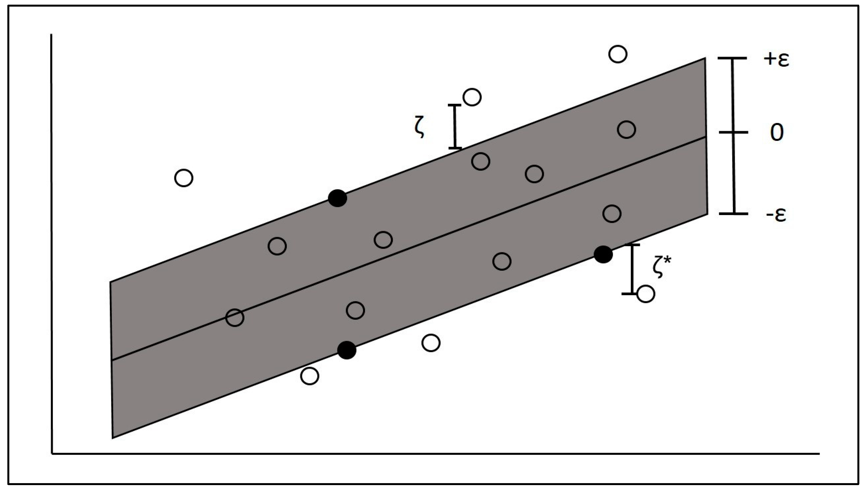
The Support Vector Regression (SVR) stems from the research field of machine learning and it is a direct extension of the Support Vector Machine algorithm. The ability of the SVR in better describing nonlinear and nonstationary phenomena than other econometric techniques has gained the interest of many researchers in economics and finance ( for more details see [24,25,26,27]). The technique was proposed by Cortes and Vapnik in [28] and it attempts to describe actual data observations based on a function where the errors terms do not play any role and are not taken into account as long as they do not violate a predefined threshold ε; only errors higher than ε are penalized. The observations that specify the “error tolerance band” given ε are called Support Vectors (SV) and are located through a minimization procedure.

Unlike other machine learning approaches, the SVR is based on a convex minimization problem with a unique global minimum, avoiding local minima. In order to train the model, we use a large part of the available dataset to pinpoint the SVs, while the remaining observations are utilized to test the generalization ability of the model. A typical approach in avoiding overfit of the model is to use cross-validation training techniques.

For a training dataset $D=\left[\left({\mathit{x}}_1,y_1\right),\left({\mathit{x}}_2,y_2\right),\dots .\left({\mathit{x}}_n,y_n\right)\right],{\mathit{x}}_i\in {\mathbb{R}}^m,y_i\in \mathbb{R},i=1,2,\dots .n,$ where ${\mathit{x}}_i$ is a vector of independent variables and $y_i$ is the dependent variable, the linear regression function takes the form of$y=f\left(\mathit{x}\right)={\mathit{w}}^T\mathit{x}+b$ (where T denotes the transpose). This is achieved by solving:

$$\min \left(\frac{1}{2}\parallel \mathit{w}\parallel {}^2+C{\displaystyle \sum }_{\iota =1}^n\left({\zeta }_i+{\zeta }_i^{*}\right)\right)$$

(1)

$$\mathrm{subject}\mathrm{to}\{\begin{array}{c}{y}_i-\left({\mathit{w}}^T{\mathit{x}}_i+b\right)\le \epsilon +{\zeta }_i\\ \left({\mathit{w}}^T{\mathit{x}}_i+b\right)-y_i\le \epsilon +{\zeta }_i^{*}\\ {\zeta }_i, {\zeta }_i^{*}\ge 0\end{array}$$

where ε defines the width of the tolerance band, and ${\zeta }_i$, ${\zeta }_i^{*}$are slack (penalty) variables controlled through a penalty parameter C (see Figure 1). Points inside the tolerance band are not penalized. System (1) describes a convex quadratic optimization problem with linear constraints, where the first part controls the generalization ability of the regression, through the Euclidean norm $\mathit{w}$. The second part of the objective function controls the fit of the regression to the training data. When the parameter C is increased, we apply a “heavier” penalty on any point outside the error tolerance band i.e., with ${\zeta }_i\ge 0$ or ${\zeta }_i^{*}\ge 0$. The optimum model in the one that finds the balance between the two parts of the objective function.

Using the Lagrange multipliers in System (1), the solution is given by:

$$\mathit{w}={\displaystyle \sum }_{i=1}^n\left(a_i-a_i^{*}\right){\mathit{x}}_i$$

(2)

$$\mathrm{and} y={\sum }_{i=1}^n\left(a_i-a_i^{*}\right){\mathit{x}}_i^T\mathit{x}$$

(3)

with the coefficient ${\alpha }_i$, $a_i^{*}$ = 0 for all non-SVs observations. Nevertheless, most real-life phenomena are nonlinear and they cannot be adequately described using linear models. Given that the SVR is a linear model that finds a linear tolerance band, we extend it by coupling it with kernel functions. The notion of a kernel function is to project the initial dataset into a “richer” dimensional space, where we can find a linear solution, and then return to the initial dimensional space. The so-called “kernel trick” ensures small computational effort, since the projection is achieved using inner products instead of mapping each data point explicitly. The use of a nonlinear kernel function transforms our SVR model into a nonlinear one. In the empirical part of this paper we use the linear and the nonlinear radial basis function (RBF) kernel. The mathematical representation of the two kernels is:

$$\mathrm{Linear} K_1\left({\mathit{x}}_1,{\mathit{x}}_2\right)={\mathit{x}}_1^T{\mathit{x}}_2$$

(4)

$$\mathrm{RBF} K_2\left({\mathit{x}}_1,{\mathit{x}}_2\right)=e^{-\gamma \parallel {\mathit{x}}_1-{\mathit{x}}_2\parallel {}^2}$$

(5)

with γ representing a kernel parameter.

2.2. The Data

To measure geopolitical risk, we compile a dataset of monthly GPR indices for 14 developing countries (Turkey, Mexico, Korea, Russia, India, Brazil, China, Indonesia, Saudi Arabia, Argentina, Thailand, Israel, Malaysia, Philippines) from Caldara and Iacovello as proposed in [19] and we also use data on West Texas Intermediate crude oil prices, gold prices, and exchange rates for the selected national currencies against the U.S. dollar. All variables are from the database of the Federal Reserve Bank of St. Louis (FRED). We also compile stock index prices from Yahoo! Finance for the selected economies, in order to study the relationship between GPR and the financial market. The GPR data spans the period January 1985–May 2018 and it is adjusted according to the availability of the rest of the variables for each country. All of the values are transformed into their logarithmic forms. The descriptive statistics for all variables are reported in

Table 1. Descriptive Statistics.

Countries	Mean	Standard Deviation	Skewness	Kurtosis	Start Date	End Date
Panel A: Exchange rates
Turkey	−1.79	2.95	−0.76	2.00	Dec-84	Apr-18
Mexico	2.37	0.36	−1.19	5.69	Dec-92	Jun-17
Korea	6.89	0.20	−0.17	2.00	Dec-84	May-18
Russia	2.89	1.21	−1.68	5.49	May-92	Mar-18
India	3.58	0.50	−0.96	2.78	Dec-84	May-18
Brazil	0.71	0.38	−0.46	2.52	Dec-94	May-18
China	1.86	0.30	−1.13	3.29	Dec-84	May-18
Indonesia	8.55	0.84	−0.48	1.50	Dec-84	Mar-18
Saudi Arabia	1.32	0.00	−3.69	50.75	Oct-95	May-18
Argentina	1.20	0.87	0.17	2.37	Jul-96	May-18
Thailand	3.46	0.19	0.25	1.78	Dec-84	May-18
Israel	1.15	0.37	−1.32	4.19	Dec-84	Mar-18
Malaysia	1.16	0.18	−0.03	1.53	Dec-84	May-18
Philippines	3.80	0.19	−1.53	5.21	Oct-95	May-18
Panel B: Stock indices
Turkey	8.88	2.61	−0.91	2.44	Dec-89	May-18
Mexico	9.37	1.15	−0.25	1.61	Oct-91	May-18
Korea	6.83	0.66	−0.72	3.50	Dec-84	May-18
Russia	6.56	1.12	−1.10	3.19	Aug-97	May-18
India	8.49	1.29	−0.33	2.12	Dec-84	May-18
Brazil	8.61	3.94	−2.16	6.54	Nov-89	May-18
China	7.35	0.73	−1.27	5.22	Nov-90	May-18
Indonesia	6.69	1.30	−0.11	2.20	Dec-84	May-18
Saudi Arabia	8.37	0.76	−0.30	1.71	Dec-93	May-18
Argentina	6.66	2.39	−2.09	9.16	Dec-87	May-18
Thailand	6.87	0.40	−0.18	1.91	Apr-03	May-18
Israel	6.38	0.69	−0.39	1.73	Aug-92	May-18
Malaysia	7.15	0.33	−0.57	1.97	Jun-02	May-18
Philippines	7.76	0.71	0.14	2.12	Nov-86	May-18
Panel C: Other variables
WTI oil	3.54	0.65	0.36	1.78	Dec-84	May-18
Gold price	6.30	0.60	0.64	1.82	Dec-84	May-18

.

As we observe, all variables are negatively skewed, suggesting that the mass of the distribution is gathered at the left end of the distribution, exhibiting frequent values that are lower than the mean. The kurtosis of the exchange rates is mainly below 3, indicating platykurtic distributions, while for Mexico, Saudi Arabia, Israel, and Philippines, we observe high values that suggest leptokurtic distributions. The same applies for the stock indices of Brazil, China, and Argentina. The leptokurtic distributions imply the existence of extreme values.

3. Empirical Results

In order to study the ability of the GPR index in forecasting a pool of selected variables, we train OLS (We use first differences in all estimations and Newey-West Robust Standard Errors) and SVR regression models in rolling windows. In each step we use 120 observations for training our models. Based on the trained model, we evaluate the forecasting ability in 1, 3, 6, 12, and 24 months ahead forecasting. Afterwards, we slide our training window one observation forward removing the first observation of the previous window as to maintain our training sample at 120 observations and retrain the model. We do so until the end of our sample. After collecting all out-of-sample forecasts, we measure the Mean Absolute Percentage Error (MAPE). All of the models include the first lag of the dependent variable (We also trained models of higher lag order, but the results were quantitatively similar). In the following tables we report the MAPE for the OLS model, the most accurate kernel for the SVR model (All results are available from the authors upon request.) and the MAPE of the Random Walk (RW) model (where we assume that the best forecast is the present value).

3.1. Oil prices

We start our forecasting exercise in evaluating the ability of the GPR index in forecasting oil prices (

Table 2. Oil prices out-of-sample forecasting accuracy—MAPE.

Forecasting Horizons	1 Month			3 Months			6 Months			12 Months			24 Months
Country	OLS	SVR	RW	OLS	SVR	RW	OLS	SVR	RW	OLS	SVR	RW	OLS	SVR	RW
Turkey	6.86	6.86	6.69	15.74	15.63	13.98	28.27	27.34	21.06	42.76	43.64	27.58	50.70	48.98	36.74
Mexico	7.02	7.02	6.68	16.27	16.30	14.68	29.47	28.28	22.65	43.25	42.27	30.05	49.12	47.58	39.64
Korea	6.73	6.68	6.55	15.13	15.49	13.33	25.96	25.79	20.16	36.70	36.32	27.59	44.59	42.95	36.56
Russia	7.21	7.26	6.98	17.77	17.84	16.27	31.68	29.24	25.10	45.89	42.39	32.44	49.35	46.98	43.24
India	6.88	6.77	6.55	15.39	15.12	13.33	25.85	25.15	20.16	35.83	36.56	27.59	42.98	46.78	36.56
Brazil	6.88	6.85	6.77	16.44	16.53	14.97	30.75	29.41	23.05	43.30	44.36	29.97	47.43	51.48	39.16
China	6.82	6.85	6.66	15.55	15.78	14.23	27.95	26.48	21.53	39.65	40.02	28.45	51.47	55.24	37.54
Indonesia	6.71	6.82	6.57	15.31	15.66	13.41	26.23	25.80	20.24	35.51	36.63	27.79	41.83	45.70	36.64
Saudi Arabia	6.89	6.98	6.71	17.37	16.96	15.25	33.22	30.54	23.70	48.40	48.72	30.54	47.01	49.21	40.81
Argentina	6.91	7.02	6.82	17.75	17.81	15.70	34.02	32.23	24.51	47.70	46.60	32.15	49.75	52.64	41.60
Thailand	7.02	7.15	6.56	18.83	18.41	14.64	37.63	35.45	21.86	62.67	66.68	35.20	85.87	89.41	77.78
Israel	6.87	6.83	6.73	15.73	15.63	14.43	29.08	27.73	21.73	43.46	43.92	28.90	51.54	55.64	39.69
Malaysia	6.44	6.53	6.46	14.61	15.15	13.95	27.38	25.30	19.71	54.06	53.62	31.25	78.61	78.91	64.72
Philippines	6.84	6.84	6.71	16.25	16.58	15.25	31.92	30.11	23.70	45.95	45.07	30.54	50.95	56.62	40.81

Note: All values are percentages. Although the oil prices (dependent variable) used for all countries are the same, the different MAPE of the RW model is attributed to the different number of out-of-sample forecasts for each country, according to the availability of the data so that the comparison between the dependent variables could be feasible.

). Given that the dependent variable for all models is the WTI oil prices, we consider the country specific GPR index of each economy and the first lag of the WTI dependent variable as regressors. As we observe, the OLS and the SVR models exhibit similar forecasting performance and they both fail to outperform the RW model. Their performance is worse in the longer than the shorter horizons in MAPE terms. In these cases, the markets appear efficient, since we cannot outperform the RW model. Thus, trying to forecast these time series is impossible and any comparison between the two forecasting models is redundant. Thus, the GPR index has limited ability in foreseeing future oil price fluctuations, since it fails to outperform a simple guess about the future value of oil prices. This finding is interesting, especially for oil exporting countries such as Saudi Arabia, where we would expect that conflicts and terrorist acts that affect oil inventories would influence oil prices. Thus, unlike [19], who argue that their GPR index adheres to oil price fluctuations closely, our out-of-sample forecasting exercise reveals that the “true” forecasting ability of the emerging economies’ index is limited, regardless of the economy under examination, oil producing or not. This finding could be attributed to the way that the index is constructed, since most articles in leading global newspapers have limited coverage of peripheral incidents and especially for emerging economies.

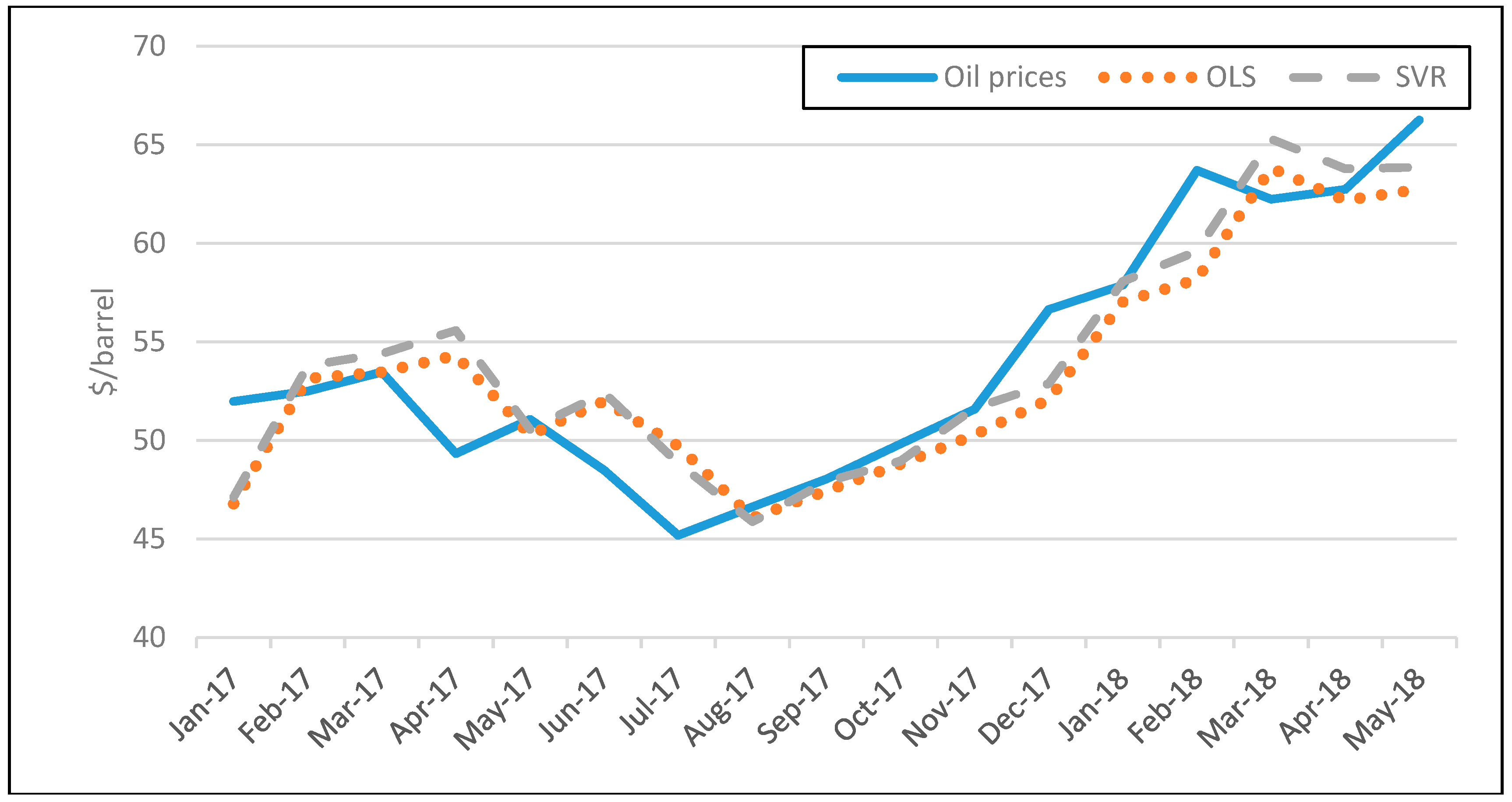
To visualise the forecasts of our models, in Figure 2 we depict the actual and the forecasted oil prices for Saudi Arabia in the one-month ahead and in Figure 3 in the 12-months ahead forecasting windows respectively, for the period Jan-2017 to May-2018. The selection of the Saudi Arabia over the other emerging economies is motivated by the fact that oil is the main exporting commodity of this economy. We graph only the 17 last forecasts so that the figures are readable.

As expected, in the shorter one-month horizon, both models adhere closely to the actual oil prices, while in the longer 12-month forecasts they fail to capture the “true” data generating mechanism. This fact could be justified by the larger uncertainty in forecasting oil prices in longer horizons, given that the macroeconomic conditions and especially the demand for oil that significantly affects its price is volatile in longer forecasting horizons.

3.2. Exchange Rates

Next, we evaluate the ability of the GPR index in forecasting exchange rates. The dependent variable in each model for each country is the exchange rate of the national currency against the U.S. dollar, while the independent variables are the lagged exchange rate and the country specific GPR index of the developing economy under examination. The forecasting accuracies in terms of the MAPE are reported in

Table 3. Exchange rate out-of-sample forecasting accuracy—MAPE.

Forecasting Horizons	1 Month			3 Months			6 Months			12 Months			24 Months
Country	OLS	SVR	RW	OLS	SVR	RW	OLS	SVR	RW	OLS	SVR	RW	OLS	SVR	RW
Turkey	2.97	2.90	2.82	6.67	6.30	5.92	11.05	10.56	8.97	19.04	18.61	13.73	40.65	32.29	18.72
Mexico	1.82	1.84	1.83	3.78	3.88	3.84	5.59	5.68	5.33	8.74	9.41	7.97	13.06	14.68	11.41
Korea	1.96	1.93	1.80	4.98	4.22	3.72	8.25	6.44	5.78	13.87	10.72	9.17	15.04	12.75	13.77
Russia	3.23	3.25	3.15	7.29	7.09	6.61	9.19	9.83	8.96	17.12	16.86	13.04	25.84	23.08	19.85
India	1.16	1.14	1.08	2.53	2.51	2.35	4.05	4.17	3.64	6.92	7.42	6.19	9.71	10.64	9.35
Brazil	2.99	3.11	2.69	6.87	6.54	5.66	12.26	11.09	9.22	19.61	17.86	14.33	32.38	31.82	19.57
China	0.38	0.36	0.34	0.94	0.93	0.88	1.76	1.74	1.56	3.65	4.08	2.78	10.61	11.72	5.07
Indonesia	3.68	3.39	3.21	7.60	6.73	6.13	14.53	9.63	8.53	30.34	14.93	12.70	61.78	22.22	18.19
Saudi Arabia	0.05	0.05	0.06	0.05	0.05	0.06	0.05	0.05	0.07	0.05	0.05	0.07	0.05	0.05	0.07
Argentina	1.85	1.68	1.82	5.12	4.28	4.63	9.76	7.25	7.85	17.16	16.32	14.26	22.20	24.52	27.12
Thailand	1.02	1.01	1.01	2.22	2.10	2.12	3.79	3.85	3.39	5.94	6.32	5.23	7.62	7.84	8.66
Israel	1.78	1.81	1.72	3.39	3.47	3.15	5.23	5.38	4.73	7.15	7.39	6.72	10.75	9.91	8.06
Malaysia	1.65	1.63	1.59	3.67	3.63	3.41	6.19	6.42	4.68	10.11	10.83	7.85	19.01	19.00	13.57
Philippines	1.18	1.15	1.12	2.68	2.78	2.42	4.57	4.69	5.94	7.53	7.89	5.87	11.40	12.09	8.21

Note: All values are percentages.

. As with the oil prices, no model consistently outperforms the RW model, except for Saudi Arabia in all forecasting horizons and Philippines in the three and six-month ahead forecasting window, where both the OLS and the SVR model outperform the RW. In the case of Saudi Arabia, the OLS and the SVR model exhibit similar performance, while in the Philippine peso, the OLS model has lower forecasting error than the SVR one. Nevertheless, the forecasting performance in the case of the Philippine peso is episodical, since it disappears in all other forecasting horizons.

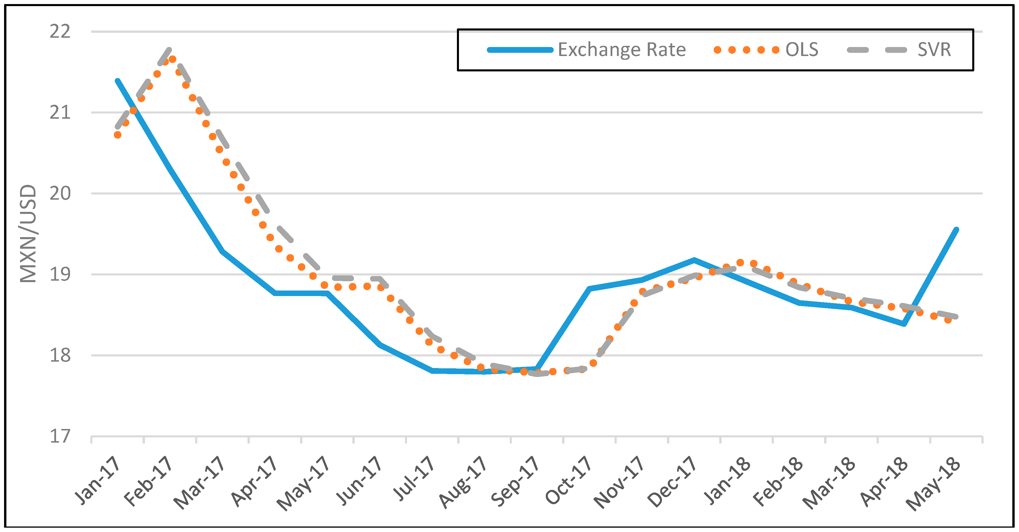
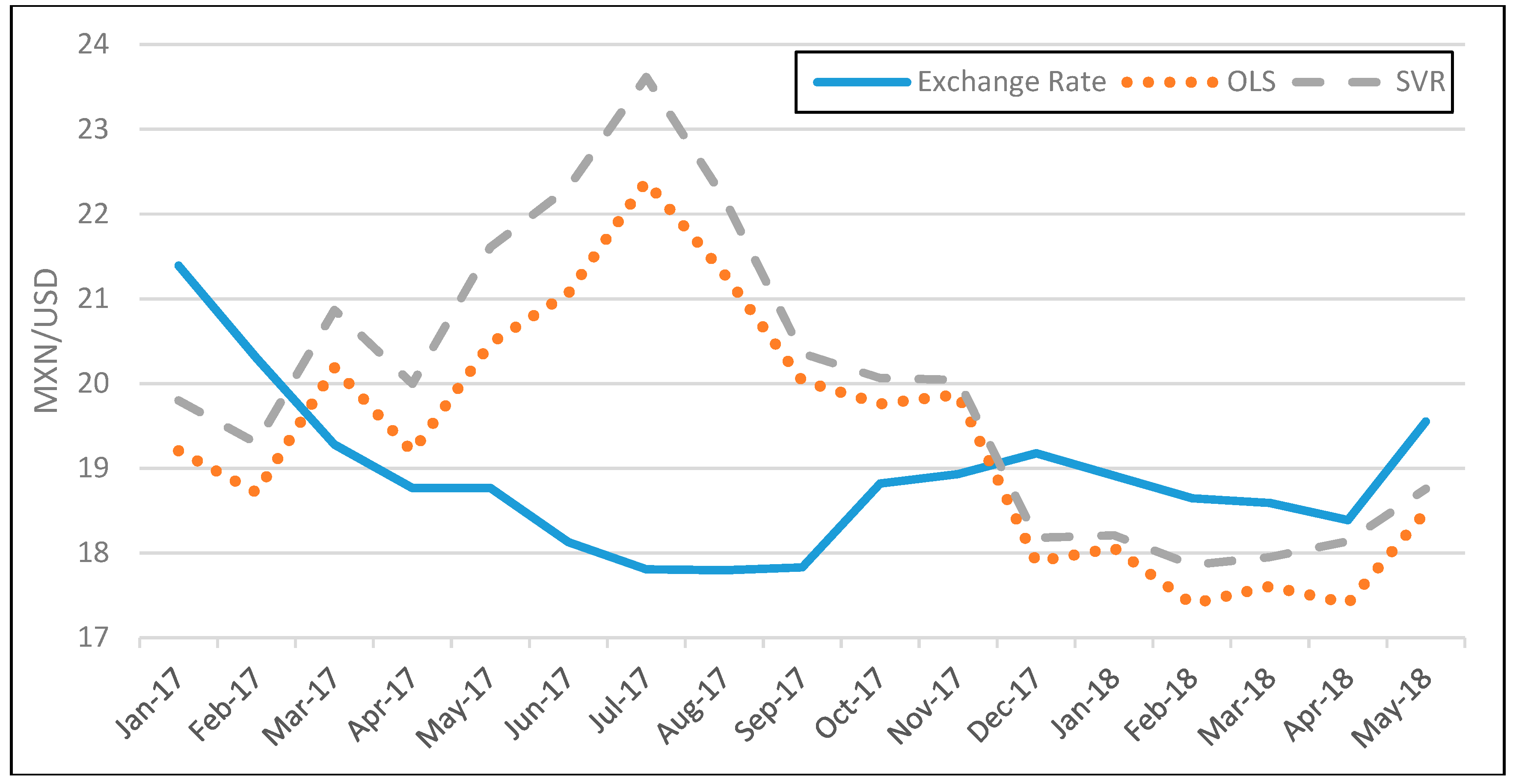
Our findings suggest that the GPR index of the emerging countries has a limited predictive power on exchange rates. As we discuss in the introductory section, the effect of a terrorist attack or a conflict on the exchange rates is transitory and probably not obvious on our monthly dataset. As an example, in Figure 4 and Figure 5, we depict the actual and the forecasted exchange rates for Mexico in one-month and 12-months ahead forecasting windows, respectively.

As we observe, both models produce similar forecasts, which are consistently diverging from the actual exchange rate values, especially in the longest 12-month forecasting horizon. The fact that the GPR indices of emerging countries do not adhere to the data generating process of exchange rates might be attributed to the small potential impact of peripheral geopolitical tensions to the exchange rate markets, as stated in [7].

3.3. Stock Indices

In

Table 4. Stock Indices out-of-sample forecasting accuracy—MAPE.

Forecasting Horizons	1 Month			3 Months			6 Months			12 Months			24 Months
Country	OLS	SVR	RW	OLS	SVR	RW	OLS	SVR	RW	OLS	SVR	RW	OLS	SVR	RW
Turkey	7.84	7.70	7.63	13.33	12.85	12.10	22.26	21.80	17.35	35.86	35.07	24.18	66.99	47.70	27.88
Mexico	3.64	3.62	3.68	6.90	7.09	6.63	11.31	11.69	10.16	21.18	22.32	15.76	40.06	39.75	21.64
Korea	5.55	5.54	5.47	10.53	10.52	10.25	16.25	16.55	14.85	24.19	24.72	22.12	26.46	26.28	26.23
Russia	5.62	5.54	5.30	12.04	11.60	10.63	20.33	19.55	17.09	33.08	32.08	23.65	40.08	19.85	19.90
India	5.41	5.48	5.39	9.86	10.04	9.58	15.30	15.41	13.87	24.83	24.22	20.36	35.30	35.86	25.75
Brazil	5.20	5.21	5.09	10.00	10.05	9.63	15.57	16.03	14.40	22.03	23.28	19.68	32.90	31.02	21.09
China	5.83	6.00	5.80	11.95	12.02	11.44	19.25	18.44	17.76	24.57	23.50	25.73	41.07	33.80	30.19
Indonesia	5.54	5.56	5.52	11.15	11.24	10.83	17.05	17.22	16.22	27.46	29.24	23.62	33.54	34.33	28.08
Saudi Arabia	6.00	6.45	5.83	11.54	12.50	11.18	20.02	21.40	16.98	38.68	40.42	26.67	75.58	70.66	30.84
Argentina	7.63	7.49	7.39	13.86	13.86	13.81	21.97	22.00	21.68	37.13	36.42	34.51	46.62	50.09	42.79
Thailand	2.80	2.83	2.72	5.54	5.83	5.08	8.41	8.50	7.61	10.50	10.80	11.10	12.47	18.90	7.69
Israel	3.74	3.75	3.71	7.41	7.78	7.18	12.45	12.58	11.04	21.73	21.71	16.98	29.11	30.16	21.04
Malaysia	1.77	1.75	1.76	2.93	2.96	2.85	4.02	3.96	3.72	8.18	7.00	6.30	7.93	9.06	8.64
Philippines	4.22	4.13	4.13	8.57	8.46	8.02	14.76	14.60	13.02	23.26	22.83	19.49	27.43	31.67	25.17

Note: All values are percentages.

, we report the forecasting performance of our forecasting models in forecasting the national stock index of each developing economy, using the GPR index and the lagged value of the stock index as regressors. This empirical setting of employing machine learning and the specific GPR index in forecasting the stock markets of developing economies has not been used before in the relevant literature.

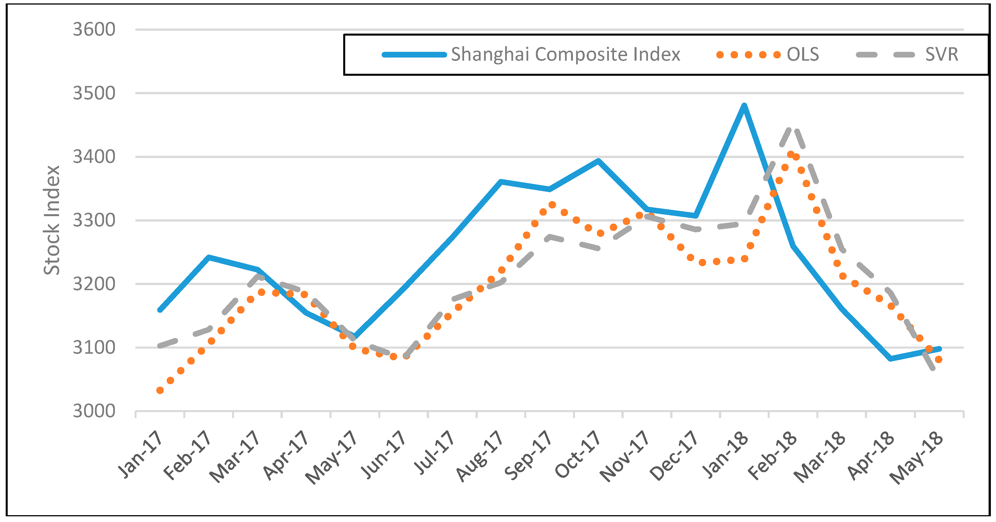
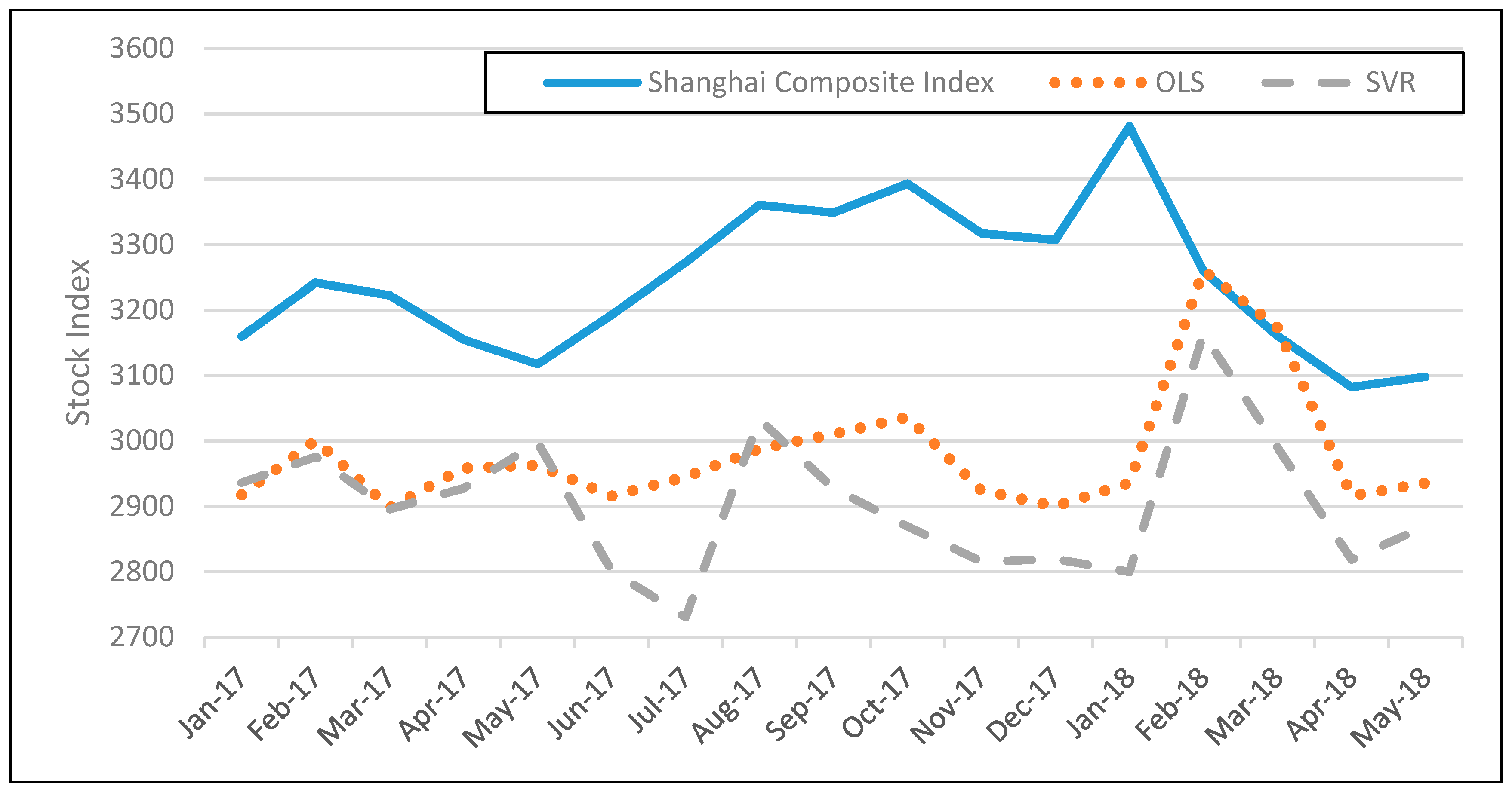
In all countries and horizons, neither the OLS nor the SVR outperform the RW model, except for the SVR model for Mexico, Argentina, and Malaysia in the one-month forecasting horizon. The efficacy of the GPR index in forecasting the national stock index is rather limited, given the transitory nature of geopolitical shocks on stock prices that cannot be detected in our monthly dataset. In Figure 6 and Figure 7, we depict the actual and the forecasted values of the Shanghai Composite index for the one-month and the 12-months ahead forecasting, which represents the index with the largest capitalization among the emerging economies in our sample. As expected, the deviations of the models’ forecasts that form the actual data are larger on the yearly than the monthly forecasting horizon.

3.4. Gold Prices

Finally, we evaluate the ability of the GPR index in forecasting gold prices. Although gold is a commodity, its use as a “safe-heaven” investment during periods of economic and political turmoil renders the examination of gold prices based on geopolitical risk parameters very interesting. Τhe dependent variable in all models is the price of gold, with explanatory variables being the lagged price of gold, and the respective GPR index of the developing country under examination. In

Table 5. Gold prices out-of-sample forecasting accuracy—MAPE.

Forecasting Horizons	1 Month			3 Months			6 Months			12 Months			24 Months
Country	OLS	SVR	RW	OLS	SVR	RW	OLS	SVR	RW	OLS	SVR	RW	OLS	SVR	RW
Turkey	3.83	3.90	7.63	6.11	6.16	12.10	8.70	8.71	17.35	15.33	15.65	24.18	31.74	32.55	27.88
Mexico	4.20	4.20	3.68	6.75	6.85	6.63	9.51	9.51	10.16	16.08	16.32	15.76	35.24	36.08	21.64
Korea	3.56	3.58	5.47	6.04	5.93	10.25	8.55	8.58	14.85	14.58	15.06	22.12	30.78	31.50	26.23
Russia	4.16	4.27	5.30	6.79	6.83	10.63	8.80	9.22	17.09	15.25	15.59	23.65	33.40	34.53	19.90
India	3.56	3.55	5.39	5.99	5.95	9.58	8.47	8.53	13.87	14.31	14.88	20.36	31.15	32.50	25.75
Brazil	4.06	4.08	5.09	6.68	6.70	9.63	9.31	9.42	14.40	15.75	16.21	19.68	32.67	33.65	21.09
China	3.86	3.89	5.80	6.49	6.51	11.44	8.94	9.03	17.76	15.28	15.90	25.73	31.44	32.98	30.19
Indonesia	3.60	3.61	5.52	5.95	5.83	10.83	8.51	8.42	16.22	14.46	14.89	23.62	31.41	32.76	28.08
Saudi Arabia	4.07	4.14	5.83	6.74	6.75	11.18	9.05	9.10	16.98	14.20	14.77	26.67	30.31	31.96	30.84
Argentina	4.01	4.05	7.39	6.61	6.65	13.81	8.72	8.82	21.68	14.51	14.97	34.51	30.51	31.61	42.79
Thailand	3.45	3.39	2.72	5.72	5.74	5.08	6.80	6.74	7.61	9.69	9.70	11.10	19.25	20.99	7.69
Israel	4.05	4.03	3.71	6.44	6.55	7.18	8.97	8.90	11.04	14.87	15.05	16.98	31.46	32.81	21.04
Malaysia	3.36	3.35	1.76	5.95	6.51	2.85	8.47	8.65	3.72	15.58	15.90	6.30	33.97	35.89	8.64
Philippines	4.11	4.15	4.13	6.78	6.78	8.02	9.20	9.07	13.02	14.74	15.53	19.49	30.86	32.11	25.17

Note: All values are percentages. Although the gold prices used for all countries are the same, the different MAPE of the RW model is attributed to the different number of out-of-sample forecasts for each country, according to the availability of the data so that the comparison between the dependent variables could be feasible.

, we report the forecasting performance of our forecasting models in forecasting the gold prices, using the GPR index and the lagged value of gold prices as regressors.

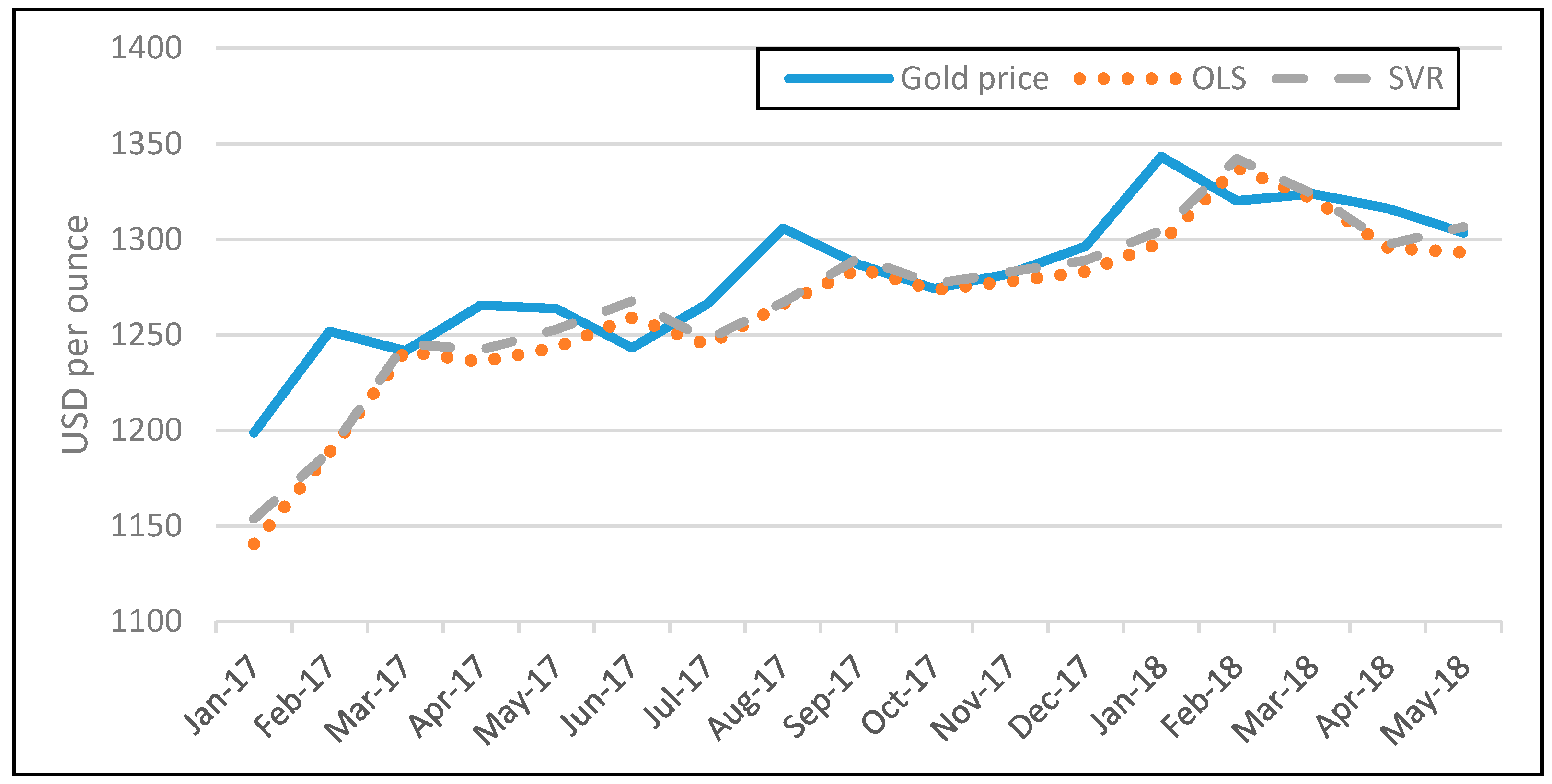
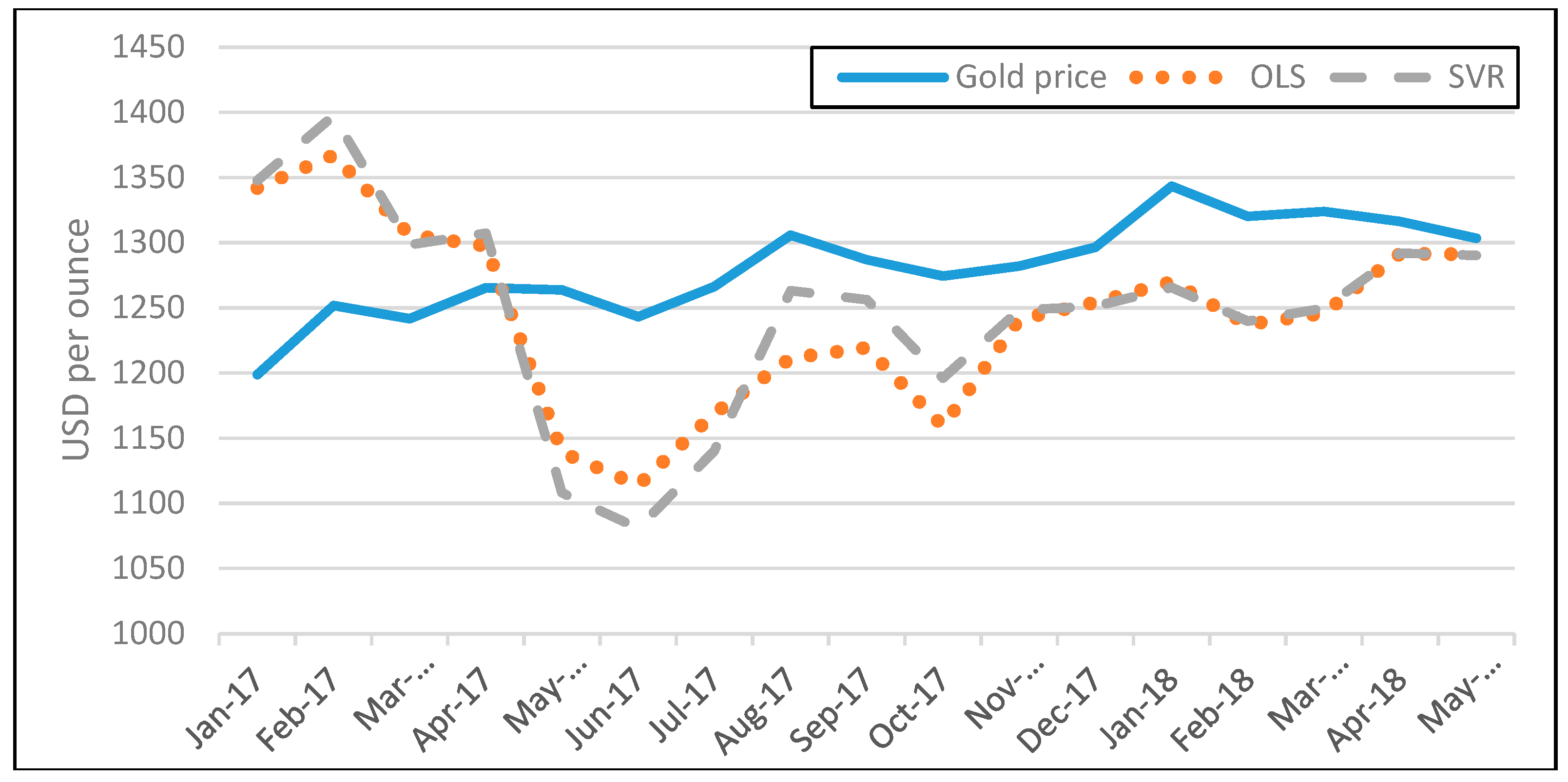
As we observe, both models outperform the RW model for most countries and in most forecasting horizons up to 12 months. More specifically, in the one-month forecasting horizon, both models outperform the RW model in the case of Turkey, Korea, Russia, India, Brazil, China, Indonesia, Saudi Arabia, and Argentina. In eight out of these nine countries, the OLS model is more accurate than the SVR. In the three-month forecasting horizon, the list of the nine countries is expanded to 11 countries, adding Israel and Philippines. In nine out of these 11 countries, the OLS model is more accurate that the SVR one. In the six-month forecasting horizon, all models—except those for Malaysia—outperform the RW model, where again in nine out of the 13 countries, the OLS model is the most accurate, while in the 12-month horizon we revert to the initial list of countries of the one-month forecasting horizon. In the longer 24-month forecasting horizon, the ability of all models to outperform the RW model is completely lost. This finding suggests that the GPR indices can forecast gold prices with consistency based on the GPR index of most countries for up to 12 months ahead, while we do not find evidence in favor of using the SVR over the OLS model for one-month up to 12-months ahead forecasting. In Figure 8 and Figure 9, we depict the gold price forecasts on one- and 12-months ahead for China. The selection of China is motivated by the fact that China is the largest gold producing country in the world, with 440 tons in 2017 as documented in [29].

Apparently, in the shorter horizon, both models adhere more closely to gold prices than in the longest 12-month horizon. The ability of the GPR indices of emerging economies to forecast gold price fluctuations more accurately than the RW model is detected in the case of Turkey, Korea, Russia, India, Brazil, China, Indonesia, Saudi Arabia, and Argentina consistently up to 12-months ahead forecasting, suggesting the direct link between gold prices and risk management investing decisions.

4. Conclusions

In this paper, we attempt to forecast a list of variables, namely the price of oil, national exchange rates, national stock market indices, and the price of gold for fourteen developing economies. In doing so, we employ the Geopolitical Risk index of Caldara and Iacovello, as a leading indicator. The analysis is performed using data from the period January 1985–May 2018, which is adjusted according to the availability of the rest of the variables for each country. We train machine learning models based on the Support Vector Regression technique and measure their forecasting ability in several forecasting horizons, namely, 1-, 3-, 6-, 9-, 12-, and 24-months ahead. We also compare the results with a traditional OLS model, and moreover, the naïve Random Walk model is used as a benchmark reference model to compare the performance of the two others. Thus, our empirical findings suggest that the geopolitical risk (the GPR index) in emerging countries has no forecasting ability over the three of the four variables under examination, since it fails to provide models that outperform the simple RW model. In contrast, we find that the GPR index appears to possess significant forecasting ability on gold prices, as is captured by our models.

These empirical findings may provide some relevant policy implications. As the effects of geopolitical tensions on oil prices, exchange rates and stock prices, appear to be temporary, both governments and economic agents must be cautious and not overreact to the initial price fluctuations in the aftermath of geopolitical tensions. The exception is the case of gold, where these tensions appear to have a significant lasting effect, confirming that gold is used as a safe haven by investors.

Overall, we do not find empirical evidence on a link between oil prices, exchange rates, stock indices, and geopolitical tensions in emerging economies. This finding could be attributed to the peripheral character of political conflicts in emerging economies that fail to spillover into the global market. As expected, gold prices seem to be driven by political risk, given that throughout history gold is used as a safe haven to hedge uncertainty and risk [30].

References

- Carney, M. Uncertainty, the Economy and Policy; Bank of England: London, UK, 2016. [Google Scholar]
- European Central Bank. Economic Bulletin, Frankfurt, 2017, 3. Available online: https://www.ecb.europa.eu/pub/economic-bulletin/html/eb201703.en.html (accessed on 20 December 2018).
- International Monetary Fund. Seeking Sustainable Growth: Short-Term Recovery, Long-Term Challenges. Washington, DC, USA, October 2017. Available online: https://www.imf.org/~/media/Files/Publications/WEO/2017/October/pdf/main-chapter/text.ashx (accessed on 20 December 2018).
- Alesina, A.; Ozler, S.; Roubini, N.; Swagel, P. Political instability and economic growth. J. Econ. Growth 1996, 1, 189–211. [Google Scholar] [CrossRef] [Green Version]
- Asteriou, D.; Siriopoulos, C. The role of political instability in stock market development and economic growth: The case of Greece. Econ. Notes 2000, 29, 355–374. [Google Scholar] [CrossRef]
- Kollias, C.; Papadamou, S.; Siriopoulos, C. Terrorism Induced Cross-Market Transmission of Shocks: A Case Study Using Intraday Data; Economics of Security Working Paper, No. 66; Deutsches Institut für Wirtschaftsforschung (DIW): Berlin, Germany, 2012. [Google Scholar]
- Blomberg, B.; Hess, G.; Jackson, H. Terrorism and the returns to oil. Econ. Politics 2009, 21, 409–432. [Google Scholar] [CrossRef]
- Antonakakis, N.; Gupta, R.; Kollias, C.; Papadamou, S. Geopolitical risks and the oil-stock nexus over 1899–2016. Financ. Res. Lett. 2017, 23, 165–173. [Google Scholar] [CrossRef]
- Kollias, C.; Kyrtsou, C.; Papadamou, S. The Effects of Terrorism and War on the Oil Price–stock Index Relationship. Energy Econ. 2013, 40, 743–752. [Google Scholar] [CrossRef]
- Drakos, K. Terrorism activity, investor sentiment and stock returns. Rev. Financ. Econ. 2010, 19, 128–135. [Google Scholar] [CrossRef]
- Kollias, C.; Papadamou, S.; Stagiannis, A. Stock markets and terrorist attacks: Comparative evidence from a large and a small capitalization market. Eur. J. Political Econ. 2011, 27 (Suppl. 1), S64–S77. [Google Scholar] [CrossRef]
- Nikkinen, J.; Omran, M.; Sahlstrom, P.; Aijo, J. Stock returns and volatility following the September 11 attacks: Evidence from 53 equity markets. Int. Rev. Financ. Anal. 2008, 17, 27–46. [Google Scholar] [CrossRef]
- Gupta, R.; Majumdar, A.; Pierdzioch, C.; Wohar, M.E. Do Terror Attacks Predict Gold Returns? Evidence from a Quantile-Predictive-Regression Approach. Q. Rev. Econ. Financ. 2017, 65, 276–284. [Google Scholar] [CrossRef]
- International Monetary Fund. How has September 11 influenced the global economy. In World Economic Outlook; International Monetary Fund: Washington, DC, USA, 2001; Chapter 2; pp. 14–33. [Google Scholar]
- Balcilar, M.; Gupta, R.; Pierdzioch, C.; Wohar, M. Do terror attacks affect the dollar-pound exchange rate? A nonparametric causality-in-quantiles analysis. N. Am. J. Econ. Financ. 2017, 41, 44–56. [Google Scholar] [CrossRef]
- Filippou, I.; Gozluklu, A.; Taylor, M. Global Political Risk and Currency Momentum. J. Financ. Quant. Anal. 2018, 53, 2227–2259. [Google Scholar] [CrossRef]
- Suleman, M.T. Political Uncertainty, Exchange Rate Return and Volatility. 2015. Available online: https://ssrn.com/abstract=2598866 (accessed on 1 October 2018).
- Cosset, J.C.; Doutriaux De La Rianderie, B. Political Risk and Foreign Exchange Rates: An Efficient-Market Approach. Int. J. Bus. Stud. 1985, 16, 21–55. [Google Scholar] [CrossRef]
- Caldara, D.; Iacovello, M. Measuring Geopolitical Risk. Board of Governors of the Federal Reserve System; International Finance Discussion Paper; Federal Reserve: Washington, DC, USA, 2018; No. 1222. [Google Scholar]
- Davis, S. Policy Uncertainty vs. the VIX: Streets and Horizons. In Proceedings of the Federal Reserve Board Workshop on Global Risk, Uncertainty, and Volatility, Washington, DC, USA, 25 September 2017. [Google Scholar]
- Mensi, W.; Beljid, M.; Boubaker, A.; Managi, S. Correlations and Volatility Spillovers across Commodity and Stock Markets: Linking Energies, Food, and Gold. Econ. Model. 2013, 32, 15–22. [Google Scholar] [CrossRef]
- Mullainathan, S.; Spiess, J. Machine Learning: An Applied Econometric Approach. J. Econ. Perspect. 2017, 31, 87–106. [Google Scholar] [CrossRef] [Green Version]
- Campbell, J.Y. Viewpoint: Estimating the equity premium. Can. J. Econ. 2008, 41, 1–21. [Google Scholar] [CrossRef]
- Khandani, A.E.; Kim, A.J.; Lo, A.W. Consumer credit-risk models via machine-learning algorithms. J. Bank. Financ. 2010, 34, 2767–2787. [Google Scholar] [CrossRef] [Green Version]
- Öğüt, H.; Doğanay, M.M.; Ceylan, N.B.; Aktaş, R. Prediction of bank financial strength ratings: The case of Turkey. Econ. Model. 2012, 29, 632–640. [Google Scholar] [CrossRef]
- Plakandaras, V.; Gupta, R.; Gogas, P.; Papadimitriou, T. Forecasting the U.S., Real House Price Index. Econ. Model. 2015, 45, 259–267. [Google Scholar] [CrossRef]
- Rubio, G.; Pomares, H.; Rojas, I.; Herrera, L.J. A heuristic method for parameter selection in LS-SVM: Application to time series prediction. Int. J. Forecast. 2011, 27, 725–739. [Google Scholar] [CrossRef]
- Cortes, C.; Vapnik, V. Support-Vector Networks. Mach. Learn. 1995, 20, 273–297. [Google Scholar] [CrossRef]
- U.S. Geological Survey. Mineral Commodity Summaries 2018; U.S. Geological Survey: Reston, VA, USA, 2018.
- Jones, A.; Sackley, W. An uncertain suggestion for gold-pricing models: The effect of economic policy uncertainty on gold prices. J. Econ. Financ. 2106, 40, 367–379. [Google Scholar] [CrossRef]
Figure 1.
The Support Vectors (black filled circles) define the boundaries of the error tolerance band. Forecasted values greater than get a penalty equal to ζ according to their deviation from the tolerance band.
Figure 2.
Out-of-sample 1-month ahead oil prices forecasts based on the Saudi Arabia geopolitical risk (GPR) index for the Support Vector Regression (SVR) and Ordinary Least Square (OLS) model for the period Jan-2017 to May-2018.
Figure 3.
Out-of-sample 12-month ahead oil prices forecasts based on the Saudi Arabia GPR index for the SVR and OLS model for the period Jan-2017 to May-2018.
Figure 4.
Out-of-sample 1-month ahead exchange rate forecasts for Mexico based on the GPR index for the SVR and OLS model for the period Jan-2017 to May-2018.
Figure 5.
Out-of-sample 12-month ahead exchange rate forecasts for Mexico based on the GPR index for the SVR and OLS model for the period Jan-2017 to May-2018.
Figure 6.
Out-of-sample 1-month ahead exchange rate forecasts for the Shanghai Composite index based on the GPR index for the SVR and OLS model for the period Jan-2017 to May-2018.
Figure 7.
Out-of-sample 12-month ahead exchange rate forecasts for the Shanghai Composite index based on the GPR index for the SVR and OLS model for the period Jan-2017 to May-2018.
Figure 8.
Out-of-sample one-month ahead gold prices forecasts for China based on the GPR index for the SVR and OLS model for the period Jan-2017 to May-2018.
Figure 9.
Out-of-sample 12-month ahead gold prices forecasts for China based on the GPR index for the SVR and OLS model for the period Jan-2017 to May-2018.