Abstract
This paper develops the mathematical modeling and deflection control of a textile-reinforced composite integrated with shape memory actuators. The mathematical model of the system is derived using the identification method and an unstructured uncertainty approach. Based on this model and a robust stability analysis, a robust proportional–integral controller is designed for controlling the deflection of the composite. We showed that the robust controller depends significantly on the modeling of the uncertainty. The performance of the proposed controller is compared with a classical one through experimental analysis. Experimental results show that the proposed controller has a better performance as it reduces the overshoot and provide robustness to uncertainty. Due to the robust design, the controller also has a wide operating range, which is advantageous for practical applications.
1. Introduction
Soft robots have been used in a wide range of applications. Considerable growth in the application area is expected in the coming years [1,2]. The growing interest in soft robots comes from the good performance of these materials in environments which is not best suited for conventional rigid bodies. Soft robots utilize the compliance, adaptability, and flexibility of soft materials and actuation methods to develop highly adaptive structures [3]. Soft robots are mainly composed of materials with low Young’s modulus (around 1 GPa). Typical materials to which this applies are silicone, rubber, or other elastomeric polymers. The strength and stiffness of these soft materials can be improved by adding reinforcement materials such as fibers. The resulting combination called textile reinforced composites is lightweight, strong, and resistant that makes it ideal for diverse soft robotics applications [4,5]. Engineering applications of these composites exist in robotics, aerospace, automotive, underwater vehicles, and other areas [6].
The elastic properties of textile reinforced composites require smart actuators which possess adaptability and deformability. Smart materials which include piezoelectric materials, shape memory alloys (SMA), and dielectric elastomers have been used in diverse flexible structures [7,8,9]. Among these smart materials, SMAs have the advantages of simple structure, small size, excellent (i.e., higher) force to weight ratio, large displacement, and high stiffness [10,11]. SMAs are capable of returning to a predefined shape when heated. This phenomenon is called the shape memory effect (SME) and is due to crystalline phase transformation from martensite (low temperature phase) to austenite (high temperature phase) [12]. This transformation gives rise to a hysteresis effect which is highly nonlinear. While contracted upon heating, the SMAs exerts a force which is used for actuation. One of the efficient methods for heating the SMAs is resistive heating from an electrical current. Through this method, the deflection and retraction of the wire can be made controllable.
The performance of a shape memory actuator depends significantly on the accuracy of its controls, which is in turn dependent on the SMAs mathematical model. Among the different modeling approaches available in the literature, phenomenological or macro approaches are more suitable to be used for engineering applications. This includes constitutive models like the Tanaka model [13], the Liang and Rogers model [14], the Brinson model [15], and the hysteresis models such as the Preisach model [16], the Krasnosel’skii–Pokrovskii model [17], and the Prandtl–Ishlinskii model [18]. However, due to the complicated dynamics of the hysteresis effect in SMAs, these models are mainly complex and difficult to use for designing a suitable controller. Furthermore, not only the modeling of the involved SMA actuators is required, but of the structure of the entire system as well. One alternative for obtaining the mathematical model of the system is using experimental modeling or system identification to derive simpler equations [19,20]. The nonlinear relationship between the inputs and outputs of the system can be then represented by a linear transfer function which includes the nonlinearities of the system as unstructured uncertainty.
The purpose of this paper is to use the unstructured uncertainty approach for modeling a textile-reinforced composite system actuated by shape memory alloys. The paper extends preliminary findings presented in the conference paper [21]. Different uncertainty models are introduced, applied to the system and consequently compared. Based on the robust stability analysis a proportional–integral controller is then designed to verify the effectiveness of this approach. The objective of the controller is to stabilize the position of the system for a fixed reference. The performance of this controller is compared with a classical one.
The rest of the paper is organized as follows. In Section 2 we describe the test bench. The system identification is addressed in Section 3. We carry out classical controller design in Section 4. The main contribution is the design of a robust controller discussed in Section 5. Finally, we will draw some conclusions in Section 6.
2. System Description
Figure 1 shows the experimental platform of the textile-reinforced composite with integrated SMA actuators. It consists of a textile composite manufactured from a fabric for reinforcement, covered with silicone rubber matrix. For the SMA, we used wires of a Ni-Ti alloy with a protective glass fiber polypropylene sheathing. The sheathed SMA wires are integrated in a strengthening textile in the form of a single-layer plain glass fiber fabric. This fabric was embedded in a castable two-component silicone rubber matrix forming a composite panel. Details of the specimen production as well as the properties of the materials are described in [22]. For our experiments one single specimen was available, but it was tested under different operating conditions.
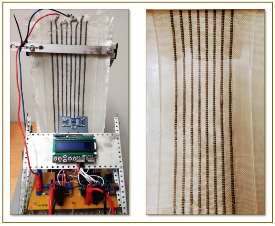
Figure 1.
Test bench of textile-reinforced composite specimen with integrated shape memory alloys (SMAs).
In the composite, the SMAs are placed close to the top surface so that there is a large offset to the center of the material. By this arrangement a phase transition of the SMA wires will bend the composite as shown in Figure 2. When thermally activated through heating, the SMA actuators contract themselves and generate a mechanical tension inside the textile composite. The SMA thermal stimulus is induced by applying a voltage causing a current flow through the wires.
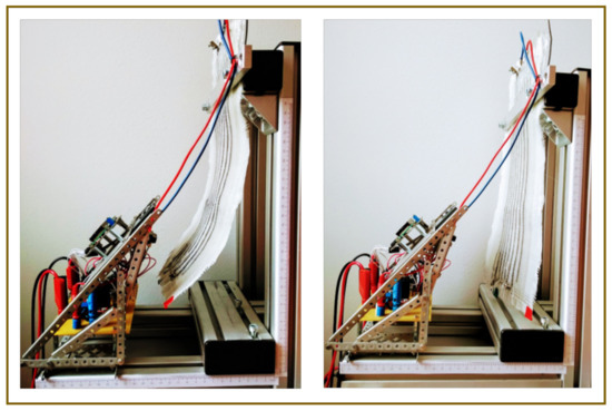
Figure 2.
Deflection of the textile-reinforced composite with side view of the test bench unit.
The voltage to heat the SMAs is provided by a 30 V DC power supply and controlled by an L298N driver IC [23] via pulse width modulation (PWM) with a maximum permissible current of 2 A. This corresponds to a maximum power consumption of 60 W. To measure the deflection of the textile composite we equipped the test bench with a distance sensor of the type GP2Y0A41SK0F from Sharp [24,25]. The control algorithms have been implemented on an Arduino Uno R3 board [25] using the Simulink Support Package for Arduino Hardware [26]. More details on the experimental setup are presented in [21,22].
3. Model Identification
One of the main shortcomings of the SMA actuators is the difficulties in motion control due to hysteresis and other nonlinearities. The reason that gives rise to hysteresis is that the material’s crystalline structure shifts between martensite and austenite phases depending on the applied temperature and stress. Martensite is the rather soft and easily deformed phase of shape memory alloys. This phase exists at lower temperatures, whereas at higher temperatures, the austenite phase is relatively hard. The hysteresis of the shape memory actuators of the experimental platform for four consecutive heating up and cooling down cycles is shown in Figure 3.
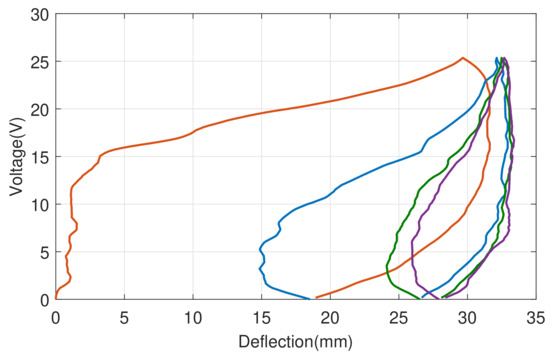
Figure 3.
Four consecutive heating up and cooling down cycles of shape memory alloy with hysteresis.
The system responds with a time lag to the applied voltage. In addition, there is almost no overshoot. For these reasons, we want to describe the system’s essential behavior by a first order linear time-invariant system. In the Laplace frequency domain, the system is modeled by the transfer function
with the complex variable s representing the excitation frequency. In addition, the parameter describes the gain and the parameter is the system’s time constant. Roughly speaking, the transfer function in Equation (1) can be understood as frequency-dependent gain factor [27].
The actuator specimen has been tested with different step inputs and different operating points. Due to these different basic conditions, each experiment delivers more or less differing parameter values of K and T. The set of parameters obtained can be described by intervals
This interval model is later extended to a dynamic uncertainty model in order to capture the hysteresis and other unmodeled dynamics.
For the identification, the System Identification Toolbox™ of MATLAB® is used [28]. This toolbox offers an easy and efficient way to generate various mathematical models of systems such as continuous-time and discrete-time transfer functions as well as state space models. To describe the characteristics of the SMA actuator over a wide range of operation points, open-loop tests of the actuator using step inputs are conducted. The input and output values of these experiments are used to identify the mathematical model (Equation (1)), of the system. Each step response yields different values of the parameters K and T. Over all experiments we obtained the following upper and lower bounds of these parameters [21]:
Thereafter, the plant’s nominal transfer function
can be derived, where the (nominal) parameter values and are obtained by the arithmetic mean values of the bounds seen in Equation (3).
4. Classical Controller Design
To control the position of the textile reinforced composite, a simple proportional integral (PI) controller is used [29,30]. Let e be the error between the desired position and the output y which is the plant measured deflection, see Figure 4. Then, the controller dynamics can be expressed by
in the time domain. The control law in Equation (5) yields the closed-loop controller output signal u, which is the (averaged) voltage applied to the system through PWM (see Section 2). In the frequency domain, the controller dynamics in Equation (5) can be described by the transfer function
with the coefficients and for the proportional and integral action, respectively. Note that we use capital letters for the Laplace-transformed signals (i.e., corresponds to etc.).
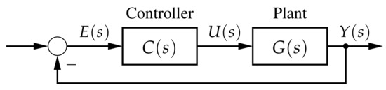
Figure 4.
Simplified structure of the closed control loop.
The transfer function of the (nominal) closed loop system using the plant Equation (4) and the controller Equation (6) can be expressed as follows
The second order system in Equation (7) is stable if and only if all coefficients of the denominator polynomial have the same sign (Stodola condition). The range of the controller parameters for which Equation (7) is stable is given by
Due to practical reasons, we shall use . Based on Ziegler–Nichols tuning method [29,31], the gain values and are obtained for the controller. The transient behavior of the controlled specimen for a reference deflection of 22 mm is shown Figure 5.
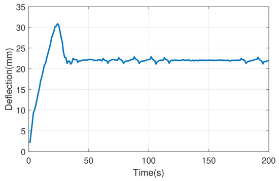
Figure 5.
Deflection of the controlled system for 22 mm reference with classically designed proportional integral (PI) controller.
5. Robust Control
5.1. Uncertainty Models
When the exact model of a physical system is not known due to for example unmodeled dynamics or nonlinearities, the unstructured uncertainty can be useful for modeling the errors. There are several types of unstructured uncertainty models in literature, e.g., [32,33,34]:
- Additive Uncertainty
- Multiplicative Uncertainty
- Feedback Uncertainty
- Multiplicative Feedback Uncertainty
In these models, denotes the transfer function of the nominal plant, is a proper and stable weight function characterizing the uncertainty dynamics, and contains the uncertainty, which can be an arbitrary stable transfer function fulfilling the inequality:
where
is the norm of the Hardy space . Additive uncertainty can be used when the numerator of the transfer function G contains uncertain terms while the feedback uncertainty is useful when the denominator has uncertainties. Also, multiplicative uncertainty is suitable for gain uncertainties. The block diagrams of these uncertainty models are shown in Figure 6.
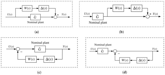
Figure 6.
Uncertainty models of the plant’s transfer function G(s). (a) Additive uncertainty; (b) Multiplicative uncertainty; (c) Feedback uncertainty; (d) Multiplicative feedback uncertainty.
Now, we want to describe the plant Equation (1) with these uncertainty models using the identified interval uncertainty Equation (2). With this extension we also cover nonlinearities such as hysteresis and other unmodeled dynamics. To do so, an appropriate weighting function W for each case should be found such that the condition in Equation (12) holds. First, we compute W for additive uncertainty case. Solving Equation (8) for the product term we get
In order to fulfill the bound in Equation (12) we replace the unknown parameters by their lower or upper bound as in Equation (2), respectively. A possible solution fulfilling the condition in Equation (12) is then given by
Applying the same procedure to other uncertainty models, the weighting function W and the uncertainty function can be described as follows:
- Multiplicative Uncertainty
- Feedback Uncertainty
- Multiplicative Feedback Uncertainty
As mentioned before, the transfer functions W and must be stable. In order to be stable, the transfer functions must also be proper, i.e., the degree of the numerator polynomial should not exceed the degree of the denominator polynomial. This structural condition is violated for the weighting function W of the feedback uncertainty model in Equation (18). Therefore, this model is not taken into account for the robust controller design.
5.2. Robust Stability Analysis
We assume that the controller was designed such that the closed loop with the nominal plant Equation (4) is stable. Let denote the corresponding (nominal) open loop transfer function, i.e.,
Furthermore, let us define and as the (nominal) sensitivity and complementary sensitivity function
Then, assuming an additive uncertainty Equation (8), the closed loop system is robustly stable if and only if
see [34]. The inequality Equation (22) can be adjusted into:
This condition can be interpreted graphically in the Nyquist diagramm: The envelope of the frequency response with the center and the radius cannot include or circumvent the critical point . Then, the closed loop system is stable because of the small gain theorem [32].
The other uncertainties have different versions of such conditions. Table 1 summarizes the robust stability conditions for the uncertainty models.

Table 1.
Robust stability conditions for different uncertainties [32,34].
5.3. Robust PI Control
A PI controller based on robust stability analysis is designed to investigate the effectiveness of the proposed design method. The (nominal) open loop transfer function of system in Equation (4) with the controller Equation (6) is expressed as
The (nominal) associated sensitivity and complementary sensitivity function are given by
By substituting the above equations in the robust stability condition of each uncertainty model, the range of the controller parameters for which the robust stability of the system is guaranteed can be obtained. To do so, the norms of auxiliary transfer functions occurring in the stability conditions of Table 1 are calculated and then plotted for different values of and as it is shown in Figure 7 and Figure 8. Note that for our model the auxiliary transfer functions resulting from the additive and multiplicative model are the same. The level sets of function values of the corresponding Hardy space norm less than one fulfill the conditions and ensure robust stability.
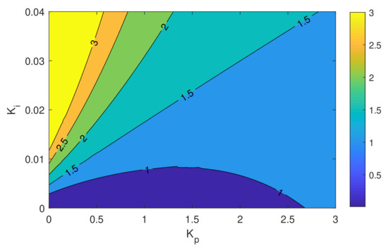
Figure 7.
Level sets of and for different values of and for the system with additive and multiplicative uncertainty.
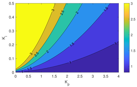
Figure 8.
Level sets of for different values of and for the system with multiplicative feedback uncertainty.
To verify the performance of the robust PI controller, output position control of the textile reinforced composite for a desired deflection was tested. The selected gain values considering the additive/multiplicative uncertainty are and . The Bode plot of the auxiliary transfer functions, and , is shown in Figure 9. Clearly, the magnitude plot stays below such that robust stability condition is fulfilled. The result of the experiment for a reference deflection of 22 mm is shown in Figure 10. It can be seen that the control action is really slow which is due to small value of the integral gain.
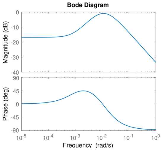
Figure 9.
Bode diagram of for and considering multiplicative uncertainty.
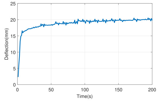
Figure 10.
Deflection of the controlled system with multiplicative uncertainty for 22 mm reference using a robust PI controller.
The same experiment was repeated for the feedback multiplicative uncertainty case using the gain values and . The Bode plot of the auxillary transfer function occurring in the stability condition using these gain values is shown in Figure 11. Experimental results in Figure 12 show that this controller has a better performance in comparison to other uncertainty models and classical controllers. It takes less time to reach the reference value. Furthermore, it provides stability for the whole set of plants described by Equation (11).
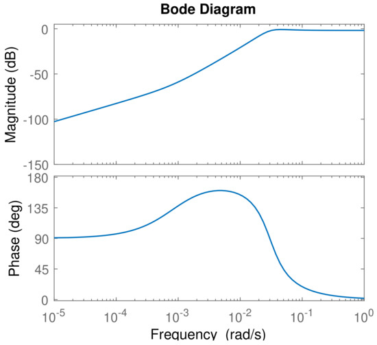
Figure 11.
Bode diagram of for and considering multiplicative feedback uncertainty.
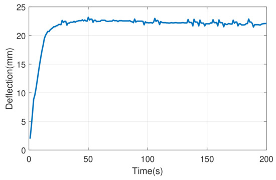
Figure 12.
Deflection of the controlled system with multiplicative feedback uncertainty for 22 mm reference using a robust PI controller.
6. Conclusions
In this paper, the mathematical model of a textile reinforced composite actuated by shape memory alloys is described using various unstructured uncertainty models. Through this model the nonlinearities of the system including hysteresis are covered. The robust stability analysis of the proposed model is carried out and a robust proportional–integral controller based on this analysis is designed. Among all uncertainty models, the multiplicative feedback uncertainty is best suited for the system. The experimental results show that the designed controller based on this uncertainty model has a better performance in stabilizing the composite at a desired deflection. It takes less time to reach the reference value and reduces the overshoot.
In the present case, the specimen was manufactured individually. We expect that active textile reinforced composites will be used more extensively in soft robotic applications and therefore be available in larger quantities in the future. We used very common electronic standard components to implement position control. The power consumption of typically less than 50W is hardly a limitation for practical applications.
Author Contributions
Conceptualization, K.R.; Methodology, K.R.; Software, N.K.; Validation, N.K.; Formal analysis, N.K. and K.R.; Investigation, N.K.; Writing—original draft preparation, N.K.; Writing—review and editing, K.R.; Visualization, N.K. and K.R.; Supervision, K.R.; Project administration, K.R.; Funding acquisition, K.R. All authors have read and agreed to the published version of the manuscript.
Funding
This research was funded by Deutsche Forschungsgemeinschaft (DFG, German Research Foundation), grant number Research Training Group 2430 “Interactive Fiber Rubber Composites”.
Acknowledgments
The authors would like to thank Dipl.-Ing. Klemens Fritzsche for interesting discussions which contributed to the paper.
Conflicts of Interest
The authors declare no conflict of interest.
References
- Hughes, J.; Culha, U.; Giardina, F.; Guenther, F.; Rosendo, A.; Iida, F. Soft manipulators and grippers: A review. Front. Robot. AI 2016, 3, 69. [Google Scholar] [CrossRef]
- Polygerinos, P.; Correll, N.; Morin, S.A.; Mosadegh, B.; Onal, C.D.; Petersen, K.; Cianchetti, M.; Tolley, M.T.; Shepherd, R.F. Soft robotics: Review of fluid-driven intrinsically soft devices; manufacturing, sensing, control, and applications in human-robot interaction. Adv. Eng. Mater. 2017, 19, 1700016. [Google Scholar] [CrossRef]
- Rus, D.; Tolley, M.T. Design, fabrication and control of soft robots. Nature 2015, 521, 467–475. [Google Scholar] [CrossRef] [PubMed]
- Siddika, A.; Al Mamun, M.A.; Alyousef, R.; Amran, Y.M. Strengthening of reinforced concrete beams by using fiber-reinforced polymer composites: A review. J. Build. Eng. 2019, 100798. [Google Scholar] [CrossRef]
- Naser, M.; Hawileh, R.; Abdalla, J. Fiber-reinforced polymer composites in strengthening reinforced concrete structures: A critical review. Eng. Struct. 2019, 198, 109542. [Google Scholar] [CrossRef]
- Mohammed, L.; Ansari, M.N.; Pua, G.; Jawaid, M.; Islam, M.S. A review on natural fiber reinforced polymer composite and its applications. Int. J. Polym. Sci. 2015, 2015, 243947. [Google Scholar] [CrossRef]
- Sohn, J.W.; Kim, G.W.; Choi, S.B. A state-of-the-art review on robots and medical devices using smart fluids and shape memory alloys. Appl. Sci. 2018, 8, 1928. [Google Scholar] [CrossRef]
- González García, C.; Meana Llorián, D.; Pelayo García-Bustelo, B.C.; Cueva Lovelle, J.M. A review about smart objects, sensors, and actuators. Int. J. Interact. Multimed. Artif. Intell. 2017, 4, 7–10. [Google Scholar] [CrossRef]
- Shian, S.; Bertoldi, K.; Clarke, D.R. Dielectric elastomer based “grippers” for soft robotics. Adv. Mater. 2015, 27, 6814–6819. [Google Scholar] [CrossRef] [PubMed]
- Jin, M.; Lee, J.; Ahn, K.K. Continuous nonsingular terminal sliding-mode control of shape memory alloy actuators using time delay estimation. IEEE/ASME Trans. Mechatronics 2014, 20, 899–909. [Google Scholar] [CrossRef]
- Jani, J.M.; Leary, M.; Subic, A.; Gibson, M.A. A review of shape memory alloy research, applications and opportunities. Mater. Des. 2014, 56, 1078–1113. [Google Scholar] [CrossRef]
- Sreekumar, M.; Nagarajan, T.; Singaperumal, M.; Zoppi, M.; Molfino, R. Critical review of current trends in shape memory alloy actuators for intelligent robots. Ind. Robot. Int. J. 2007, 34, 285–294. [Google Scholar] [CrossRef]
- Tanaka, K.; Nagaki, S. A thermomechanical description of materials with internal variables in the process of phase transitions. Ingenieur-Archiv 1982, 51, 287–299. [Google Scholar] [CrossRef]
- Liang, C.; Rogers, C.A. One-dimensional thermomechanical constitutive relations for shape memory materials. J. Intell. Mater. Syst. Struct. 1997, 8, 285–302. [Google Scholar] [CrossRef]
- Brinson, L.C. One-dimensional constitutive behavior of shape memory alloys: Thermomechanical derivation with non-constant material functions and redefined martensite internal variable. J. Intell. Mater. Syst. Struct. 1993, 4, 229–242. [Google Scholar] [CrossRef]
- Preisach, F. Über die magnetische Nachwirkung. Z. Phys. 1935, 94, 277–302. [Google Scholar] [CrossRef]
- Brokate, M.; Sprekels, J. Hysteresis operators. In Hysteresis and Phase Transitions; Springer: Berlin/Heidelberg, Germany, 1996; pp. 22–121. [Google Scholar]
- Al Janaideh, M.; Rakheja, S.; Su, C.Y. A generalized Prandtl–Ishlinskii model for characterizing the hysteresis and saturation nonlinearities of smart actuators. Smart Mater. Struct. 2009, 18, 045001. [Google Scholar] [CrossRef]
- Ljung, L. Perspectives on system identification. Annu. Rev. Control. 2010, 34, 1–12. [Google Scholar] [CrossRef]
- Isermann, R.; Münchhof, M. Identification of Dynamic Systems—An Introduction with Applications; Springer: Berlin/Heidelberg, Germany, 2011. [Google Scholar]
- Keshtkar, N.; Röbenack, K.; Fritzsche, K. Position Control of Textile-Reinforced Composites by Shape Memory Alloys. In Proceedings of the 2019 23rd International Conference on System Theory, Control and Computing (ICSTCC), Sinaia, Romania, 9–11 October 2019; pp. 442–447. [Google Scholar]
- Cherif, C.; Hickmann, R.; Nocke, A.; Schäfer, M.; Röbenack, K.; Wießner, S.; Gerlach, G. Development and testing of controlled adaptive fiber-reinforced elastomer composites. Text. Res. J. 2018, 88, 345–353. [Google Scholar] [CrossRef]
- STMicroelectronics. L298; Dual Full-Bridge Driver–Datasheet; STMicroelectronics: Geneva, Switzerland, 2000. [Google Scholar]
- Sharp. GP2Y0A41SK0F, Distance MEasuring Sensor Unit, Measuring Distance: 4 to 30 Cm, Analog Output Type; Datasheet; Sharp: Osaka, Japan, 2011; Available online: https://global.sharp/products/device/lineup/data/pdf/datasheet/gp2y0a41sk_e.pdf (accessed on 14 January 2020).
- Röbenack, K. Mobile Robotics with Arduino: Design and Programming; CreateSpace Independent Publishing Platform: Scotts Valley, CA, USA, 2018. [Google Scholar]
- Kurniawan, A. Getting Started with Matlab Simulink and Arduino; PE Press: Prešov, Slovakia, 2013. [Google Scholar]
- Hespanha, J.P. Linear Systems Theory, 2nd ed.; Princeton University Press: Princeton, NJ, USA; Exford, UK, 2018. [Google Scholar]
- Ljung, L. System Identification Toolbox™; The MathWorks, Inc.: Natick, MA, USA, 2012. [Google Scholar]
- O’Dwyer, A. Handbook of PI and PID cOntroller Tuning Rules; Imperial College Press: London, UK, 2009. [Google Scholar]
- Datta, A.; Ho, M.T.; Bhattacharyya, S.P. Structure and Synthesis of PID Controllers; Springer: London, UK, 2000. [Google Scholar]
- Franklin, G.F.; Powell, J.D.; Workman, M.L. Digital Control of Dynamic Systems, 3rd ed.; Addison-Wesley: Menlo Park, CA, USA, 1998. [Google Scholar]
- Zhou, K.; Doyle, J.C. Essentials of Robust Control; Prentice Hall: Upper Saddle River, NJ, USA, 1998. [Google Scholar]
- Matušů, R.; Prokop, R.; Pekař, L. Parametric and unstructured approach to uncertainty modeling and robust stability analysis. Int. J. Math. Model. Methods Appl. Sci. 2011, 5, 1011–1018. [Google Scholar]
- Reinschke, K. Lineare Regelungs- und Steuerungstheorie, 2nd ed.; Springer: Berlin/Heidelberg, Germany, 2014. (In German) [Google Scholar]
© 2020 by the authors. Licensee MDPI, Basel, Switzerland. This article is an open access article distributed under the terms and conditions of the Creative Commons Attribution (CC BY) license (http://creativecommons.org/licenses/by/4.0/).