Predictive Path Following and Collision Avoidance of Autonomous Connected Vehicles


1
The Institute of Cartography and Geoinformatics, University of Hannover, D-30167 Hannover, Germany
2
Institute of Geodesy, University of Hannover, D-30167 Hannover, Germany
*
Author to whom correspondence should be addressed.
Algorithms 2020, 13(3), 52; https://doi.org/10.3390/a13030052
Submission received: 20 January 2020
/
Revised: 25 February 2020
/
Accepted: 26 February 2020
/
Published: 28 February 2020
(This article belongs to the Special Issue Algorithms for Reliable Estimation, Identification and Control)
Abstract
:This paper considers nonlinear model predictive control for simultaneous path-following and collision avoidance of connected autonomous vehicles. For each agent, a nonlinear bicycle model is used to predict a sequence of the states and then optimize them with respect to a sequence of control inputs. The objective function of the optimal control problem is to follow the planned path which is represented by a Bézier curve. In order to achieve collision avoidance among the networked vehicles, a geometric shape must be selected to represent the vehicle geometry. In this paper, an elliptic disk is selected for that as it represents the geometry of the vehicle better than the traditional circular disk. A separation condition between each pair of elliptic disks is formulated as time-varying state constraints for the optimization problem. Driving corridors are assumed to be also Bézier curves, which could be obtained from digital maps, and are reformulated to suit the controller algorithm. The algorithm is validated using MATLAB simulation with the aid of ACADO toolkit.
1. Introduction
Autonomous driving has gained a lot of attention in the last decade, from both industry and academia, due to its anticipated impacts on the enhancement of traffic efficiency. There are many types of controllers that can be used for autonomous driving. In [1], sensitivity analysis is used to design an automatic path following controller by means of an automatic modification of desired output trajectories. A novel path planning algorithm is presented in [2] for planning and execution of heavy multi-body vehicles with multi-axle steering. Sliding mode control is used in [3] for trajectory tracking and control of autonomous high-speed ground vehicles.
Nonlinear Model Predictive Control (NMPC) has proven successful results and has been employed in many recent publications [4,5] because it combines both control and collision avoidance into one algorithm which can be used for critical maneuvers. It is an optimization-based controller that has been widely used for various transportation systems such as autonomous ships [6] and autonomous vehicles [4]. It is mainly used for two famous problems: Trajectory tracking and path following. Recently, it started to get attention to be used for collision avoidance because of its ability to handle nonlinear constraints [7]. In [8], NMPC is used for the trajectory tracking of a scaled autonomous racing car with a higher level planner to account for collision avoidance by building local approximations of the controls from linearized time-varying models. A bi-level NMPC is developed in [9] for intersection scenarios to allocate and update optimal and collision-free timeslots when each vehicle is allowed to occupy the intersection, and provide optimal actuation commands given the allocated timeslots using another low level controller. Experimental validation of NMPC is given in [4] to show that online nonlinear optimization tools are efficient for real-time applications on hardware with limited processing resources, and a comparison of different embedded nonlinear optimization algorithms for autonomous vehicle control is provided. In [10], a legible model predictive control scheme is presented for overtaking of autonomous vehicles on highways in order to enhance the safety and improve the efficiency.
It has been shown recently in [11] that NMPC can meet the safety and robustness requirements of autonomous systems by demonstrating some real world scenarios of autonomous driving under consideration of unknown obstacles. The issue of critical maneuvers of autonomous vehicles is discussed in [12], where a real-time trajectory planning is achieved using model predictive control employing homotopic classes to avoid the computation complexity of sophisticated models.
The main contribution of this work is to fill the gap in NMPC algorithms for autonomous driving by employing paths and road corridors that could be obtained directly from existing digital maps.
This paper is organized as follows. Section 2 describes the vehicle model employed by NMPC, the generation of the reference trajectory, and clarifies the control objective. The controller synthesis is presented in Section 3: A brief introduction of NMPC is given first for the trajectory tracking of the vehicle, followed by how to utilize state and control constraints for comfort driving. After that, the development of the collision avoidance constraints is presented, followed by some guidelines for the implementation of the dynamic optimization problem and the software used for that. MATLAB-based simulation results are given in Section 4. Section 5 concludes this paper and provide our outlook for future work.
2. Problem Formulation
2.1. Vehicle Modeling
Nonlinear Model Predictive Control (NMPC) employs a vehicle dynamic model in order to predict the future trajectory of the vehicle over a predefined prediction horizon. This model is the key for a successful vehicle control system. In the literature of vehicle control, there are different models of vehicles varying in the complexity from kinematic to complex kinetic models [13]. While kinetic models provide accurate prediction of the vehicle motion, they might increase the complexity in the design of collision avoidance systems, and require, during the deployment, high computation time and small sampling interval. It has been shown in the literature that the kinematic model can provide reasonable accuracy by adding constraints on the rate of change of the inputs to be consistent with the low level controllers of the vehicle [14,15]. Therefore, the state space representation of the nonlinear kinematic bicycle model [16]
is used in this paper, where indicates the position of the center of gravity (CG) of the vehicle, is the longitudinal velocity, is the heading angle of the vehicle, is the side-slip angle between the velocity vector and the longitudinal direction of the vehicle, is the longitudinal acceleration input used to control the velocity, is the steering angle, L is the wheelbase, and is the distance between CG and the rear wheel (see Figure 1).
In order to achieve consistency between the kinematic model and the real vehicle model, interval constraints on the control inputs and their rate of change must be imposed. These constraints play a key role in achieving comfort driving and avoids extreme driving conditions by limiting the maximum and minimum value for the longitudinal acceleration and steering angle inputs. The maximum/minimum longitudinal acceleration can be obtained experimentally and vary from one vehicle to the other based on the engine size. The steering angle can be limited in terms of a maximum safe lateral acceleration to achieve normal driving behavior and avoid extreme slipping [14]. Therefore, the acceleration and steering angle constraints
must be considered. Constraints on time derivative of the control inputs are beneficial for avoiding jerky behavior, and are represented in the model by the augmentation of the control inputs, , as extra states and define the rate of change as a new virtual inputs, , as
Therefore, the rate of change constraints are formulated as
Based on that, a compact state-space model of the system is
where , is the state vector, , , is the control input vector, and is a continuously differentiable function.
2.2. The Path-Following Problem
In the domain of vehicle steering control, there are two common techniques: Trajectory tracking and path following. In trajectory tracking problems, time and space reference are provided to the controller and the vehicle may accelerate/decelerate in order to compensate for the tracking error. Considering our vehicle model (5), the objective of the trajectory tracking is to design a controller that steers the system states to follow a time-dependent reference trajectory and therefore the tracking error is [17].
The path following problem is handled differently as the controller objective is to steer the vehicle to be geometrically on a certain path while maintaining a reference speed, and without adding strict requirements when to be where on this path [18]. Consider a path curve
which is parameterized by the function , where is the time-dependent path parameter whose time evolution is not specified. The objective of the controller is to choose the system input and the timing such that the path is followed as exactly as possible.
Given the vehicle state space Model (5), which is assumed to have an output function , and the Path (6), the path following objective could be represented as:
- Path Convergence: The system output converges to the set , i.e.,:
- Monotonous Forward Motion: The system moves along in the direction of increasing values of , i.e., and .
2.3. Map Representation Using Bézier Curves
Two of the necessary requirements of any autonomous driving controller is the ability to handle the road boundaries generated from digital maps and have a path representation that could be followed by the motion controller.
In [19], an automatic procedure for generating driving boundaries from OpenStreetMap is presented, which expands its original representation, replacing polylines by polynomial-based roads, whose sections are defined using Bézier curves. This method has been validated successfully on a peri-urban environment without any human intervention. Therefore, we assume that the road is represented by polynomials whose sections are defined using Bézier curves. The road corridor is represented by two Bézier curves, one for the left boundary and the other for the right one. The path that should be follow by the vehicle, which is assumed to be the at the center of the lane is represented also by a Bézier curve.
Bézier curves [20] have recently attracted many researchers for digital map representation for autonomous driving [19]. They are defined as
where n is the order of the polynomial, are the control points defining the curvature of the curve (see Figure 2), and the Bernstein coefficients given by
with .
Depending on the Bézier polynomial degree, it would be possible to define any arbitrary road as one Bézier curve. However, higher degrees of the polynomial leads to high computation time and difficulties in calculating the control points. Moreover, for the purpose of autonomous driving, defining the whole road in just one huge polynomial is not required and makes the control problem intractable. Therefore, the common approach in computer graphics is to define complex paths by concatenating quadratic and cubic curves, taking into consideration the continuity constraints [19]. The overall control problem is to utilize the kinematic bicycle Model (5) to design a controller that follows the planned reference path defined by a Bézier Curve (7) and avoid collision with nearby objects, that are assumed to be connected with our own vehicle, by doing necessary maneuvers. The controller should be able to respect the road boundaries or corridor which are also assumed to be represented by a left and right Bézier curves.
3. Controller Synthesis
3.1. Nonlinear Predictive Path-Following Control
Nonlinear Model Predictive Control (NMPC), also known as Receding Horizon Control and Moving Horizon Optimal Control, is a famous control technique for vehicle control systems that has roots in optimal control. It has been widely adopted in industry as an effective way to deal with multi-variable constrained control problems [21]. The basic concept of MPC is to optimize the forecast of the system, generated by a nominal dynamic model, and optimize it to produce the best decision, i.e., the control signal at the current time slot, while planning the nominal future control actions. This is achieved by employing the prediction of the system model to formulate and solve a dynamic optimization problem online where tracking errors, namely the difference between the predicted output and the desired reference, is minimized over a future horizon, possibly subject to constraints on the control inputs (the manipulated variables) and the states. These constraints could be nonlinear and time-varying over the prediction horizon.
This optimization problem is solved in discrete control intervals suitable for the system dynamics. At each step, the MPC algorithm computes an open-loop sequence of control input adjustments. The first input in the optimal sequence is injected into the system, and the entire optimization is repeated for the subsequent control intervals.
Consider a nonlinear state space Model (5) with and subject to generic state and control constraints
where and define the admissible state and control sets, respectively. These admissible sets will be designed later to achieve comfort driving, respect physical constraints of the vehicle, and perform collision avoidance.
In order to include the Path (6) into the control problem, we treat its parameter as an extra virtual state whose time evolution is controlled by an extra virtual input [18]. Therefore, an additional differential equation
is added to the system where is the extra state that represents the path time evolution, and is the virtual control input that adds an extra degree of freedom in the controller design.
The optimal control problem (OCP) of the NMPC used for path following will be
where is the stage cost given by a positive definite function, is the prediction horizon, is the admissible set for the path parameter, and is the admissible set for the path timing law. The stage cost function for the path following problem of the autonomous vehicle could be defined as
Here, is positive semi-definite matrix, is strictly positive-definite, is the output function for the vehicle state space Model (5) and is defined as: , and
is the reference path which is defined using quadratic Bézier curves.
3.2. Collision Avoidance
In order to account for collision avoidance of nearby vehicles, an NMPC is employed, due to its ability to handle time-varying nonlinear constraints by adding coupling constraints to the vehicle optimization problem with its neighbors to guarantee that the solution of the OCP provides a collision-free trajectory. The vehicles are assumed to be connected and they are exchanging information about their future predictions.
Consider encountered vehicles indexed by a superscript , for instance, the state vector of each neighbor is denoted by . Each of them is represented geometrically by an elliptic disk (see Figure 3) which is parameterized by the center position , orientation (heading angle) , semi-major radius , and semi-minor radius . The elliptic disk is the closed type of conic section results from the intersection of a cone by a plane, and is expressed as
where is the 3-D column vector containing the homogeneous coordinates,
, , and .
Based on that, the collision avoidance is formulated in terms of coupling state constraints that represent the separation condition between the moving elliptic disk of the vehicle and the neighbor vehicle . In the following, we recall a proposition that formulates the collision avoidance constraints.
Proposition 1.
Consider a pair of moving elliptic disksin the Euclidean planerepresented by the matrices and, respectively. Letbe their characteristic polynomial anddenote the discriminant ofwith respect to λ. Suppose that every pairis separate, then the motions of them are collision-free for allif
- ,
Proof.
See [17]. ☐
3.3. Road Corridor Respect
In this subsection, we develop the sufficient constraints that could be added to the optimization Problem (11) to guarantee our vehicle respect the driving corridors, generated from digital maps, in all the maneuvering. As for the reference path, it is assumed that we get two Bézier curves from the map; one for the left boundary and the other for the right one. Explicit representations of Bézier Curves (7) are not suitable for formulating the nonlinear constraints, and therefore we want to turn (7) into an implicit curve equation, that is one where we have no dependence on the parameter , i.e., . This can be done using the resultant (or the Bézout’s determinant). The advantage is that holds for points on one side of the Bézier curve, and for those on the other side. As a result, we get the following representation for quadratic curves [20]:
where , and . The right and left boundary constraints are and , respectively.
3.4. Optimization Problem Implementation
In order to utilize the aforementioned infinite dimensional OCP of the NMPC, a proper formulation of the optimization problem implementation is required. There are two possible categories when it comes to dynamic optimization problems; indirect and direct methods. Indirect methods, such as calculus of variations and dynamic programming, consider the continuous NMPC as it is and does not require discretization of the problem. They provide exact analytic solution of the optimal control problem [22], but they are not common to be used for nonlinear optimal control problems due to their inability to handle a wide class of systems because they require a guess of the optimal control structure [22].
Direct methods, such as collocation [23] and multiple shooting [24], are the most desirable technique for formulating and parameterizing NMPC optimization problem. The main idea behind them is introducing the discretization and finite parameterization into the optimal control problem formulation which results in a Nonlinear Programming Problem (NLP), and then solve it directly with numerical methods. In the multiple shooting technique, the one used in this paper, the nonlinear continuous ordinary differential equation (ODE) and the OCP are discretized at a proper sampling interval [24].
Consider a general OCP of the form
where is the ODE model of the system, is the initial condition, and is a vector function which represents the optimization state and control constraints. The control input is discretized at the time instants
such that
The nonlinear ODE, which can not be solved analytically, must be solved numerically on each subinterval using a suitable integration technique, e.g., fourth-order Runge–Kutta, and starting with an artificial initial value . The trajectory pieces are obtained by solving the initial value problem (IVP)
as function of and , and also and compute numerically the integral
Based on that, the NLP formulation of Problem (14) is represented as
where (16b) represents the initial condition, Equation (16c) represents the continuity condition between each two consecutive subintervals, Equations (16d) and (16e) represent the discretized constraints, and is the solution of the IVP (15). The NLP (16) is solved using sequential quadratic programming (SQP), with the aid of the method of Lagrange multipliers where the Hessian matrix is approximated using Gauss–Newton [25]. Each quadratic problem (QP) is then solved using active-set method [26].
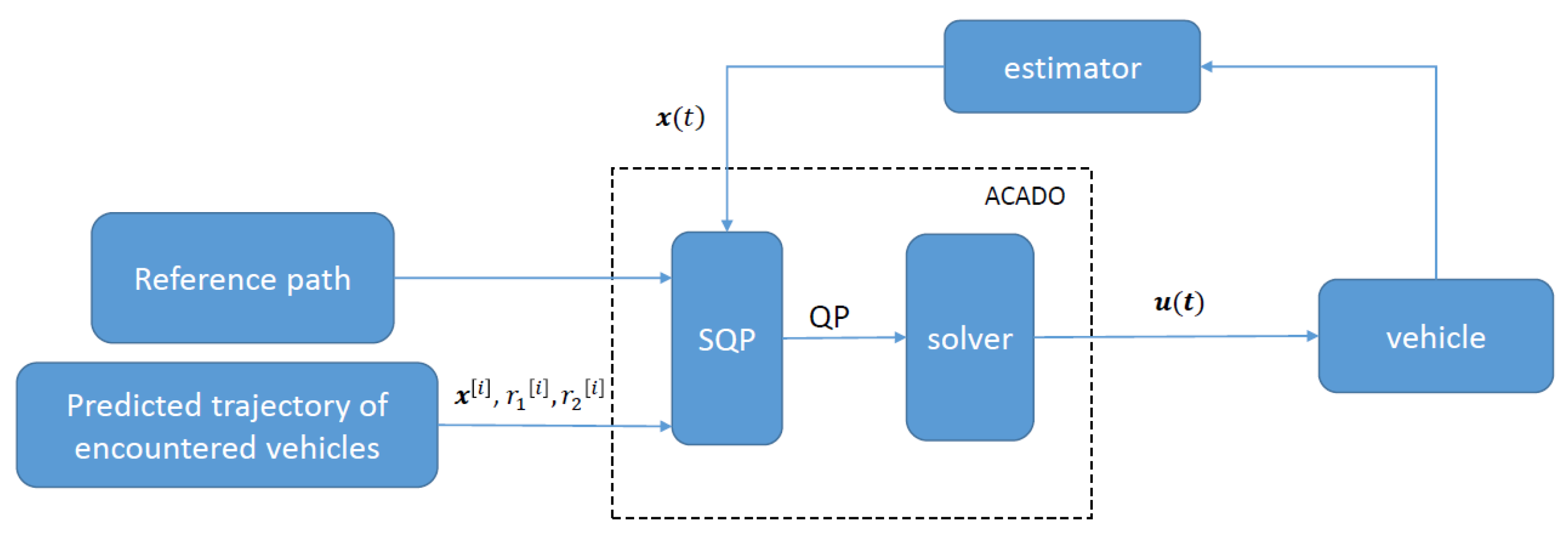
The open-source ACADO Code Generation toolkit [26] is used in the implementation of the NMPC algorithm. Based on a symbolic representation of optimal control problems, ACADO generates an optimized and self-contained C code for the SQP formulation with static memory for a good real-time performance. The C code can be integrated into MATLAB as MATLAB executable (mex) files.
The main steps of the implementation are briefly described as follows:
- The continuous state space model is symbolically defined using C-code or the MATLAB interface, then it is simplified employing automatic differentiation tools and using zero entries in the Jacobian matrix. The result is an efficient real time C-code for the integration of the continuous nonlinear system which will be used for the prediction.
- The optimization problem cost function and constraints are symbolically defined, parametrized by the aforementioned direct multiple shooting technique, and the resulting, large but sparse, Quadratic Problem (QP) is condensed.
- The discretized QP is then solved using qpOASES solver.
A representation of the usage of NMPC for path-following and collision avoidance is shown in Figure 4, and Algorithm 1 describes the NMPC usage as follows.
| Algorithm 1 NMPC Algorithm for Path Following. |
| 1: Set the time index , the sampling interval , the prediction horizon , weight matrices Q and R. |
| 2: Measure the values of the states or estimate them. |
| 3: Solve the optimization Problem (16) over the discrete time instants and get the optimal control sequence and the corresponding predicted states . |
| 4: Apply only the first control element . |
| 5: wait for the next sample and set the time index , then go to step 2. |
Remark 1.
There are many state estimation techniques in the literature that could be used to get the state vector. A survey for these techniques is given in [27].
4. Simulation Results
In this section, simulation results are presented to demonstrate the validity and assess the performance of the proposed NMPC scheme for path-following and collision avoidance of autonomous vehicles. Simulation is done in MATLAB 2017b using the static C-code generated from the ACADO toolkit [26]. These results have been obtained on a GHz core i5 CPU with 16 GB RAM. In the simulation scenario, there are two vehicles; the own vehicle and the encountered one. It is assumed that the encountered vehicle has the priority and therefore its collision avoidance algorithm was not triggered, and it sends its future prediction states to the own vehicle. In Table 1, the parameters of the vehicle Model (1), which are obtained from [28], and the NMPC parameters are given.
The vehicle starts from the initial position and the NMPC steers it to follow the reference quadratic Bézier path with the control points , , and As shown in Figure 5, the NMPC steers the vehicle to follow the reference path, and when the slower vehicle impedes this path, the NMPC steers the vehicle to avoid collision with the encountered vehicle by overtaking it, while respecting the control input constraints and the road corridors. In Figure 6a, it is shown that the vehicle could achieve the desired speed except during the collision avoidance maneuvering. It is clear in Figure 6e,f that maneuvering of the vehicle does not have any abrupt change in the steering angle and therefore it is consistent with the steering system dynamics. In Figure 6c,d, it is shown that the maximum allowed acceleration is obeyed while avoiding any jerky actions due to the constraints on the acceleration rate of change. The distance between the centers of both vehicles at the closest point of approach is about which is quite smaller compared to selecting circular disks, as presented in [14], which gives a minimum distance of at least . The maximum execution time of the presented scheme is about which qualifies it to be used for experimental evaluation, and the maximum number of iterations is 100.
5. Conclusions
An NMPC scheme is presented in this paper for the problem of path-following of autonomous vehicles with integrated collision avoidance based on ellipse geometry. A bicycle model is used with both acceleration and steering angle as control inputs. Employing a quadratic cost function that penalizes the deviation from the path, a dynamic optimization problem is formulated with linear inequality state and control constraints to achieve comfort driving. Collision avoidance is achieved by adding nonlinear time-varying state constraints based on the separation condition between elliptic disks. To guarantee staying within the road boundaries, implicit Bézier constraints are added to the OCP. The optimization problem is parametrized and solved using ACADO toolkit and is evaluated on MATLAB platform. The NMPC shows good performance for following of the predefined path while avoiding jerky behavior and collision with nearby vehicles.
Our future aim is to increase the safety levels of the presented scheme by considering robust NMPC techniques for uncertain nonlinear models. The upper bound of the path-following error is parametrized with the aid of an auxilary control law, and then included into the optimization problem as a decision variable to make it as small as possible. Moreover, a maximum permissible error could be added as a reference to the optimization problem.
Author Contributions
Methodology, M.A.; Writing—original draft preparation, M.A. and S.S.; Writing—review and editing, M.A. and S.S.; Supervision, S.S.; All authors have read and agreed to the published version of the manuscript.
Funding
This research was funded by the German Research Foundation (DFG) as a part of the Research Training Group Integrity and Collaboration in dynamic SENSor networks (i.c.sens) [GRK2159].
Conflicts of Interest
The authors declare no conflict of interest.
References
- Rauh, A.; Kersten, J.; Auer, E.; Aschemann, H. Sensitivity-based feedforward and feedback control for uncertain systems. Computing 2012, 94, 357–367. [Google Scholar] [CrossRef]
- Beyersdorfer, S.; Wagner, S. Novel model based path planning for multi-axle steered heavy load vehicles. In Proceedings of the 16th International IEEE Conference on Intelligent Transportation Systems (ITSC 2013), The Hague, The Netherlands, 6–9 October 2013; pp. 424–429. [Google Scholar] [CrossRef]
- Wang, J.; Steiber, J.; Surampudi, B.; Member, S. Autonomous Ground Vehicle Control System for High-Speed and Safe Operation. In Proceedings of the American Control Conference, Seattle, WA, USA, 11–13 June 2008; pp. 218–223. [Google Scholar]
- Quirynen, R.; Berntorp, K.; Cairano, S.D. Embedded Optimization Algorithms for Steering in Autonomous Vehicles based on Nonlinear Model Predictive Control. In Proceedings of the Annual American Control Conference (ACC), Milwaukee, WI, USA, 27–29 June 2018; pp. 3251–3256. [Google Scholar] [CrossRef]
- Abbas, M.A.; Milman, R.; Eklund, J.M. Obstacle Avoidance in Real Time with Nonlinear Model Predictive Control of Autonomous Vehicles. Can. J. Electr. Comput. Eng. 2017, 40, 12–22. [Google Scholar] [CrossRef]
- Abdelaal, M. Nonlinear Model Predictive Control for Trajectory Tracking and Collision Avoidance of Surface Vessels. Ph.D. Thesis, University of Oldenburg, Oldenburg, Germany, 2018. [Google Scholar] [CrossRef]
- Pereira, G.C. Model Predictive Control for Autonomous Driving of Over-Actuated Research Vehicle. Ph.D. Thesis, KTH Royal Institute of Technology, Stockholm, Sweden, 2016. [Google Scholar]
- Liniger, A.; Domahidi, A.; Morari, M. Optimization-based autonomous racing of 1: 43 scale RC cars. Optim. Control Appl. Methods 2015, 36, 628–647. [Google Scholar] [CrossRef] [Green Version]
- Hult, R.; Zanon, M.; Gros, S.; Falcone, P. Optimal Coordination of Automated Vehicles at Intersections: Theory and Experiments. In Proceedings of the European Control Conference, Naples, Italy, 25–28 June 2019. [Google Scholar] [CrossRef]
- Brüdigam, T.; Ahmic, K.; Leibold, M.; Wollherr, D. Legible Model Predictive Control for Autonomous Driving on Highways. IFAC-PapersOnLine 2018, 51, 215–221. [Google Scholar] [CrossRef]
- Rick, M.; Clemens, J.; Sommer, L.; Folkers, A.; Schill, K.; Büskens, C. Autonomous Driving Based on Nonlinear Model Predictive Control and Multi-Sensor Fusion. IFAC-PapersOnLine 2019, 52, 182–187. [Google Scholar] [CrossRef]
- Yi, B.; Bender, P.; Bonarens, F.; Stiller, C. Model Predictive Trajectory Planning for Automated Driving. IEEE Trans. Intell. Veh. 2018, 4, 24–38. [Google Scholar] [CrossRef]
- Rajamani, R. Vehicle Dynamics and Control; Springer: Berlin, Germany, 2006; p. 470. [Google Scholar]
- Alrifaee, B. Collision Avoidance Networked Model Predictive Control for Vehicle Collision Avoidance. Ph.D. Thesis, RWTH Aachen University, Aachen, Germany, 2017. [Google Scholar] [CrossRef]
- Polack, P.; Altché, F.; D’Andréa-Novel, B.; De La Fortelle, A. Guaranteeing Consistency in a Motion Planning and Control Architecture Using a Kinematic Bicycle Model. In Proceedings of the American Control Conference, Milwaukee, WI, USA, 27–29 June 2018; pp. 3981–3987. [Google Scholar] [CrossRef] [Green Version]
- Guanetti, J.; Kim, Y.; Borrelli, F. Control of connected and automated vehicles: State of the art and future challenges. Annu. Rev. Control 2018, 45, 18–40. [Google Scholar] [CrossRef] [Green Version]
- Abdelaal, M.; Schön, S. Distributed Nonlinear Model Predictive Control for Connected Vehicles Trajectory Tracking and Collision Avoidance with Ellipse Geometry. In Proceedings of the 32nd International Technical Meeting of the Satellite Division of The Institute of Navigation (ION GNSS+ 2019), Miami, FL, USA, 16–20 September 2019; pp. 2100–2111. [Google Scholar]
- Faulwasser, T.; Matschek, J.; Zometa, P.; Findeisen, R. Predictive path-following control: Concept and implementation for an industrial robot. In Proceedings of the IEEE International Conference on Control Applications, Hyderabad, India, 28–30 August 2013; pp. 128–133. [Google Scholar] [CrossRef]
- Godoy, J.; Artuñedo, A.; Villagra, J. Self-Generated OSM-Based Driving Corridors. IEEE Access 2019, 7, 20113–20125. [Google Scholar] [CrossRef]
- Borrelli, H.; Boehm, W.; Paluszny, M. Bézier and B-Spline Techniques; Springer: Berlin, Germany, 2002. [Google Scholar]
- Rubagotti, M.; Raimondo, D.M.; Ferrara, A.; Magni, L. Robust model predictive control with integral sliding mode in continuous-time sampled-data nonlinear systems. IEEE Trans. Autom. Control 2011, 56, 556–570. [Google Scholar] [CrossRef] [Green Version]
- Borrelli, F.; Bemporad, A.; Morari, M. Explicit Nonlinear Model Predictive Control: Theory and Applications; Springer: Berlin, Germany, 2012. [Google Scholar]
- Tsang, T.; Himmelblau, D.; Edgar, T. Optimal control via collocation and nonlinear programming. Int. J. Control 1975, 21, 763–768. [Google Scholar] [CrossRef]
- Bock, H.G.; Plitt, K.J. Multiple Shooting Algorithm for Direct Solution of Optimal Control Problems. In Proceedings of the 9th IFAC World Congress, Budapest, Hungary, 2–6 July 1984; Elsevier: Budapest, Hungary, 1985; Volume 17, pp. 1603–1608. [Google Scholar] [CrossRef]
- Bock, H.G. Recent Advances in Parameter identification Techniques for O.D.E. In Numerical Treatment of Inverse Problems in Differential and Integral Equations: Progress in Scientific Computing; Birkhäuser: Basel, Sweden, 1983; Volume 2, pp. 95–121. [Google Scholar] [CrossRef]
- Houska, B.; Ferreau, H.J.; Diehl, M. ACADO toolkit-An open-source framework for automatic control and dynamic optimization. Optim. Control Appl. Methods 2011, 32, 298–312. [Google Scholar] [CrossRef]
- Jin, X.; Yin, G.; Chen, N. Advanced estimation techniques for vehicle system dynamic state: A survey. Sensors 2019, 19, 1–26. [Google Scholar] [CrossRef] [PubMed] [Green Version]
- Kong, J.; Pfeiffer, M.; Schildbach, G.; Borrelli, F. Kinematic and Dynamic Vehicle Models for Autonomous Driving Control Design. In Proceedings of the IEEE Intelligent Vehicles Symposium (IV), Seoul, Korea, 28 June–1 July 2015 ; pp. 2–7. [Google Scholar]
Figure 1.
Kinematic bicycle model of the vehicle.

Figure 2.
Bézier Curve (cubic, ).

Figure 3.
Elliptic Disk.

Figure 4.
Representation of Nonlinear Model Predictive Control (NMPC) usage for path following and collision avoidance.
Figure 4.
Representation of Nonlinear Model Predictive Control (NMPC) usage for path following and collision avoidance.

Figure 5.
Simulation results for collision avoidance in an overtaking scenario.

Figure 6.
Simulation results.


Table 1.
Vehicle and NMPC parameters.
© 2020 by the authors. Licensee MDPI, Basel, Switzerland. This article is an open access article distributed under the terms and conditions of the Creative Commons Attribution (CC BY) license (http://creativecommons.org/licenses/by/4.0/).
Share and Cite
MDPI and ACS Style
Abdelaal, M.; Schön, S. Predictive Path Following and Collision Avoidance of Autonomous Connected Vehicles. Algorithms 2020, 13, 52. https://doi.org/10.3390/a13030052
AMA Style
Abdelaal M, Schön S. Predictive Path Following and Collision Avoidance of Autonomous Connected Vehicles. Algorithms. 2020; 13(3):52. https://doi.org/10.3390/a13030052
Chicago/Turabian StyleAbdelaal, Mohamed, and Steffen Schön. 2020. "Predictive Path Following and Collision Avoidance of Autonomous Connected Vehicles" Algorithms 13, no. 3: 52. https://doi.org/10.3390/a13030052
Note that from the first issue of 2016, this journal uses article numbers instead of page numbers. See further details here.