Not So Robust after All: Evaluating the Robustness of Deep Neural Networks to Unseen Adversarial Attacks

Abstract

Deep neural networks (DNNs) have gained prominence in various applications, but remain vulnerable to adversarial attacks that manipulate data to mislead a DNN. This paper aims to challenge the efficacy and transferability of two contemporary defense mechanisms against adversarial attacks: (a) robust training and (b) adversarial training. The former suggests that training a DNN on a data set consisting solely of robust features should produce a model resistant to adversarial attacks. The latter creates an adversarially trained model that learns to minimise an expected training loss over a distribution of bounded adversarial perturbations. We reveal a significant lack in the transferability of these defense mechanisms and provide insight into the potential dangers posed by $L_{\infty }$-norm attacks previously underestimated by the research community. Such conclusions are based on extensive experiments involving (1) different model architectures, (2) the use of canonical correlation analysis, (3) visual and quantitative analysis of the neural network’s latent representations, (4) an analysis of networks’ decision boundaries and (5) the use of equivalence of $L_2$ and $L_{\infty }$ perturbation norm theories.

1. Introduction

The growth of computing power and data availability has led to the development of more efficient pattern recognition techniques, such as neural networks and deep learning. When a sample accurately represents a population of data and is of sufficient size, deep learning methods can produce impressive results, even on unseen data, making them suitable for tasks such as classification and prediction tasks. Although these methods offer significant advantages, they also come with limitations, such as the sensitivity of deep neural networks (DNNs) to data quality and sources, as well as overfitting when trained on insufficient amounts of data. However, variations in input samples from different domains or insufficient training data can still significantly affect the performance of DNNs. As DNNs are increasingly being employed in critical applications such as medicine and transportation, enhancing their robustness is essential due to the potentially severe consequences of their unpredictability.

Using adversarial attacks is one approach to examining DNNs’ robustness to diverse inputs. Adversarial attacks aim to generate the smallest adversarial perturbation, i.e., a change in input, that results in a misclassification by the model.

This study investigated the abilities and drawbacks of modern defense techniques against adversarial attacks, such as adversarial and robust training. The latter refers to the hypothesis proposed by Ilyas et al. [1]. It states that adversarial attacks exploit non-robust features inherent to the data set rather than the objects in the images. According to this hypothesis, removing these features from the data set and training a model on the modified data should render adversarial attacks ineffective.

We expanded the experiments from the original paper, trained a model on robust features, and tested it on unseen attacks. Our tests revealed that models trained on robust features are generally not resistant to $L_{\infty }$-norm perturbations. According to our hypothesis, even if perturbations of the $L_{\infty }$- and $L_2$-norms are both imperceptible to humans, $L_{\infty }$-norm attacks have a greater impact on the representations of the models.

We conducted a series of experiments and found strong evidence for our hypothesis. First, we compared the perturbations produced by different attacks utilising the theorem of vector norm equivalence in a finite-dimensional space. This comparison showed that the choice of perturbation constraints is too loose, despite being widely used in the literature. Second, by applying canonical correlation analysis, we discovered that $L_{\infty }$-norm attacks cause the most dispersion in the latent representation. Finally, we analysed the impact of robust and adversarial training methods on the decision boundary of a model. The experiment showed that an $L_{\infty }$-norm attack actually reduces the distance between the representations of a model and its decision boundary, which has a negative influence on the model generalisation.

Researchers might use our findings to develop more reliable adversarial training methods: while $L_2$- and $L_{\infty }$-norm perturbations look similar, the $L_{\infty }$-norm ones are much harder to resist. To our knowledge, no one has paid so close attention to the differences between the attack norms before.

The structure of this paper is as follows: In Section 2, we present a brief overview of various attacks on image classifiers, discuss the potential defense strategies that we used in our experiments, and review the theory of robust features.

To present our massive experiments in the most convenient way, we do not separate them into methodology and results Sections. Instead of that, we group the experiments into three logical blocks. Despite being separated into different Sections, all of them serve to answer to what extent adversarial and robust training are transferable. The corresponding results follow right after the experiment descriptions. In Section 3, we challenge the generalisation of robust and adversarial training using various approaches. In Section 4, we analyse how the robustly trained models represent the adversarial and benign data samples. In Section 5, we investigate the impact of adversarial training on the decision boundaries of neural networks.

In Section 6, we discuss the possible explanation of our observations. The conclusion of our study is presented in Section 7.

2. Related Works

We focus on attacks on image classifiers, as they are the most widespread and mature; however, adversarial attacks are not limited by the type of input or task. The reader may find examples of attacks in other domains, such as malicious URL classification [2], communication systems [3], time series classification [4], malware detection in PDF files [5], etc. We suppose that an adversary has complete information about the neural network, including weights, gradients, and other internal details (white-box scenario). We also assume that in most cases, the adversary’s goal is to simply cause the classifier to produce an incorrect output without specifying a particular target class (untargeted attack scenario). Other possible scenarios of adversarial attacks can be found, for example, in [6].

2.1. Adversarial Attacks

In this Subsection, we briefly describe the adversarial attacks that we used in the experiments.

2.1.1. Fast Gradient Sign Method (FGSM)

The FGSM was proposed by Goodfellow et al. in [7]. Adversarial example $\tilde{x}$ for image x is calculated as

$$\tilde{x}=x+ϵSign\left({\nabla }_{x}J(x,\theta ,y)\right)$$

(1)

where $ϵ$ is the perturbation; J is the cost function for a neural network with weight $\theta$, calculated for the input image x with true classification label y.

2.1.2. Projected Gradient Descent (PGD)

A PGD attack, introduced by Madry et al. in [8], is an iterative variant of the FGSM, carrying out a similar operation to (1) with projection on the $ϵ$-ball:

$${\tilde{x}}^t={\pi }_{x+S}({\tilde{x}}^{t-1}+ϵSign\left({\nabla }_{x}J(x,\theta ,y)\right))$$

(2)

where $\pi$ is the projection of an adversarial example on the set of possible perturbations S, and t is the number of steps in iteration.

2.1.3. DeepFool

Moosavi-Dezfooli et al. [9] provided a simple iterative algorithm to perturb images to the closest wrong class. In other words, DeepFool is equal to the orthogonal projection onto the classifier’s decision boundary. This property allows one to use the attack to test the robustness of a model:

$${\widehat{\rho }}_{adv}\left(f\right)=\frac{1}{\left|D\right|}\sum _{x\in D}\frac{\parallel \widehat{r}{\parallel }_2}{{\parallel x\parallel }_2}$$

(3)

where ${\widehat{\rho }}_{adv}$ is the average robustness, f is the classifier, $\widehat{r}$ is the successful perturbation from DeepFool, and D is the data set. DeepFool can be used to calculate the distance from a data point to the closest point on the decision boundary [10].

2.2. Adversarial Training as a Defense Method

One of the most popular approaches to defending neural networks against attacks is called adversarial training. It proposes “including” possible adversarial examples in the training data sets to prepare a model for attacks. To obtain an adversarially trained model, one should solve the following min–max optimisation problem [8]:

$$\underset{\theta }{argmin}\sum _{(x_i,y_i)\in D}\underset{\delta \in S}{max}L(f_{\theta }(x_i+\delta ),y_i)$$

(4)

where, $\theta$ is the weight of the neural network, D is the training data set, S is the space for possible perturbations, and $S=\{\delta :\parallel \delta {\parallel }_p<ϵ\}$ for a given radius $ϵ$.

Adversarial training was introduced by Goodfellow et al. in [7]. Madry et al. [8] proposed using a PGD attack during the training procedure and presented better robustness against adversarial attacks. However, Wong et al. [11] achieved about the same accuracy against adversarial attacks using a simple one-step FGSM. Here and further, we refer to training based on empirical risk minimisation as “regular” since it does not involve any adversarial attack and is traditionally used to train neural networks.

It is important to note that the provable defense (i.e., “certified robust”) against any small-$ϵ$ attack has already been studied, for example, by Wong and Kolter [12] and Wong et al. [13]. However, the experiments in these works were conducted with relatively small perturbations. For example, in [13] the maximum radius of the $L_{\infty }$ perturbation is $\frac{2}{255}$, while the same norm in the adversarial training package in [14] is $\frac{8}{255}$. Thus, we do not include certified methods in our research.

2.3. Hypothesis about the Cause of Adversarial Attacks

The exact reason why neural networks are susceptible to small changes in input data remains unclear. Goodfellow et al. [7] argued that adversarial examples result from models being overly linear rather than nonlinear. However, another perspective considers poor generalisation as the source of attacks. Ilyas et al. [1] hypothesised that neural networks’ vulnerability to adversarial attacks arises from their data representation. Classifiers aim to extract useful features from data to minimise a cost function. Ideally, these features should be related to the classification objects (robust features), but neural networks may utilise unexpected properties specific to a particular data set (non-robust features). As a consequence, an adversary can utilise non-robust features that actually make no sense for human perception. If a classifier can be trained on a data set containing only robust features, it should be resistant to adversarial attacks. We refer to this process as robust training.

This hypothesis serves as an entry point for our broad research on the role of adversarial attack norms in network prediction. We challenge the robust features hypothesis for several reasons. First, it is not fully proven, except for the toy example in [1] and experiments on robust and non-robust data set creation. Second, subsequent works like [15,16] consider this hypothesis, though it might not be entirely accurate. For example, Zhang et al. [16] proposed a similar experiment, referring to [1], and developed it for universal perturbation. Although the results of [1] were discussed in [17], the accuracy of a robustly trained model was tested nowhere but in the original work, and we would like to fill this gap.

3. Generalisation of Robustly and Adversarially Trained Models

One of the goals of this work is to check the generalisation of robustly and adversarially trained models to various unseen attacks. The lack of generalisation can be critical for the users of such models who want to be sure that they respond adequately to any noisy data. In this Section, we show that, indeed, the robustly and adversarially trained models do not generalise well and highlight the cases when their performance can be compromised significantly. In the further experiments, we explain the difference between $L_2$- and $L_{\infty }$-norm perturbations, which might be the cause of the lack of generalisation.

3.1. The Broad Testing of Robust and Adversarial Training

We replicated robust training from [1], employing a broader testing setup. It included various attack norms, data sets, and model architectures. The motivation for this experiment stems from the work of Tramer et al. [18], which demonstrates that even adversarially trained models could be compromised by unseen attacks; thus, they do not generalise well. We wanted to test this statement and go further by checking the generalisation of robustly trained models.

Robust training involves several steps:

• Select an adversarially pre-trained model and the data set for image classification.
• For each image (named “target“) from the data set, randomly generate a noisy image.
• Compute the representations using an adversarially trained model for both the random and target images. At each iteration, slightly adjust the random image to minimise the distance between the vectors of the two images. After a set number of steps, this method produces a modified image with robust features only. So, image by image, compute a new, robust data set from the original.
• Train the model regularly with the same architecture on this modified data set, ultimately resulting in a robustly trained model.
• Test the generalisation capacity of both the adversarial and robust models: compute the accuracy under attacks that were not considered during the adversarial training phase and hence not used in the formation of the robust model.

Following this approach, we performed several experiments. Firstly, we took two adversarially trained ResNet50-s [19]. The training data set for the models was CIFAR-10 [20]; the training attack was PGD with $L_2$- and $L_{\infty }$-norms. We tested their performance against FGSM ($L_1$-, $L_2$-, $L_{\infty }$-norms), PGD ($L_1$-, $L_2$-, $L_{\infty }$-norms), C-W ($L_2$-norm), and DeepFool ($L_2$-norm) attacks. A C-W attack refers to the Carlini and Wagner adversarial attack; a detailed description of it can be found in the original paper [21]. The performance results of the $L_2$-trained model are outlined in

Table 1. Robust ResNet50 trained on $L_2$ data set and related adversarial model. The epsilon column stands for the budget of perturbation; the norm stands for the way of measurement for this budget; steps—maximum iterations for adversarial example creation, Robust acc.—accuracy of robustly trained model, Adv. acc.—accuracy of the corresponding adversarially trained model.

Attack	Norm	Epsilon	Steps	Robust acc.	Adv. acc.
No attack	-	-	-	0.813	0.91
FGSM	$L_1$	0.5	1	0.81	0.91
FGSM	$L_2$	0.25	1	0.59	0.87
FGSM	$L_{\infty }$	0.25	1	0.1	0.13
FGSM	$L_{\infty }$	0.025	1	0.22	0.62
PGD	$L_1$	0.5	100	0.81	0.91
PGD	$L_2$	0.25	1000	0.483	0.82
PGD	$L_2$	0.5	100	0.202	0.75
PGD	$L_{\infty }$	0.025	5	0.168	0.54
PGD	$L_{\infty }$	0.25	5	0.08	0.06
C-W	$L_2$	0.25	10	0.219	0.86
DeepFool	$L_2$	0.25	-	0.124	0.127

, and those of the $L_{\infty }$-trained model are presented in

Table 2. Robust ResNet50 trained on $L_{\infty }$ data set and related adversarial model.

Attack	Norm	Epsilon	Steps	Robust acc.	Adv. acc.
No attack	-	-	-	0.73	0.87
FGSM	$L_1$	0.5	1	0.73	0.87
FGSM	$L_2$	0.25	1	0.504	0.826
FGSM	$L_{\infty }$	0.25	1	0.07	0.19
FGSM	$L_{\infty }$	0.025	1	0.2	0.724
PGD	$L_1$	0.5	100	0.731	0.87
PGD	$L_2$	0.25	1000	0.414	0.813
PGD	$L_2$	0.5	100	0.195	0.663
PGD	$L_{\infty }$	0.025	5	0.155	0.683
PGD	$L_{\infty }$	0.25	5	0.11	0.052
C-W	$L_2$	0.25	10	0.51	0.81
DeepFool	$L_2$	0.25	-	0.13	0.111

.

Second, we performed the same experiment on the Inception V3 [22] model. For computational reasons, we only took one model, trained with a PGD attack with an $L_{\infty }$-norm. The results are displayed in

Table A1. Robust InceptionV3 trained on $L_{\infty }$ data set.

Attack	Norm	Epsilon	Steps	Robust acc.	Adv. acc.
No attack	-	-	-	0.89	0.94
FGSM	$L_2$	0.25	1	0.49	0.83
FGSM	$L_{\infty }$	0.25	1	0.10	0.415
FGSM	$L_{\infty }$	0.025	1	0.63	0.79
PGD	$L_2$	100	5	0.87	0.912
PGD	$L_2$	45	100	0.88	0.903
PGD	$L_2$	0.5	100	0.89	0.94
PGD	$L_{\infty }$	0.5	5	0.06	0.378
PGD	$L_{\infty }$	1.0	5	0.04	0.281
C-W	$L_2$	0.25	10	0.51	0.85
DeepFool	$L_2$	0.25	-	0.48	0.784

. Note that $ϵ$ for the attacks differs from the similar ones for ResNet50-s because the model has a bigger input shape (224 × 224 vs. 32 × 32, respectively).

Thirdly, we tried to manage the entire adversarial training pipeline ourselves from scratch. Owing to computational constraints, we selected the relatively more manageable ResNet18 architecture. The models were trained on a PGD attack with five iterations and $L_2$- and $L_{\infty }$-norms. For data sets, we utilised CIFAR-10 and CINIC-10 [23] as the data sets, and PGD and FGSM as the test attacks. The results for CIFAR-10 and CINIC-10 are displayed in

Table 3. Accuracy of ResNet18-s, trained on CIFAR-10 data set.

	Regular Model	Adv. Trained, ${\mathit{L}}_{\infty }$-Norm	Adv. Trained, ${\mathit{L}}_2$-Norm
Accuracy on CINIC-10 (no attack)	76%	75%	72%
Accuracy on CIFAR-10 (no attack)	95%	94%	91%
Accuracy on CINIC-10 (PGD attack)	7%— $L_{\infty }$ attack, 11%—$L_2$ attack	37%—$L_{\infty }$ attack, 36%—$L_2$ attack	40%—$L_{\infty }$ attack, 43%—$L_2$ attack
Accuracy on CIFAR-10 (PGD attack)	7%—$L_{\infty }$ attack, 27%—$L_2$ attack	57%—$L_{\infty }$ attack, 55%—$L_2$ attack	61%—$L_{\infty }$ attack, 64%—$L_2$ attack
Accuracy on CINIC-10 (FGSM attack)	49%—$L_{\infty }$ attack	67%—$L_{\infty }$ attack	66%—$L_{\infty }$ attack
Accuracy on CIFAR-10 (FGSM attack)	72%—$L_{\infty }$ attack	89%—$L_{\infty }$ attack	87%—$L_{\infty }$ attack

and

Table A2. Accuracy of ResNet18-s, trained on CINIC-10 data set.

	Regular Model	Adv. Trained, ${\mathit{L}}_{\infty }$-Norm	Adv. Trained, ${\mathit{L}}_2$-Norm
Accuracy on CINIC-10 (no attack)	86%	84%	80%
Accuracy on CIFAR-10 (no attack)	94%	93%	90%
Accuracy on CINIC-10 (PGD attack)	3%—$L_{\infty }$ attack, 6%—$L_2$ attack	33%—$L_{\infty }$ attack, 30%—$L_2$ attack	42%—$L_{\infty }$ attack, 46%—$L_2$ attack
Accuracy on CIFAR-10 (PGD attack)	4%—$L_{\infty }$ attack, 7%—$L_2$ attack	45%—$L_{\infty }$ attack, 41%—$L_2$ attack	55%—$L_{\infty }$ attack, 59%—$L_2$ attack
Accuracy on CINIC-10 (FGSM attack)	50%—$L_{\infty }$ attack	75%—$L_{\infty }$ attack	73%—$L_{\infty }$ attack
Accuracy on CIFAR-10 (FGSM attack)	63%—$L_{\infty }$ attack	87%—$L_{\infty }$ attack	85%—$L_{\infty }$ attack

, respectively.

To save space in this subsection, we put some of the tables in Appendix A and do not specifically comment on them. However, these results make the experiment more solid, confirm the overall conclusion (written in the following), and present the same patterns of adversarial and robust training as the models in Table 1 and Table 2.

On examination, it is apparent that adversarial and robustly trained models demonstrate reasonable stability against some variations of PGD and FGSM attacks, for example, with an $L_1$-norm. However, all attacks with an $L_{\infty }$-norm significantly undermined the accuracy of the models. Hence, the model does not ensure generalisation against all attack types, primarily because a simple increase in norm or perturbation shows a drastic impact.

3.2. Equivalence of $L_2$ and $L_{\infty }$ Perturbation Norms

To explain the lack of generalisation in the previous experiment, we used the theorem of the equivalence of vector norms on finite-dimensional spaces. The theorem states that for a given two norms ${\parallel .\parallel }_a$ and ${\parallel .\parallel }_b$ on the finite-dimensional vector space V over C, there exists a pair of real numbers $0<C_1\le C_2$ such that, for all $x\in V$, the following inequality holds:

$$C_1{\parallel x\parallel }_b\le {\parallel x\parallel }_a\le C_2{\parallel x\parallel }_b$$

(5)

In other words, all norms are equal to each other with respect to some coefficients. Images and adversarial perturbations are finite-dimensional vectors over R; thus, the same inequality holds for the $L_2$- and $L_{\infty }$-norms. The $ϵ$-s that we used in the previous experiments, such as $ϵ=0.03$ for the $L_{\infty }$-norm and $ϵ=0.25$ for the $L_2$-norm on the CIFAR-10 data set, are widely used [7,8]. In practice, such a choice seems reasonable because the corresponding perturbations are indistinguishable by the human eye. However, such $ϵ$-s might be too loose, which can explain the superiority of $L_{\infty }$-norm attacks.

• Take the CIFAR-10 test data set and two attacks: PGD with an $L_2$-norm of attack and $ϵ=0.25$; and PGD with an $L_{\infty }$-norm and $ϵ=0.03$.
• Generate adversarial perturbations by these attacks. Save only the perturbation that misclassifies a network: the prediction of such an adversarial sample must not be equal to the true label and prediction of the original image.
• Flatten the perturbation matrices into vectors and calculate the norms.
• Iterating over the perturbations, take $C_1$ and $C_2$ as $C_1=min\left(\frac{{x_{pert}}_2}{{x_{pert}}_{\infty }}\right)$ and $C_2=max\left(\frac{{x_{pert}}_2}{{x_{pert}}_{\infty }}\right)$. Therefore, in Equation (5) we picked $a=2$, $b=\infty$, but this was an arbitrary choice.
• Repeat for three models: regular ResNet-50 and adversarially trained ResNets-50 with $L_2$- and $L_{\infty }$-norms of attacks. In addition, for all cases, calculate the percentage of adversarial misclassified samples by the model.

The results are presented in

Table 4. Coefficients for Equation (5). Testing attacks are PGD with $L_2$ and $L_{\infty }$ perturbation norms; testing data set is CIFAR-10.

	Attack Norm
Model	${\mathit{L}}_{\mathbf{2}}$			$\mathit{L}\infty$
	${\mathit{C}}_{\mathbf{1}}$	${\mathit{C}}_{\mathbf{2}}$	% of Misclassified	${\mathit{C}}_{\mathbf{1}}$	${\mathit{C}}_{\mathbf{2}}$	% of Misclassified
Regular ResNet-50	4.6	14.4	86	43.6	55.4	96
Adv. trained ResNet-50 ($L_2$)	3.3	14.3	8	45.8	55.4	52
Adv. trained ResNet-50 ($L_{\infty }$)	1.6	7.3	10	45.4	55.4	44

.

For generalisation purposes, we also tested the same models on an FGSM attack with $ϵ=0.03$ (attack norm was $L_{\infty }$) and we present the results in

Table 5. Coefficients for Equation (5). Testing attack is FGSM; the testing data set is CIFAR-10.

Model	${\mathit{C}}_1$	${\mathit{C}}_2$	% of Misclassified
Regular ResNet-50	41.9	55.4	36
Adv. trained ResNet-50 ($L_2$)	40	55.4	22
Adv. trained ResNet-50 ($L_{\infty }$)	45.6	55.4	13

. We also conducted the same experiment on the CINIC data set (

Table 6. Coefficients for Equation (5). Testing attacks are PGD with $L_2$ and $L_{\infty }$ perturbation norms, the testing data set is CINIC.

	Attack Norm
Model	${\mathit{L}}_{\mathbf{2}}$			$\mathit{L}\infty$
	${\mathit{C}}_{\mathbf{1}}$	${\mathit{C}}_{\mathbf{2}}$	% of Misclassified	${\mathit{C}}_{\mathbf{1}}$	${\mathit{C}}_{\mathbf{2}}$	% of Misclassified
Regular ResNet-50	4.5	14.8	70	39.7	55.4	82
Adv. trained ResNet-50 ($L_2$)	4.1	15.2	12	43.3	55.4	52
Adv. trained ResNet-50 ($L_{\infty }$)	1.2	7.3	15	43.5	55.4	37

).

From Table 4 and Table 5, one can observe the following:

• The coefficients in $L_{\infty }$ attacks are significantly higher than those for $L_2$-norm attacks. Since the coefficients are the fractions between the norms, and ${x_{pert}}_{\infty }=0.03$, the $L_2$-norm of such perturbations is much higher than 0.25. In fact, when $C_2$ is approximately 55, each pixel of the perturbed image is equal to $\pm 0.03$.
• For $L_2$ attacks, on the other hand, the overall perturbation is restricted by 0.25, but some particular pixels can be changed more than 0.03. The small values of $C_1$ and $C_2$ for the $L_{\infty }$-norm adversarially trained model indicate high magnitude in some image regions.

In this experiment, we called into question the traditional choice of $ϵ$-s in the literature on adversarial attacks. We leave the more detailed analysis of the coefficient range for a truly robust model for further research.

3.3. Loss Distributions of the Adversarially Trained Models

To illustrate the disparity between adversarial attack norms, we took three ResNet50 models from the first experiments: one model was regularly trained on CIFAR-10, while the other two were adversarially trained by PGD attacks with $L_2$- and $L_{\infty }$-norms, respectively. The performance of each model was evaluated using histogram plots, where the X-axis represents the cross-entropy loss between predictions and one-hot-encoded labels and the height of bars displays the number of samples in a given region. We used a CIFAR-10 test data set with 10,000 samples in total.

To challenge these models, we used two types of PGD attacks: the $L_2$-norm of perturbation with $ϵ=0.5$ and the $L_{\infty }$-norm with $ϵ=0.05$. The number of steps for the $L_{\infty }$-norm attack was set to five, while that for the attack on $L_2$ was 10. Additionally, the loss of each model on clean data was assessed.

Each plot represents one model and includes three distributions: losses in clean and adversarially perturbed CIFAR-10 test data (10,000 samples), with $L_2$- or $L_{\infty }$-norm attacks. The performance of each model is presented by histogram plots. The X-axis stands for the cross-entropy loss between predictions and one-hot encoded labels (lower is better). The height of bins displays the number of samples that fell in a given region. The A-distance, which is used in domain adaptation [24], additionally illustrates the difference between the distributions of clean and adversarial samples. A higher A-distance value indicates greater dissimilarity between distributions. The plots are presented in Figure 1, Figure 2 and Figure 3. For the better visualization, we plot kernel density estimation alongside with histogram for each attack, with the corresponding color.

In all figures, the distributions of attack with an $L_{\infty }$ perturbation norm (Figure 1) have a peak near the maximum loss. Although, for the regularly trained model (Figure 3), approximately all samples are located near this peak, for adversarially trained models, there are also smaller peaks on the left side of the distributions. The distributions of clean data have about the same shape on every plot: a high peak on the very left bar (mean with the least error) and a smooth decrease to the right side. The distributions of adversarial samples with the $L_2$-norm (Figure 2) have a similar peak for adversarially trained models; however, they have a more flattened tail. For the regularly trained model, most of the examples fall into the right region, as for the attack with the $L_{\infty }$-norm (note the scale).

The results indicate that adversarial attacks alter the shape of the sample distribution, with the norms of attack playing a significant role in determining the curves’ appearance. The A-distance confirms this finding. Adversarial training brings the adversarial and benign distributions closer together but does not achieve complete convergence, particularly for attacks with an $L_{\infty }$-norm.

4. Analysis of the Representations

We extend the research on adversarial and robust training. While in the previous Section we focused mostly on attack parameters and perturbations, we are also interested in how a model represents benign and adversarial samples. We aim to determine the proximity of such representations for a robustly trained model. The degree of similarity between representations of samples with small $L_{\infty }$- or $L_2$-norms indicates the stability of a model. We analysed the representations of neural networks from the robust training experiment (Section 3.1) using singular value canonical correlation analysis and performed a principal component analysis for their visualisation.

4.1. Comparison of Representations under Adversarial Attacks

Canonical correlation analysis (CCA) is a method used to compare the representations of neural networks. Its objective is to identify linear combinations of two sets of random variables that maximise their correlation. CCA has been employed to compare activations from different layers of neural networks, for example, by Morcos et al. [25] and An et al. [26]. Raghu et al. [27] proposed an extension of CCA, singular value canonical correlation analysis (SVCCA), for neural network analysis.

We employed SVCCA to compare the representations of the original and corresponding adversarial images. For each experiment, we took a batch of 128 images, computed the related adversarial examples under some attack, calculated the SVCCA for the representations, and took the mean. In each experiment, we tested the same models as in the previous experiments: a regularly and two adversarially trained ResNet50-s. In this experiment, a high mean correlation coefficient indicated that the representations were similar to each other and that small perturbations did not impact the model.

Although attack norms were the primary variables in these experiments, we also tested two different attacks (FGSM and PGD) to eliminate the threat of validity. The means of SVCCA are presented in

Table 7. Mean correlation coefficient for different models. The values of the lowest mean correlation coefficients for each model are bold.

Attack	Parameters	Regular Model	Adv. Trained, ${\mathit{L}}_2$	Adv. Trained, ${\mathit{L}}_{\infty }$
PGD	$L_2$, $ϵ=0.25$, $steps=100$	0.686	0.981	0.989
	$L_{\infty }$, $ϵ=0.025$, $steps=100$	0.587	0.751	0.822
FGSM	$L_2$, $ϵ=0.25$	0.833	0.982	0.991
	$L_{\infty }$, $ϵ=0.025$	0.618	0.78	0.837

. The results of the same for the best and worst cases from Table 1 and Table 2 in

Table A3. Mean correlation coefficient for the best and worst cases in Table 1 and Table 2.

Attack	Parameters	Regular Model	Adv. Trained, ${\mathit{L}}_2$	Adv. Trained, ${\mathit{L}}_{\infty }$
PGD, best	$L_2$, $ϵ=0.25$, $steps=1000$	0.682	0.989	0.99
PGD, worst	$L_{\infty }$, $ϵ=0.25$, $steps=5$	0.46	0.532	0.598
FGSM, best	$L_2$, $ϵ=0.25$	0.833	0.982	0.991
FGSM, worst	$L_{\infty }$, $ϵ=0.25$	0.422	0.346	0.411

can be found in Appendix B.

The results in Table 7 and Table A3 demonstrate that adversarial attacks with $L_{\infty }$-norm perturbation have the most significant impact on the representations. This effect is evident even in models that were trained specifically to handle $L_{\infty }$-norm attacks. These findings emphasise the importance of considering adversarial attack norms when evaluating model robustness because testing in the $L_2$-norm may provide a false sense of security.

4.2. Visualisation of Representations

The visualisation of representations presents a challenge due to the high dimensionality of representation vectors. Nonetheless, such visualisation can be useful for analysis purposes. To address this issue, we employed principal component analysis (PCA) to reduce the dimensionality of representations from 512 to 2. We limited our experimentation to ResNet18 due to computational constraints.

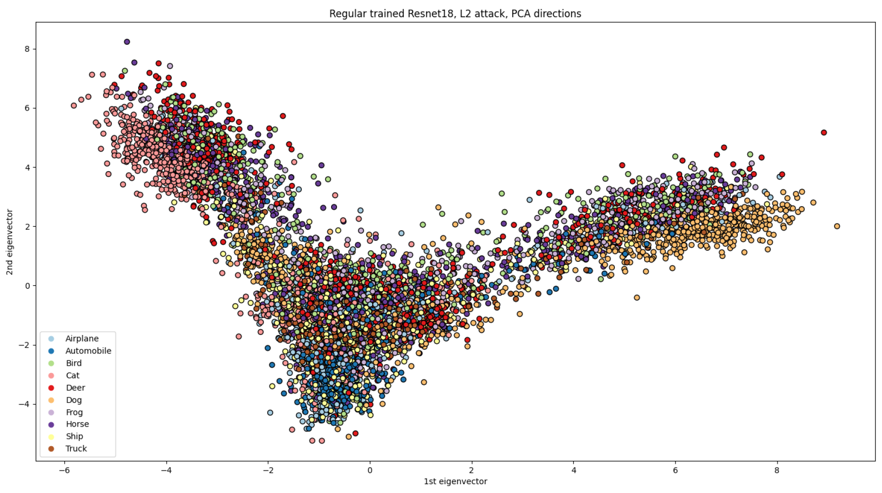
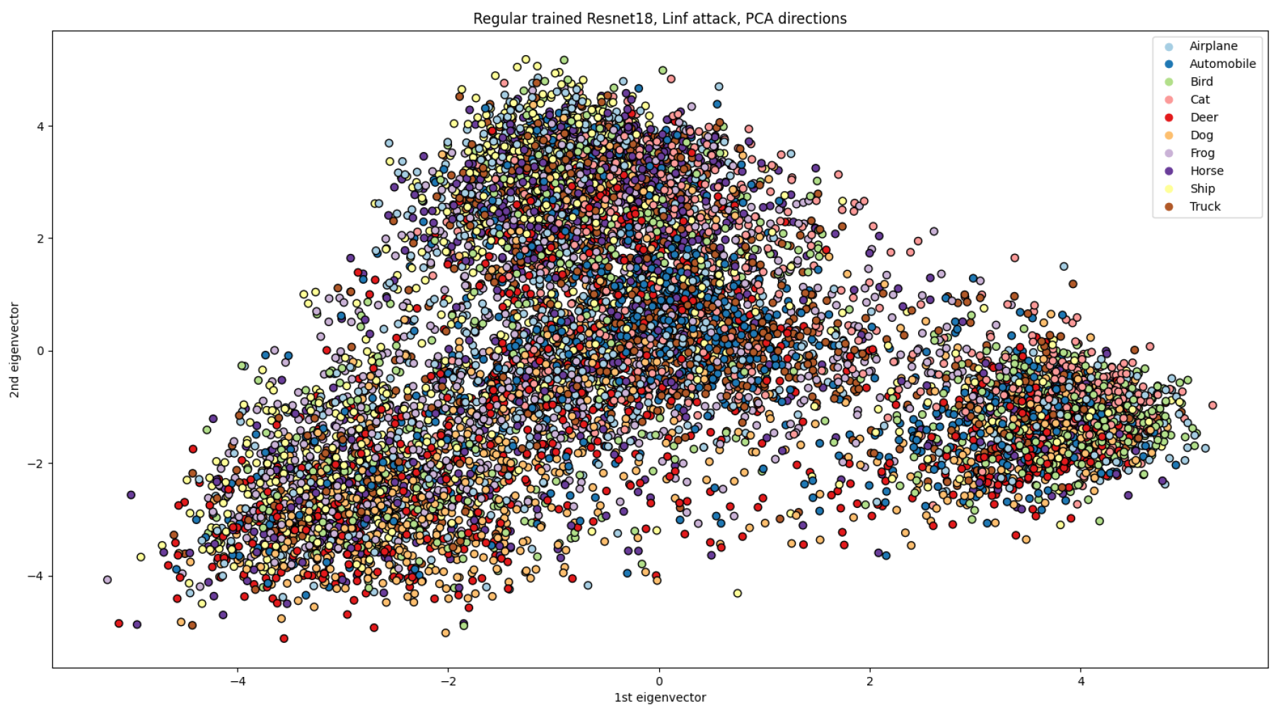
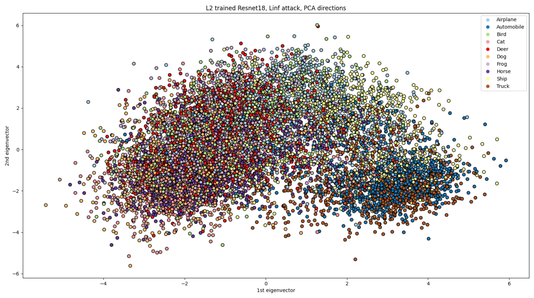
We present the visualisation of representations for different combinations of models and norms of PGD attacks in Figure 4, Figure 5, Figure 6, Figure 7 and Figure 8. Figure 4 depicts the representations of samples from CIFAR-10 for a regularly trained ResNet18, which serves as a baseline case. In Figure 5 and Figure 6, we visualise the data as adversarial samples with $L_2$- and $L_{\infty }$-norms of attack, respectively. Furthermore, we examine the representations of adversarial samples for adversarially trained models in Figure 7 and Figure 8. To challenge the models, we use alter norms of attacks from training ones: the model trained on PGD with an $L_2$-norm is tested on an $L_{\infty }$-norm PGD (Figure 8), and vice versa (Figure 7). We group the representations of different classes by colours in all figures to comprehend how the representations of different classes intermingle under adversarial attacks.

The representations of the regularly trained networks are clustered according to the classes in the data set, as shown in Figure 4. However, when subjected to adversarial attacks, all representations become heavily mixed, resulting in a more challenging classification task due to overlapping representations of different classes. The most mixed representations were observed on the regularly trained network through the $L_{\infty }$-norm PGD attack (Figure 6). On the contrary, adversarial training, as shown in Figure 7 and Figure 8, resulted in some class representations (e.g., “Automobile” or “Truck”) remaining clustered while becoming closer to each other than those without attacks. The same pattern was observed for the $L_2$-norm attack (Figure 6).

5. Impact of Adversarial Training on the Network’s Decision Boundary

As a continuation of generalisation testing, we aim to investigate the impact of robust and adversarial training methods on the decision boundary of a model. Particularly, we show how the mean distance between samples and decision boundaries varies for different models when exposed to adversarial attacks.

We use the idea of Mickisch et al. [10], who utilised the DeepFool attack in Section 2.1.3 to measure this distance. The decision boundary is defined as the set of input images where two or more classes share the same maximum probability, indicating that the classifier is uncertain about the class of the image:

$$\begin{array}{cc}\hfill & D=\{x\in R^n|\exists k_1,k_2=1...c,k_1\ne k_2,\hfill \\ \hfill & f{\left(x\right)}_{k_1}=f{\left(x\right)}_{k_2}=max\left(f\left(x\right)\right)\}\hfill \end{array}$$

(6)

where c is the number of classes. Under this definition, the usage of the DeepFool attack looks natural because it aims to find a perturbation to the closest wrong class. The distance of the sample x to the decision boundary D can be measured as

$$d\left(x\right)=minϵ,s.t.x+ϵ\in D$$

(7)

The pre-trained ResNet50 model is used with 20 steps of PGD attack during training, while ResNet18 models are trained under PGD with only 5 steps. The test data set is CIFAR-10. The outputs of the ResNet18 and ResNet50 models with different training configurations are presented in

Table 8. Mean distance of samples to decision boundary.

Model	Mean ${\mathit{L}}_2$ Distance	Steps
Regularly trained ResNet18	0.1793	1.92
Adversarially trained ResNet18 ($L_2$-norm)	0.659	1.98
Adversarially trained ResNet18 ($L_{\infty }$norm)	0.1018	2.5
Regularly trained ResNet50	0.17	2.58
Adversarially trained ResNet50 ($L_2$-norm)	1.3728	1.77
Adversarially trained ResNet50 ($L_{\infty }$-norm)	1.18	2.66

. The table displays the mean difference between the decision boundaries of models and images from CIFAR-10, calculated using the $L_2$ distance. The “steps” column represents the mean iteration of DeepFool spent during the attack generation. A comparison is made between the models in Table 1, Table 2 and Table 3.

The results indicate that the mean distance for ResNet18-s (for all types of training) from the decision boundary is relatively small, especially for the $L_{\infty }$-norm. A small distance from a sample to the decision boundary implies that it is easier to misclassify this sample because it does not require a significant perturbation. Interestingly, the distance for the $L_{\infty }$-norm adversarially trained model is actually less than training $ϵ$. However, the testing of this model under PGD attack (Table 3) suggests that it has some robustness. Therefore, the reliability of the popular method of model testing used in this study is called into question.

6. Discussion

One explanation for the robustness difference between $L_{\infty }$-norm and $L_2$-norm attacks is according to the adversarial purification framework in Allen-Zhu and Li [28]. In this context, $L_{\infty }$-norm attacks typically manipulate an image by applying the maximum allowable perturbation to each pixel within the defined infinity norm constraint. This kind of attack can exploit the dense mixtures in non-purified features more uniformly across all dimensions of the input space. $L_2$-norm attacks, on the other hand, distribute their perturbations more smoothly and are constrained by the Euclidean distance. This form of attack could be more aligned with the types of perturbations that adversarial training with feature purification is specifically designed to defend against, as the training process aims to stabilize the model against perturbations that have a concentrated energy in the feature space.

7. Conclusions

While strong adversarial attacks on neural networks have already been developed, most of the defense mechanisms still do not guarantee full resistance to them in general. In this study, we consider the impact of adversarial and robust training on a model’s ability to adequately represent adversarial samples. The experiments demonstrate that the model, trained on a “robust” data set, is still vulnerable to some attacks; thus, adversarial attacks do not compromise only non-robust features. Thus, the robust features are not well generalised, especially on the $L_{\infty }$-norm of attack. We assume that the small difference between clean and adversary inputs for the $L_{\infty }$ attack leads to a huge gap in the latent space between them; SVCCA of different attack representations confirms this assumption. Our visualisation of neural network representation also shows the difference between $L_2$- and $L_{\infty }$-norms of attack. Moreover, we discover that $L_{\infty }$-norm adversarial training decreases the distance between the representations and the decision boundary.

In light of these results, we recommend that researchers in the field of adversarial attacks and defense mechanisms pay closer attention to $L_{\infty }$-norm attacks to avoid a false sense of security. It is crucial to consider this norm in their tests to ensure the robustness of models against potential attacks. As the next step in this research, we would like to determine the perturbation coefficient range (experiment in Section 3.2) that should be reasonable for a robust model.

References

- Ilyas, A.; Santurkar, S.; Tsipras, D.; Engstrom, L.; Tran, B.; Madry, A. Adversarial Examples Are Not Bugs, They Are Features. In Proceedings of the Advances in Neural Information Processing Systems 32: Annual Conference on Neural Information Processing Systems 2019, NeurIPS 2019, Vancouver, BC, Canada, 8–14 December 2019; pp. 125–136. [Google Scholar]
- Rasheed, B.; Khan, A.; Kazmi, S.; Hussain, R.; Jalil Piran, M.; Suh, D. Adversarial Attacks on Featureless Deep Learning Malicious URLs Detection. Comput. Mater. Contin. 2021, 680, 921–939. [Google Scholar] [CrossRef]
- Kim, B.; Sagduyu, Y.E.; Davaslioglu, K.; Erpek, T.; Ulukus, S. Channel-Aware Adversarial Attacks Against Deep Learning-Based Wireless Signal Classifiers. IEEE Trans. Wirel. Commun. 2020, 21, 3868–3880. [Google Scholar] [CrossRef]
- Karim, F.; Majumdar, S.; Darabi, H. Adversarial Attacks on Time Series. IEEE Trans. Pattern Anal. Mach. Intell. 2019, 43, 3309–3320. [Google Scholar] [CrossRef]
- Biggio, B.; Corona, I.; Maiorca, D.; Nelson, B.; Šrndić, N.; Laskov, P.; Giacinto, G.; Roli, F. Evasion attacks against machine learning at test time. In Proceedings of the Machine Learning and Knowledge Discovery in Databases: European Conference, ECML PKDD 2013, Prague, Czech Republic, 23–27 September 2013; Proceedings, Part III 13. Springer: Berlin/Heidelberg, Germany, 2013; pp. 387–402. [Google Scholar]
- Chakraborty, A.; Alam, M.; Dey, V.; Chattopadhyay, A.; Mukhopadhyay, D. Adversarial Attacks and Defences: A Survey. arXiv 2018, arXiv:1810.00069. [Google Scholar] [CrossRef]
- Goodfellow, I.J.; Shlens, J.; Szegedy, C. Explaining and Harnessing Adversarial Examples. In Proceedings of the 3rd International Conference on Learning Representations, ICLR 2015, San Diego, CA, USA, 7–9 May 2015. [Google Scholar]
- Madry, A.; Makelov, A.; Schmidt, L.; Tsipras, D.; Vladu, A. Towards Deep Learning Models Resistant to Adversarial Attacks. In Proceedings of the 6th International Conference on Learning Representations, ICLR 2018, Vancouver, BC, Canada, 30 April–3 May 2018. [Google Scholar]
- Moosavi-Dezfooli, S.M.; Fawzi, A.; Frossard, P. DeepFool: A Simple and Accurate Method to Fool Deep Neural Networks. In Proceedings of the 2016 IEEE Conference on Computer Vision and Pattern Recognition (CVPR), Las Vegas, NV, USA, 27–30 June 2016; pp. 2574–2582. [Google Scholar]
- Mickisch, D.; Assion, F.; Greßner, F.; Günther, W.; Motta, M. Understanding the Decision Boundary of Deep Neural Networks: An Empirical Study. arXiv 2020, arXiv:2002.01810. [Google Scholar]
- Wong, E.; Rice, L.; Kolter, J.Z. Fast is better than free: Revisiting adversarial training. In Proceedings of the 8th International Conference on Learning Representations, ICLR 2020, Addis Ababa, Ethiopia, 26–30 April 2020. [Google Scholar]
- Wong, E.; Kolter, Z. Provable defenses against adversarial examples via the convex outer adversarial polytope. In Proceedings of the International Conference on Machine Learning, PMLR, Stockholm, Sweden, 10–15 July 2018; pp. 5286–5295. [Google Scholar]
- Wong, E.; Schmidt, F.R.; Metzen, J.H.; Kolter, J.Z. Scaling provable adversarial defenses. arXiv 2018, arXiv:1805.12514. [Google Scholar]
- Engstrom, L.; Ilyas, A.; Salman, H.; Santurkar, S.; Tsipras, D. Robustness (Python Library). 2019. Available online: https://github.com/MadryLab/robustness (accessed on 13 March 2024).
- Salman, H.; Ilyas, A.; Engstrom, L.; Kapoor, A.; Madry, A. Do adversarially robust imagenet models transfer better? Adv. Neural Inf. Process. Syst. 2020, 33, 3533–3545. [Google Scholar]
- Zhang, C.; Benz, P.; Imtiaz, T.; Kweon, I.S. Understanding adversarial examples from the mutual influence of images and perturbations. In Proceedings of the IEEE/CVF Conference on Computer Vision and Pattern Recognition, Seattle, WA, USA, 14–19 June 2020; pp. 14521–14530. [Google Scholar]
- Engstrom, L.; Gilmer, J.; Goh, G.; Hendrycks, D.; Ilyas, A.; Madry, A.; Nakano, R.; Nakkiran, P.; Santurkar, S.; Tran, B.; et al. A Discussion of ‘Adversarial Examples Are Not Bugs, They Are Features’. Distill 2019, 4. [Google Scholar] [CrossRef]
- Tramèr, F.; Kurakin, A.; Papernot, N.; Goodfellow, I.J.; Boneh, D.; McDaniel, P.D. Ensemble Adversarial Training: Attacks and Defenses. In Proceedings of the 6th International Conference on Learning Representations, ICLR 2018, Vancouver, BC, Canada, 30 April–3 May 2018. [Google Scholar]
- He, K.; Zhang, X.; Ren, S.; Sun, J. Deep residual learning for image recognition. In Proceedings of the IEEE Conference on Computer Vision and Pattern Recognition, Las Vegas, NV, USA, 27–30 June 2016; pp. 770–778. [Google Scholar]
- Krizhevsky, A.; Hinton, G. Learning Multiple Layers of Features from Tiny Images. 2009. Available online: https://www.cs.toronto.edu/~kriz/cifar.html (accessed on 13 March 2024).
- Carlini, N.; Wagner, D.A. Towards Evaluating the Robustness of Neural Networks. In Proceedings of the 2017 IEEE Symposium on Security and Privacy (SP), San Jose, CA, USA, 22–26 May 2017; pp. 39–57. [Google Scholar]
- Szegedy, C.; Vanhoucke, V.; Ioffe, S.; Shlens, J.; Wojna, Z. Rethinking the inception architecture for computer vision. In Proceedings of the IEEE Conference on Computer Vision and Pattern Recognition, Las Vegas, NV, USA, 27–30 June 2016; pp. 2818–2826. [Google Scholar]
- Darlow, L.N.; Crowley, E.J.; Antoniou, A.; Storkey, A.J. Cinic-10 is not imagenet or cifar-10. arXiv 2018, arXiv:1810.03505. [Google Scholar]
- Han, C.; Lei, Y.; Xie, Y.; Zhou, D.; Gong, M. Visual domain adaptation based on modified A-distance and sparse filtering. Pattern Recognit. 2020, 104, 107254. [Google Scholar] [CrossRef]
- Morcos, A.; Raghu, M.; Bengio, S. Insights on representational similarity in neural networks with canonical correlation. Adv. Neural Inf. Process. Syst. 2018, 31, 5727–5736. [Google Scholar]
- An, S.; Bhat, G.; Gumussoy, S.; Ogras, Ü.Y. Transfer Learning for Human Activity Recognition Using Representational Analysis of Neural Networks. ACM Trans. Comput. Healthc. 2020, 4, 1–21. [Google Scholar] [CrossRef]
- Raghu, M.; Gilmer, J.; Yosinski, J.; Sohl-Dickstein, J. Svcca: Singular vector canonical correlation analysis for deep learning dynamics and interpretability. Adv. Neural Inf. Process. Syst. 2017, 30, 6078–6087. [Google Scholar]
- Allen-Zhu, Z.; Li, Y. Feature Purification: How Adversarial Training Performs Robust Deep Learning. In Proceedings of the 2021 IEEE 62nd Annual Symposium on Foundations of Computer Science (FOCS), Denver, CO, USA, 7–10 February 2022; pp. 977–988. [Google Scholar]
Figure 1.
Distributions of samples for adversarially trained ResNet50. Training attack—PGD with -norm, is 0.03.
Figure 2.
Distributions of samples for adversarially trained ResNet50. Training attack—PGD with -norm, is 0.5.
Figure 3.
Distributions of samples for regularly trained ResNet50.
Figure 4.
Representations of regularly trained ResNet18 on clean data set (CIFAR-10).
Figure 5.
Representations of regularly trained ResNet18 on adversarial data set (CIFAR-10), PGD with -norm and 20 steps.
Figure 6.
Figure 7.
Representations of adversarially trained ResNet18 (PGD, -norm) on adversarial data set (CIFAR-10), PGD with -norm and 20 steps.
Figure 8.