Multiplication Symmetric Convolution Property for Discrete Trigonometric Transforms

Kim, Do Nyeon; Rao, K. R.

doi:10.3390/a2031221

Abstract

The symmetric-convolution multiplication (SCM) property of discrete trigonometric transforms (DTTs) based on unitary transform matrices is developed. Then as the reciprocity of this property, the novel multiplication symmetric-convolution (MSC) property of discrete trigonometric transforms, is developed.

Keywords:

symmetric/asymmetric convolution; trigonometric transforms

1. Introduction

Shen et al. [1] developed fast DCT-domain convolution for time/spatial-domain multiplication using DCT type-2. They exploited symmetry and orthogonality for the fast algorithm. Logo-keying operation in the spatial domain can be done in the DCT domain for compressed image/video editing. However, they have not derived the convolution from the symmetric-convolution multiplication (SCM) property of discrete trigonometric transforms (DTTs), which will be the focus of this paper.

Time-domain symmetric convolution for a linear phase filtering application has been developed by Martucci [2] and is called the symmetric-convolution multiplication property of DTTs. Based on the SCM property, Zou et al. [3] have developed a symmetric convolution for linear phase FIR filtering. Filter coefficients consist of symmetric and asymmetric parts.

Based on those earlier works, Reju et al. [4] have finally developed fast circular convolution using DTTs. The input sequences to be convolved need not be symmetric or asymmetric. Thus fast DCTs and DSTs can be used instead of the FFTs for FIR filtering. Generalized fast convolution using numerous transforms as well as the DFT and DTTs has been studied by Korohoda et al. in [5].

In this paper we show that swapping the forward and inverse transforms in the SCM property [2] yields a multiplication-convolution (MSC) property. That is, the convolution of transformed sequences gives the same results as the forward transform after element-by-element multiplication of the data sequences. The necessary scaling factor M for these new properties has been described in the third line below Eq. (20) in [2], saying “it is possible to swap the usage of the forward and inverse transform; in that case, an extra scaling factor may be required”. Here M is the size of the generalized DFT (GDFT) when a DTT is derived from an M-point GDFT. We can get 40 types of MSCs corresponding to 40 types of SCMs in Tables VI, VII of [2].

In (1) of [6], the formulation of the SCM for the unitary matrices is presented, with only the exception of some of the 40 options mentioned by Martucci [2], because they cannot be expressed with the assumed tools. Here, we fill that gap. Consider the following matrix relationship between convolutional/unnormalized DTTs (denoted with lower-case subscript like C_1e) and unitary DTTs (denoted with capital-letter subscript like C_IE).

\begin{matrix} C_{1 e} = \sqrt{2 N} {A_{1}}^{- 1} C_{1 E} A_{1} & C_{2 e} = \sqrt{2 N} {A_{2}}^{- 1} C_{I I E} \end{matrix}

(1)

\begin{matrix} C_{3 e} = \sqrt{2 N} C_{I I I E} A_{2} & C_{4 e} = \sqrt{2 N} C_{I V E} \end{matrix}

(2)

\begin{matrix} S_{1 e} = \sqrt{2 N} S_{I E} & S_{2 e =} \sqrt{2 N} {A_{3}}^{- 1} S_{I I E} \end{matrix}

(3)

\begin{matrix} S_{3 e} = \sqrt{2 N} S_{I I I E} A_{3} & S_{4 e} = \sqrt{2 N} S_{I V E} \end{matrix}

(4)

\begin{matrix} C_{1 o} = \sqrt{2 N - 1} {A_{2}}^{- 1} C_{I O} A_{2} & C_{2 o} = \sqrt{2 N - 1} {A_{2}}^{- 1} C_{I I O} A_{4} \end{matrix}

(5)

\begin{matrix} C_{3 o} = \sqrt{2 N - 1} {A_{4}}^{- 1} C_{I I I O} A_{2} & C_{4 o} = \sqrt{2 N - 1} C_{I V O} \end{matrix}

(6)

\begin{matrix} S_{1 o} = \sqrt{2 N - 1} S_{I O} & S_{2 o} = \sqrt{2 N - 1} S_{I I O} \end{matrix}

(7)

\begin{matrix} S_{3 o} = \sqrt{2 N - 1} S_{I I I O} & S_{4 o} = \sqrt{2 N - 1} {A_{4}}^{- 1} S_{I V O} A_{4} \end{matrix}

(8)

Here the fact that scalars commute with matrices is used for C_3e and others.

\begin{matrix} A_{1} = {[\sqrt{k_{n}}]}_{N + 1} = {[\sqrt{k_{m}}]}_{N + 1} = diag (\frac{1}{\sqrt{2}}, 1, 1, \dots, 1, \frac{1}{\sqrt{2}}), & where m, n = 0, 1, \dots, N \end{matrix}

(9)

\begin{matrix} A_{2} = {[\sqrt{k_{n}}]}_{N} = {[\sqrt{k_{m}}]}_{N} = diag (\frac{1}{\sqrt{2}}, 1, 1, \dots, 1), & where m, n = 0, 1, \dots, N - 1 \end{matrix}

(10)

\begin{matrix} A_{3} = {[\sqrt{k_{n}}]}_{N} = {[\sqrt{k_{m}}]}_{N} = diag (1, 1, \dots, 1, \frac{1}{\sqrt{2}}), & where m, n = 1, 2, \dots, N \end{matrix}

(11)

\begin{matrix} A_{4} = {[\sqrt{l_{n}}]}_{N} = {[\sqrt{l_{m}}]}_{N} = diag (1, 1, \dots, 1, \frac{1}{\sqrt{2}}), & where m, n = 0, 1, \dots, N - 1 \end{matrix}

(12)

\begin{matrix} k_{p} & = 1 / 2 & p = 0, N \\ = 1 & p = 1, 2, \dots, N - 1 \end{matrix}

(13)

\begin{matrix} l_{p} & = 1 & p = 0, 1, \dots, N - 2 \\ = 1 / 2 & p = N - 1 \end{matrix}

(14)

where diag(a₁₁, a₁₁, …, a_NN) implies a diagonal matrix with the diagonal elements as (a₁₁, a₁₁, …, a_NN). I_N is the identity matrix of size N × N.

Let matrices J, K, Q, and R be defined as:

\begin{matrix} J = (\begin{matrix} I_{N} \\ O_{1 \times N} \end{matrix}) & K = (\begin{matrix} O_{1 \times N} \\ I_{N} \end{matrix}) & Q = (\begin{matrix} I_{N - 1} \\ O_{1 \times (N - 1)} \end{matrix}) & R = (\begin{matrix} O_{1 \times (N - 1)} \\ I_{N - 1} \end{matrix}) \\ (N + 1) \times N & (N + 1) \times N & N \times (N - 1) & N \times (N - 1) \end{matrix}

(15)

where O₁_×_N is the zero row-vector, with N elements, whose entries are all zero. Multiplying one of those matrices with an input vector appends a single zero on the top of the first or under the last element of the vector. Multiplying the transpose of one of those matrices with an input vector discards the first or last element of the vector.

2. Symmetric-Convolution Multiplication Property

One of the forty cases of symmetric convolution is proven as an example.

Property.

y = A₁⁻¹C_IE⁻¹ J

ℋ

_C2e C_IIE x [(A8) in Table 3]

Proof.

Equation (A.1) in the appendix of [2] can be rewritten as:

C_{1 e} = 2 {\hat{C}}_{1 e} [k_{n}]_{N + 1}

(16)

where

{\hat{C}}_{1 e}

is the kernel.

C_{I E} = \sqrt{2 / N} [\sqrt{k_{m}}]_{N + 1} {\hat{C}}_{1 e} [\sqrt{k_{n}}]_{N + 1}

(17)

([\sqrt{k_{n}}]_{N + 1})^{- 1} = [\sqrt{1 / k_{n}}]_{N + 1}

(18)

From (16), (17) and (18):

C_{1 e} = [\sqrt{2 N / k_{m}}]_{N + 1} C_{1 E} [\sqrt{k_{n}}]_{N + 1}

(19)

{C_{1 e}}^{- 1} = [\sqrt{1 / k_{n}}]_{N + 1} {C_{I E}}^{- 1} [\sqrt{k_{m} / (2 N)}]_{N + 1}

(20)

From (1) and (10):

{C_{2 e}}^{- 1} = {C_{I I E}}^{- 1} [\sqrt{k_{m} / (2 N)}]_{N}

(21)

Let x and w be input column vectors in time domain. Let y be an output column vector in time domain. Let

ℋ

_C2e be a diagonal matrix defined as

ℋ

_C2e = diag([C_2e w]^T), where superscript T denotes the transpose operator. We rewrite the 8th property in Table VI of [2] as:

\begin{matrix} y & = {C_{1 e}}^{- 1} {ℋ_{C 2 e} C_{2 e} x} \\ = {C_{1 e}}^{- 1} {ℋ_{C 2 e} [\sqrt{2 N / k_{m}}]_{N} C_{I I E} x} \\ = [\sqrt{1 / k_{n}}]_{N + 1} {C_{I E}}^{- 1} [\sqrt{k_{m}}]_{N + 1} J {ℋ_{C 2 e} [\sqrt{1 / k_{m}}]_{N} C_{I I E} x} \end{matrix}

(22)

The matrix J shows up in the last line of (22) for zero padding. Since

ℋ

_C2e and [

\sqrt{1 / k_{m}}

]_N are diagonal matrices, they can commute. Thus:

\begin{matrix} y & = [\sqrt{1 / k_{n}}]_{N + 1} {C_{I E}}^{- 1} J {ℋ_{C 2 e} C_{I I E} x} \\ = [\sqrt{1 / k_{n}}]_{N + 1} {C_{I E}}^{- 1} J {ℋ_{C 2 e} C_{I I E} x} \end{matrix}

(23)

Another example is shown in (11) of [6]. Equation (12) of [6] is expanded to full for our derivation and only results are listed in the first column of Table 3 and Table 4 in the Appendix.

3. Multiplication Symmetric-Convolution Property

Let X and Y be transformed input and output data vectors. Since there are one-to-one correspondences between unitary discrete trigonometric transforms (DTTs), we can exchange the forward transform for inverse one and vice versa as follows. In other words, a pair has the same matrix but has different names. Define h _C3e as:

h _C3e = diag( [(C^3e) ⁻¹ W]^T )

(24)

where C^3e will be defined in (27). That is,

ℋ

_C2e and h _C3e are the same matrix with different names (thus names of DTTs need to change).

Then from (23):

Y = [\sqrt{1 / k_{m}}]_{N + 1} C_{I E} J h_{C 3 e} {C_{I I I E}}^{- 1} X

(25

Notice the forward transform matrix C_IIE is replaced by the inverse transform matrix C_IIIE ⁻¹ since they are the same matrix, and vice versa. Now this equation represents a SCM of DTTs. A key point of this new property is that we need to redefine convolution forms of DCTs and DSTs. The factor of M is divided for the inverse DCT of the convolution form in [2] whereas it is divided for the forward DCT of the new convolution form. M is 2N for even and 2N – 1 for odd. Now new convolution form for DCT 2 is denoted as C^2e:

\begin{matrix} Forward & Inverse \\ (old) & C_{2 e} & \Leftrightarrow & {C_{2 e}}^{- 1} = \frac{1}{M} C_{3 e} \end{matrix}

(26)

\begin{matrix} (new) & C^{2 e} = \frac{1}{M} C_{2 e} & \Leftrightarrow & {(C^{2 e})}^{- 1} = C_{3 e} or {(C^{3 e})}^{- 1} = C_{2 e} \end{matrix}

(27)

The rest of DTTs can be readily obtained from the appendix of [2].

MSC properties can be described in terms of convolutional / unnormalized DTTs to obtain similar results:

\begin{matrix} (11 th SCM in Table IV of [2]) & {C_{3 e}}^{- 1} (C_{3 e} \times C_{3 e}) \end{matrix}

(28)

\begin{matrix} (ours, MSC) & M C^{2 e} ({(C^{2 e})}^{- 1} \times {(C^{2 e})}^{- 1}) \end{matrix}

(29)

Only results are listed. Matrices J, K, Q, and R are required for different index ranges between operands. Link between the index range-based maneuvers described by Martucci [2] and the introduction of the J, K, Q and R matrices is presented in Table 1 and Table 2 for M = 2N and M = 2N − 1, respectively.

4. Applications

For an image resizing (filter) application, one of 40 MSC properties is used. The definition of a normalizing parameter F(k) in [7] needs a minor change as:

\begin{matrix} F (k) = & \sqrt{2} & k = 0 \\ 1 & 1 \leq k \leq N - 1 \end{matrix}

Then we can derive one of MSC properties, which is (4) in [7], from our equation as follows:

\begin{matrix} C_{I I} {x (n) \times w (n)} & = C_{I I} {x (n)} \otimes C^{2 e} {w (n)} \\ = C_{I I} {x (n)} \otimes \frac{1}{2 N} C_{2 e} {w (n)} \end{matrix}

where the symbol ⊗ denotes symmetric convolution. Since C_2e =

\sqrt{2 N}

A₂⁻¹C_IIE in (1),

\begin{matrix} C_{I I} {x (n) \times w (n)} & = C_{I I} {x (n)} \otimes \frac{1}{\sqrt{2 N}} {A_{2}}^{- 1} C_{I I} {w (n)} \end{matrix}

By the associativity of (continuous and discrete) convolution:

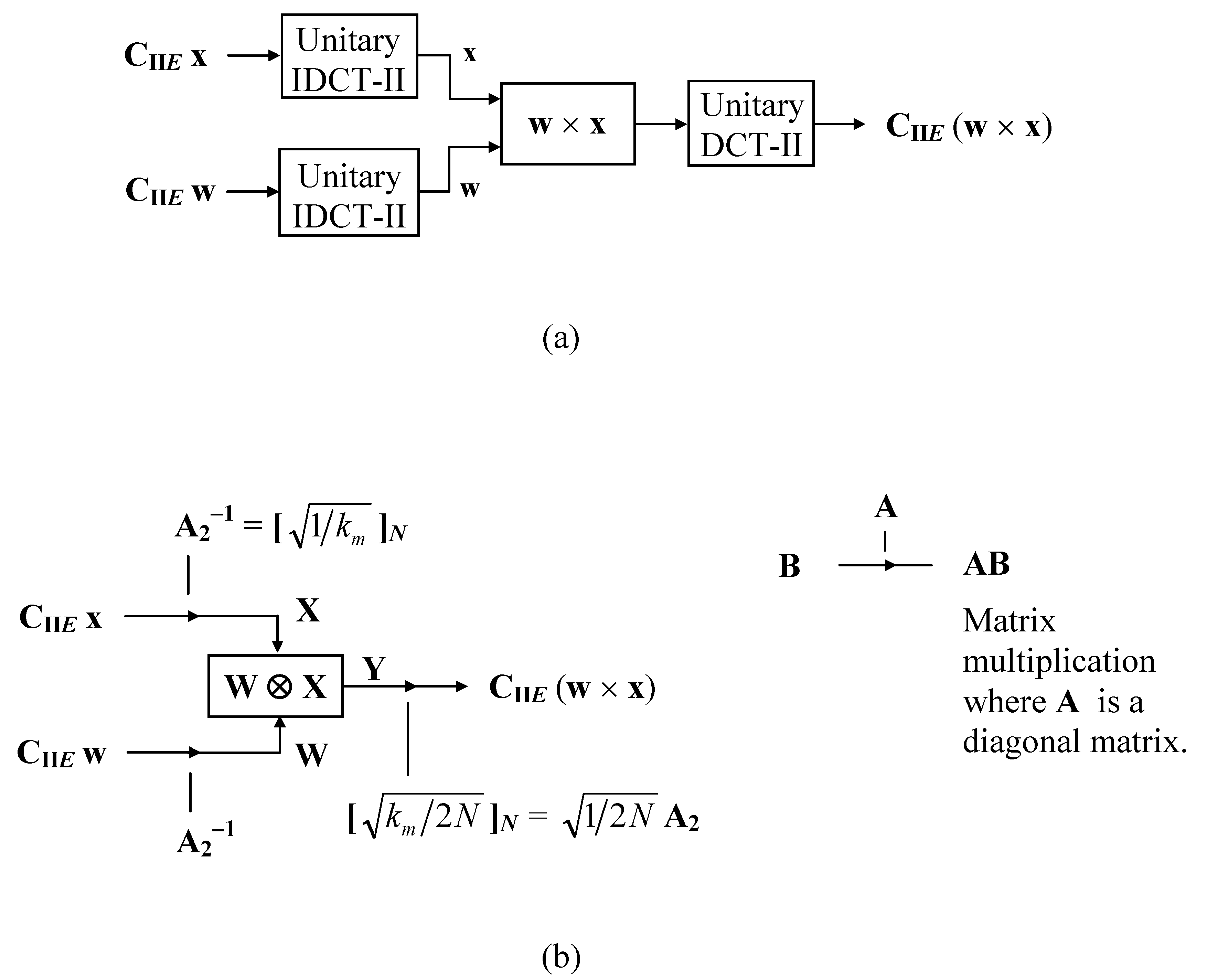
\begin{matrix} C_{I I} {x (n) \times w (n)} & = \frac{1}{\sqrt{2 N}} C_{I I} {x (n)} \otimes {A_{2}}^{- 1} C_{I I} {w (n)} \\ = \frac{1}{\sqrt{2 N}} A_{2} [{A_{2}}^{- 1} C_{I I} {x (n)} \otimes {A_{2}}^{- 1} C_{I I} {w (n)}] \end{matrix}

(30)

This is shown in block diagram format in Fig. 1(b). Since G(k) and F(k) are A₂⁻¹ and

\frac{1}{\sqrt{2 N}}

A₂ in matrix form:

C_II{x(n) × w(n)} = G(k) [ F(k) C_II{x(n)} ⊗ F(k) C_II{w(n)} ]

Convolution has the property of associativity with scalar multiplication. Let F and G be any real sequences. Then:

a(F ⊗ G) = (aF) ⊗ G = F ⊗ (aG)

for any real (or complex) number a.

For a numerical example, let:

w = (1, 2, 3, 4) ^T, x = (1, 0, 3, 2) ^T and N = 4

Then the time domain element-by-element multiplication of the two vectors is:

w × x = (1, 0, 9, 8) ^T

W = A₂⁻¹ C_II w = (a₀, a₁, a₂, a₃) ^T

= (7.071, − 2.230, 0, − 0.159) ^T

X = A₂⁻¹ C_II x
= (4.243, −1.465, 0, 1.689) ^T

Y = W ⊗ X = (W_t + W_h) X
= (36, − 19.823, 0, 11.272) ^T

(31)

where:

W = (W_{t} + W_{h}) (\begin{matrix} a_{0} & a_{1} & a_{2} & a_{3} \\ a_{1} & a_{0} & a_{1} & a_{2} \\ a_{2} & a_{1} & a_{0} & a_{1} \\ a_{3} & a_{2} & a_{1} & a_{0} \end{matrix}) + (\begin{matrix} 0 & a_{1} & a_{2} & a_{3} \\ 0 & a_{2} & a_{3} & 0 \\ 0 & a_{3} & 0 & - a_{3} \\ 0 & 0 & - a_{3} & - a_{2} \end{matrix})

(32)

Equation (32) is

[y_{(N), t}^{3 e}] + [y_{(N), h}^{3 e}]

in [8, p. 2635], and W_t and W_h are a symmetric Toeplitz matrix and a Hankel matrix [9]. Symmetric convolution is represented in matrix multiplication form of (31) using (32). Since the expression inside the square brackets of (30) is the matrix Y defined in (31):

Y = \sqrt{2 N} {A_{2}}^{- 1} C_{I I} (w \times x)

(33)

C_{I I} (w \times x) = \frac{1}{\sqrt{2 N}} A_{2} Y

(34)

Equation (34) corresponds to (30). Thus Y can be computed by using either (33) or (31). In other words, the symmetric convolution of DCT coefficients, Figure 1(b) is an alternative method to computing the DCT of multiplication of two time sequences, Figure 1(a).

Figure 1. For compressed image / video editing, logo-keying operation (alpha blending) can be done in (a) the spatial and (b) transform domains [1]. The symbol × denotes the element-by-element multiplication of the two vectors and ⊗ denotes the symmetric convolution of the two vectors.

5. Conclusions

For logo-keying operation or alpha blending, one image is scaled by α and the other is scaled by (1 − α), where α is a value between zero and one, and then two images are added up. For compressed image / video editing, multiplication operation in logo-keying operation in the spatial can be done in the DTT domain by convolving the unitary DTT coefficients of the two images. For those applications, we have developed 40 types of the MSC properties for the unitary DTTs (DCTs and DSTs [11,12,13]).

Acknowledgements

The authors wish to thank the reviewers.

Appendix

Table 1. Link between the index range-based maneuvers described by Martucci [2] and the introduction of the J, K, Q and R matrices, M = 2N.

**Table 1.** Link between the index range-based maneuvers described by Martucci [2] and the introduction of the J, K, Q and R matrices, M = 2N.
SCM (Symmetric-Conv. Mult.)	Forward transform			$ℋ$			Inverse transform
SCM (Symmetric-Conv. Mult.)	Input index range	Output index range		Input index range	Output index range		Input index range	Output index range
y = S_IE⁻¹ (R^T J^T $ℋ$ _C1e) S_IE x				0→N	1→N−1	R^T J^T
y = S_IE⁻¹ $ℋ$ _S1e R^T J^T C_IE (A₁ x)	0→N	1→N−1	R^T J^T
y = − A₁⁻¹C_IE⁻¹ J R $ℋ$ _S1e S_IE x	1→N−1	0→N	J R
y = C_IIE⁻¹ $ℋ$ _C2e J^T C_IE(A₁ x)	0→N	0→N−1	J^T
y = S_IIE⁻¹ $ℋ$ _S2e K^T C_IE (A₁ x)	0→N	1→N	K^T
y = −C_IIE⁻¹ R $ℋ$ _S1e Q^T S_IIE x	1→N	1→N−1	Q^T				1→N−1	0→N−1	R
y = −C_IIE⁻¹R (Q^T $ℋ$ _S2e) S_IE x				1→N	1→N−1	Q^T	1→N−1	0→N−1	R
y = A₁⁻¹C_IE⁻¹ J $ℋ$ _C2e C_IIE x							0→N−1	0→N	J
y = S_IE⁻¹ (Q^T $ℋ$ _S2e) R^T C_IIE x	0→N−1	1→N−1	R^T	1→N	1→N−1	Q^T
y = S_IE⁻¹ (R^T $ℋ$ _C2e) Q ^T S_IIE x	1→N	1→N−1	Q^T	0→N−1	1→N−1	R^T
y = − A₁⁻¹ C_IE⁻¹ K $ℋ$ _S2e S_IIE x							1→N	0→N	K

Table 2. Link between the index range-based maneuvers described by Martucci [2] and the introduction of the J, K, Q and R matrices, M = 2N − 1.

**Table 2.** Link between the index range-based maneuvers described by Martucci [2] and the introduction of the J, K, Q and R matrices, M = 2N − 1.
SCM (Symmetric-Conv. Mult.)	Forward transform			$ℋ$			Inverse transform
SCM (Symmetric-Conv. Mult.)	Input index range	Output index range		Input index range	Output index range		Input index range	Output index range
y = S_IO⁻¹ (R^T $ℋ$ _C1o) S_IO x				0→N−1	1→N−1	R^T
y = S_IO⁻¹ $ℋ$ _S1o R^T C_IO (A₂ x)	0→N−1	1→N−1	R ^T
y = − A₂⁻¹ C_IO⁻¹ R $ℋ$ _S1o S_IO x							1→N−1	0→N−1	R
y = S_IIO⁻¹ $ℋ$ _S1o R^T C_IIO (A₄ x)	0→N−1	1→N−1	R^T
y = S_IIO⁻¹ (R^T $ℋ$ _C2o) S_IO x				0→N−1	1→N−1	R^T
y = S_IIO⁻¹ (R^T $ℋ$ _C1o) S_IIo x				0→N−1	1→N−1	R^T
y = S_IIO⁻¹ $ℋ$ _S2o R^T C_IO (A₂ x)	0→N−1	1→N−1	R^T
y = − A₄⁻¹ C_IIO⁻¹ R $ℋ$ _S1o S_IIO x							1→N−1	0→N−1	R
y = − A₄⁻¹ C_IIO⁻¹ R $ℋ$ _S2o S_IO x							1→N−1	0→N−1	R
y = S_IO⁻¹ $ℋ$ _S2o R^T C_IIO (A₄ x)	0→N−1	1→N−1	R^T
y = S_IO⁻¹ (R^T $ℋ$ _C2o) S_IIO x				0→N−1	1→N−1	R^T
y = − A₂⁻¹ C_IO⁻¹ R $ℋ$ _S2o S_IIO x							1→N−1	0→N−1	R
y = S_IIIO⁻¹ $ℋ$ _S3o Q^T C_IIIO (A₂ x)	0→N−1	0→N−2	Q ^T
y = S_IIIO⁻¹ Q^T $ℋ$ _C3o Q S_IIIO x	0→N−2	0→N−1	Q				0→N−1	0→N−2	Q^T
y = − A₂⁻¹ C_IIIO⁻¹ Q $ℋ$ _S3o S_IIIO x							0→N−2	0→N−1	Q
y = C_IVO⁻¹ (Q^T $ℋ$ _C3o) C_IVO x				0→N−1	0→N−2	Q ^T
y = C_IVO⁻¹ $ℋ$ _C4o Q^T C_IIIO (A₂ x)	0→N−1	0→N−2	Q ^T
y = A₄⁻¹ S_IVO⁻¹ Q $ℋ$ _S3o C_IVO x							0→N−2	0→N−1	Q
y = A₄⁻¹ S_IVO⁻¹ Q $ℋ$ _C4o S_IIIO x							0→N−2	0→N−1	Q
y = −C_IVO⁻¹ $ℋ$ _S3o Q^T S_IVO (A₄ x)	0→N−1	0→N−2	Q^T
y = −C_IVO⁻¹ (Q^T $ℋ$ _S4o) S_IIIO x				0→N−1	0→N−2	Q^T
y = A₂⁻¹ C_IIIO⁻¹ Q $ℋ$ _C4o C_IVO x							0→N−2	0→N−1	Q
y = S_IIIO⁻¹ (Q^T $ℋ$ _S4o) C_IVO x				0→N−1	0→N−2	Q ^T
y = S_IIIO⁻¹ $ℋ$ _C4o Q^T S_IVO (A₄ x)	0→N−1	0→N−2	Q^T

Table 3. 20 of 40 types of SCM and MSC properties for the DTTs, M = 2N.

**Table 3.** 20 of 40 types of SCM and MSC properties for the DTTs, M = 2N.
SCM (Symmetric-Conv. Mult.)	MSC (Mult. Symmetric-Conv.)
y = A₁⁻¹C_IE⁻¹ $ℋ$ _C1e C_IE (A₁ x)	Y = A₁⁻¹C_IE h_C1e C_IE ⁻¹(A₁ X)	(A1)
y = S_IE⁻¹ (R^T J^T $ℋ$ _C1e) S_IE x	Y = S_IE (R^T J^T $ℋ$ _C1e) S_IE⁻¹ X	(A2)
y = S_IE⁻¹ $ℋ$ _S1e R^T J^T C_IE (A₁ x)	Y = S_IE $ℋ$ _S1e R^T J^T C_IE⁻¹ (A₁ X)
y = − A₁⁻¹C_IE⁻¹ J R $ℋ$ _S1e S_IE x	Y = − A₁⁻¹C_IE J Rh_S1e S_IE ⁻¹ X	(A3)
y = C_IIE⁻¹ $ℋ$ _C1e C_IIE x	Y = C_IIIE h_C1e C_IIIE ⁻¹ X	(A4)
y = C_IIE ⁻¹ $ℋ$ _C2e J^T C_IE(A₁ x)	Y = C_IIIE h_C3e J^T C_IE⁻¹(A₁ X)
y = S_IIE⁻¹ $ℋ$ _S1e C_IIE x	Y = S_IIIE h_S1e C_IIIE⁻¹ X	(A5)
y = S_IIE⁻¹ $ℋ$ _C2e S_IE x	Y = S_IIIE h_C3e S_IE⁻¹ X
y = S_IIE⁻¹ $ℋ$ _C1e S_IIE x	Y = S_IIIE h_C1e S_IIIE⁻¹ X	(A6)
y = S_IIE⁻¹ $ℋ$ _S2e K^T C_IE (A₁ x)	Y = S_IIE h_S3e K^T C_IE⁻¹(A₁ X)
y = −C_IIE⁻¹ R $ℋ$ _S1e Q^T S_IIE x	Y = −C_IIIE R h_S1e Q^T S_IIIE⁻¹ X	(A7)
y = −C_IIE⁻¹R (Q^T $ℋ$ _S2e) S_IE x	Y = −C_IIIE R (Q^T h_S3e) S_IE⁻¹ X
y = A₁⁻¹C_IE⁻¹ J $ℋ$ _C2e C_IIE x	Y = A₁⁻¹C_IE J h _C3e C_IIIE ⁻¹ X	(A8)
y = S_IE⁻¹ (Q^T $ℋ$ _S2e) R^T C_IIE x	Y = S_IE (Q^T h _S3e) R^T C_IIIE⁻¹ X	(A9)
y = S_IE⁻¹ (R^T $ℋ$ _C2e) Q ^T S_IIE x	Y = S_IE (R^T h_C3e) Q ^T S_IIIE⁻¹ X
y = − A₁⁻¹ C_IE⁻¹ K $ℋ$ _S2e S_IIE x	Y = − A₁⁻¹ C_IE K h _S3e S_IIIE ⁻¹ X	(A10)
y = A₂⁻¹ C_IIIE⁻¹ $ℋ$ _C3e C_IIIE(A₂ x)	Y = A₂⁻¹ C_IIE h _C2e C_IIE⁻¹(A₂ X)	(A11)
y = A₃⁻¹ S_IIIE⁻¹ $ℋ$ _S3e C_IIIE(A₂ x)	Y = A₃⁻¹ S_IIE h _S2e C_IIE ⁻¹(A₂ X)	(A12)
y = A₃⁻¹ S_IIIE⁻¹ $ℋ$ _C3e S_IIIE(A₃ x)	Y = A₃⁻¹ S_IIE h _S2e S_IIE ⁻¹(A₃ X)
y = A₂⁻¹ C_IIIE⁻¹ $ℋ$ _S3e S_IIIE(A₃ x)	Y = A₂⁻¹ C_IIE h _S2e S_IIE ⁻¹(A₃ X)	(A13)
y = C_IVE⁻¹ $ℋ$ _C3e C_IVE x	Y = C_IVE h _C2e C_IVE⁻¹ X
y = C_IVE⁻¹ $ℋ$ _C4e C_IIIE(A₂ x)	Y = C_IVE h _C4e C_IIE⁻¹(A₂ X)	(A14)
y = S_IVE⁻¹ $ℋ$ _S3e C_IVE x	Y = S_IVEh _S2e C_IVE⁻¹X	(A15)
y = S_IVE⁻¹ $ℋ$ _C4e S_IIIE(A₃ x)	Y = S_IVEh _C4e S_IIE⁻¹(A₃ X)
y = S_IVE⁻¹ $ℋ$ _C3e S_IVE x	Y = S_IVE h _C2e S_IVE⁻¹ X	(A16)
y = S_IVE⁻¹ $ℋ$ _S4e C_IIIE(A₂ x)	Y = S_IVE h _S4e C_IIE⁻¹(A₂ X)
y = −C_IVE⁻¹ $ℋ$ _S3e S_IVE x	Y = −C_IVE h _S2e S_IVE⁻¹ X	(A17)
y = −C_IVE⁻¹ $ℋ$ _S4e S_IIIE(A₃ x)	Y = −C_IVE h _S4e S_IIE⁻¹ (A₃ X)
y = A₂⁻¹ C_IIIE⁻¹ $ℋ$ _C4e C_IVE x	Y = A₂⁻¹ C_IIE h $ℋ$ _C4e C_IVE ⁻¹ X	(A18)
y = A₃⁻¹ S_IIIE⁻¹ $ℋ$ _S4e C_IVE x	Y = A₃⁻¹ S_IIE h _S4e C_IVE⁻¹ X	(A19)
y = A₃⁻¹ S_IIIE⁻¹ $ℋ$ _C4e S_IVE x	Y = A₃⁻¹ S_IIE h _C4e S_IVE⁻¹ X
y = − A₂⁻¹ C_IIIE⁻¹ $ℋ$ _S4e S_IVE x	Y = − A₂⁻¹ C_IIE h _S4e S_IVE⁻¹ X	(A20)

Table 4. 20 of 40 types of SCM and MSC properties for the DTTs, M = 2N − 1.

**Table 4.** 20 of 40 types of SCM and MSC properties for the DTTs, M = 2N − 1.
SCM (Symmetric-Conv. Mult.)	MSC (Mult. Symmetric-Conv.)
y = A₂⁻¹ C_IO⁻¹ $ℋ$ _C1o C_IO (A₂ x)	Y = A₂⁻¹ C_IO h _C1o C_IO ⁻¹(A₂ X)	(A21)
y = S_IO⁻¹ (R^T $ℋ$ _C1o) S_IO x	Y = S_IO (R^T h _C1o) S_IO⁻¹ X	(A22)
y = S_IO⁻¹ $ℋ$ _S1o R^T C_IO (A₂ x)	Y = S_IO h _S1o R^T C_IO⁻¹(A₂ X)
y = − A₂⁻¹ C_IO⁻¹ R $ℋ$ _S1o S_IO x	Y = − A₂⁻¹ C_IO R h _S1o S_IO ⁻¹ X	(A23)
y = A₄⁻¹ C_IIO⁻¹ $ℋ$ _C1o C_IIO (A₄ x)	Y = A₄⁻¹ C_IIIO h _C1o C_IIIO ⁻¹ (A₄ X)	(A24)
y = A₄⁻¹ C_IIO⁻¹ $ℋ$ _C2o C_IO (A₂ x)	Y = A₄⁻¹ C_IIIO h _C3o C_IO⁻¹(A₂ X)
y = S_IIO⁻¹ $ℋ$ _S1o R^T C_IIO (A₄ x)	Y = S_IIIO h _S1o R^T C_IIIO ⁻¹ (A₄ X)	(A25)
y = S_IIO⁻¹ (R^T $ℋ$ _C2o) S_IO x	Y = S_IIIO (R ^T h _C3o) S_IO⁻¹ X
y = S_IIO⁻¹ (R^T $ℋ$ _C1o) S_IIo x	Y = S_IIIO (R^T h _C1o) S_IIIO⁻¹ X	(A26)
y = S_IIO⁻¹ $ℋ$ _S2o R^T C_IO (A₂ x)	Y = S_IIIO h _S3o R^T C_IO⁻¹ (A₂ X)
y = − A₄⁻¹ C_IIO⁻¹ R $ℋ$ _S1o S_IIO x	Y = − A₄⁻¹ C_IIIO R h _S3o S_IO⁻¹ X	(A27)
y = − A₄⁻¹ C_IIO⁻¹ R $ℋ$ _S2o S_IO x	Y = − A₄⁻¹ C_IIIO R h _S1o S_IIIO⁻¹ X
y = A₂⁻¹ C_IO⁻¹ $ℋ$ _C2o C_IIO (A₄ x)	Y = A₂⁻¹ C_IOh _C3o C_IIIO⁻¹ (A₄ X)	(A28)
y = S_IO⁻¹ $ℋ$ _S2o R^T C_IIO (A₄ x)	Y = S_IO h _S3o R^T C_IIIO⁻¹ (A₄ X)	(A29)
y = S_IO⁻¹ (R^T $ℋ$ _C2o) S_IIO x	Y = S_IO⁻¹ (R^T h _C3o) S_IIIO X
y = − A₂⁻¹ C_IO⁻¹ R $ℋ$ _S2o S_IIO x	Y = − A₂⁻¹ C_IO R h _S3o S_IIIO⁻¹ X	(A30)
y = A₂⁻¹ C_IIIO⁻¹ $ℋ$ _C3o C_IIIO(A₂ x)	Y = A₂⁻¹ C_IIO h _C2o C_IIO⁻¹(A₂ X)	(A31)
y = S_IIIO⁻¹ $ℋ$ _S3o Q^T C_IIIO (A₂ x)	Y = S_IIO h _S2o Q^T C_IIO⁻¹(A₂ X)	(A32)
y = S_IIIO⁻¹ Q^T $ℋ$ _C3o Q S_IIIO x	Y = S_IIO Q^T h _S2o Q S_IIO⁻¹ X
y = − A₂⁻¹ C_IIIO⁻¹ Q $ℋ$ _S3o S_IIIO x	Y = − A₂⁻¹ C_IIO Q h _S2o S_IIO⁻¹ X	(A33)
y = C_IVO⁻¹ (Q^T $ℋ$ _C3o) C_IVO x	Y = C_IVO (Q^T h _C2o) C_IVO⁻¹ X	(A34)
y = C_IVO⁻¹ $ℋ$ _C4o Q^T C_IIIO (A₂ x)	Y = C_IVO h _C4o Q^T C_IIO⁻¹(A₂ X)
y = A₄⁻¹ S_IVO⁻¹ Q $ℋ$ _S3o C_IVO x	Y = A₄⁻¹ S_IVO Q h _S2o C_IVO⁻¹ X	(A35)
y = A₄⁻¹ S_IVO⁻¹ Q $ℋ$ _C4o S_IIIO x	Y = A₄⁻¹ S_IVOQ h _C4o S_IIO⁻¹ X
y = A₄⁻¹ S_IVO⁻¹ $ℋ$ _C3o S_IVO (A₄ x)	Y = A₄⁻¹ S_IVO h _C2o S_IVO⁻¹ (A₄ X)	(A36)
y = A₄⁻¹ S_IVOE⁻¹ $ℋ$ _S4o C_IIIO (A₂ x)	Y = A₄⁻¹ S_IVOh _S4o C_IIO⁻¹ (A₂ X)
y = − C_IVO⁻¹ $ℋ$ _S3o Q^T S_IVO (A₄ x)	Y = − C_IVOh _S2o Q^T S_IVO⁻¹ (A₄ X)	(A37)
y = − C_IVO⁻¹ (Q^T $ℋ$ _S4o) S_IIIO x	Y = − C_IVO (Q^T h _S4o) S_IIIO⁻¹ X
y = A₂⁻¹ C_IIIO⁻¹ Q $ℋ$ _C4o C_IVO x	Y = A₂⁻¹ C_IIO Q h _C4o C_IVO⁻¹ X	(A38)
y = S_IIIO⁻¹ (Q^T $ℋ$ _S4o) C_IVO x	Y = S_IIO (Q^T h _S4o) C_IVO⁻¹ x	(A39)
y = S_IIIO⁻¹ $ℋ$ _C4o Q^T S_IVO (A₄ x)	Y = S_IIO⁻¹ h _C4o Q^T S_IVO⁻¹ (A₄ X)
y = − A₂⁻¹ C_IIIO⁻¹ $ℋ$ _S4o S_IVO (A₄ x)	Y = − A₂⁻¹ C_IIO h _S4o S_IVO⁻¹ (A₄ x)	(A40)

References and Notes

Shen, Bo; Sethi, I.K.; Bhaskaran, V. DCT convolution and its application in compressed domain. IEEE T. Circ. Syst. Vid. 1998, 8, 947–952. [Google Scholar]
Martucci, S.A. Symmetric convolution and the discrete sine and cosine transforms. IEEE Trans. SP 1994, 42, 1038–1051. [Google Scholar] [CrossRef]
Zou, X.; Muramatsu, S.; Kiya, H. The generalized overlap-add and overlap-save methods using discrete sine and cosine transforms for FIR filtering. In Proceedings of the 3rd IEEE Int’l Conf. on Signal Processing, ICSP'96, Beijing, China, October 1996; pp. 91–94.
Reju, V.G.; Koh, S.N.; Soon, I.Y. Convolution using discrete sine and cosine transforms. IEEE Signal Proc. Let. 2007, 14, 445–448. [Google Scholar] [CrossRef]
Korohoda, P.; Dabrowski, A. Generalized convolution as a tool for the multi-dimensional filtering tasks. Multidim. Syst. Sign. P. 2008, 19, 361–377. [Google Scholar] [CrossRef]
Foltz, T.M.; Welsh, B.M.; Holmberg, C.D. Symmetric convolution using unitary transform matrices. IEEE T. Signal Proces. 2000, 48, 2691–2692. [Google Scholar] [CrossRef]
Park, Y.S.; Park, H.W. Design and analysis of an image resizing filter in the block-DCT domain. IEEE T. Circ. Syst. Vid. 2004, 14, 274–279. [Google Scholar]
Sánchez, V.; García, P.; Peinado, A.M.; Segura, J.C.; Rubio, A.J. Diagonalizing properties of the discrete cosine transforms. IEEE T. Signal Proces. 1995, 43, 2631–2641. [Google Scholar] [CrossRef]
Sánchez, V.; García, P.; Peinado, A.M.; Segura, J.C.; Rubio, A.J. Generating matrices for the discrete sine transforms. IEEE T. Signal Proces. 1996, 44, 2644–2646. [Google Scholar] [CrossRef]
Martucci, S.A. Image resizing in the discrete sine and cosine domain. In Proceedings of the IEEE International Conference on Image Processing 1995, Washington, DC, USA, October 1995; Volume 2, pp. 244–247.
Foltz, T.M.; Welsh, B.M. Symmetric convolution of asymmetric multidimensional sequences using discrete trigonometric transforms. IEEE T. Image Proces. 1999, 8, 640–651. [Google Scholar] [CrossRef] [PubMed]
Rao, K.R.; Yip, P. Discrete Cosine Transform: Algorithms, Advantages, And Applications; Academic Press: London, England, 1990. [Google Scholar]
Britanak, V.; Yip, P.; Rao, K.R. Discrete Cosine and Sine Transforms; Academic Press (Elsevier): Orlando, FL, USA, 2007; pp. 32–38. [Google Scholar]

© 2009 by the authors; licensee Molecular Diversity Preservation International, Basel, Switzerland. This article is an open-access article distributed under the terms and conditions of the Creative Commons Attribution license (http://creativecommons.org/licenses/by/4.0/).

Article Metrics

Citations

Article Access Statistics

Journal Statistics

Multiple requests from the same IP address are counted as one view.