A 3/2-Approximation Algorithm for the Graph Balancing Problem with Two Weights

Abstract

In the pursuit of finding subclasses of the makespan minimization problem on unrelated parallel machines that have approximation algorithms with approximation ratio better than 2, the graph balancing problem has been of current interest. In the graph balancing problem each job can be non-preemptively scheduled on one of at most two machines with the same processing time on either machine. Recently, Ebenlendr, Krčál, and Sgall (Algorithmica 2014, 68, 62–80.) presented a $7/4$-approximation algorithm for the graph balancing problem. Let $r,s\in {\mathbb{Z}}^{+}$. In this paper we consider the graph balancing problem with two weights, where a job either takes r time units or s time units. We present a $3/2$-approximation algorithm for this problem. This is an improvement over the previously best-known approximation algorithm for the problem with approximation ratio 1.652 and it matches the best known inapproximability bound for it.

1. Introduction

Let $G=(V,E,\mathbf{p},\mathbf{q})$ be a weighted multigraph, where V is the set of vertices, E is the set of edges, $\mathbf{p}=(p_1,\dots ,p_{\left|E\right|})$ are non-negative edge weights, and $\mathbf{q}=(q_1,\dots ,q_{\left|V\right|})$ are the dedicated loads. A dedicated load $q_v$ of vertex v is the sum of the weights of self-loops incident on v in the multigraph; we assume the self-loops are removed from G. An orientation $\gamma :E\to V$ orients each edge $e\in E$ towards one of its endpoints. Given a weighted multigraph G, the graph balancing problem is to find an orientation γ where the maximum load of the vertices is minimized, where the load of a vertex v is defined as $q_v+{\sum }_{e|\gamma (e)=v}{p}_e$.

Let $r,s\in {\mathbb{Z}}^{+}$, where $r<s$. We focus on a special case of this problem we call the graph balancing problem with two weights (GBP2W), where the edges have either weight r or s and each dedicated load is of the form $ar+bs$ for $a,b\in {\mathbb{Z}}^{+}\cup \left\{0\right\}$.

The graph balancing problem is a special case of the makespan minimization problem on unrelated parallel machines ($R\left|\right|C_{max}$ in Graham notation, see [1]). Presently, the best-known approximation algorithms for $R\left|\right|C_{max}$ have approximation ratio 2. The first 2-approximation algorithm for $R\left|\right|C_{max}$ was presented by Lenstra et al. [2], and in 2005 a $(2-1/m)$-approximation algorithm was given by Shchepin and Vakhania [3], where m is the number of machines. These 2-approximation algorithms utilize linear programming, but it is worth noting that there is a combinatorial 2-approximation algorithm by Gairing et al. [4] that employs generalized flow networks. Finding an approximation algorithm with approximation ratio better than 2 for $R\left|\right|C_{max}$ is an important open problem in scheduling theory, and trying to get any further insight into the problem through the study of subclasses of $R\left|\right|C_{max}$ has been of attention lately [5,6,7,8,9,10,11,12,13].

Recently, Ebenlendr et al. [7] gave a $7/4$-approximation algorithm for the graph balancing problem. In addition, Ebenlendr et al. [14] showed that for $p<3/2$, there is no p-approximation algorithm for the graph balancing problem when the edges of the multigraph have weight $1/2$ or 1, unless P=NP. Note that this hardness result was also independently proven by Asahiro et al. [5,15]. This matches the inapproximability bound for the makespan minimization problem on unrelated parallel machines given by Lenstra et al. [2], so, GBP2W is worth investigating due to being one of the simplest scheduling problems presently known to share inapproximability properties with $R\left|\right|C_{max}$.

$3/2$-approximation algorithms have been presented for some special cases of GBP2W. The graph orientation problem with two weights is a NP-hard special case of GBP2W where G is simple, and every dedicated load $q_v=0$. In [5,15], Asahiro et al. gave two approximation algorithms that achieve the bound $3/2$ for variants of the graph orientation problem with two weights: one called Cycle-Canceling when $r=1$ and $s=2$; and another called Refined Cycle-Canceling when $r=1$ and $s=3$. Later, Kolliopoulos and Moysoglou [9] gave a $3/2$-approximation algorithm for GBP2W when $r=1$ and $s=k$, where k is a positive integer (Theorem 4.1).

Most recently, Kolliopoulos and Moysoglou [9] presented a 1.652-approximation algorithm for GBP2W. Their approximation algorithm employs binary search, and for a given estimation of the optimal load T different approximation algorithms are used based on the values of the weights with respect to T. A core component of this approximation algorithm is a flow-network based approximation algorithm for the two-valued case of the restricted assignment problem introduced in the same paper. In this paper we present a $3/2$-approximation algorithm for GBP2W. We adopt a technique of considering particular intervals for the weights during a binary search similar to that of by Kolliopoulos and Moysoglou to derive our $3/2$-approximation algorithm.

To conclude this section, we outline the remainder of this paper. In Section 2, we present our contribution—a $3/2$-approximation algorithm for GBP2W. After describing our algorithm, we give subroutines used by the algorithm and their correctness in Section 2.1, Section 2.2, Section 2.3 and Section 2.4, then prove our algorithm is indeed a $3/2$-approximation algorithm for GBP2W in Section 2.5. In Section 3, we conclude our paper.

2. Algorithm

Similar to the algorithm by Lenstra et al. [2], our approximation algorithm uses an estimation T of the maximum load of a vertex in an optimal orientation as a parameter. The algorithm GB2W presented below as Algorithm 1 finds a solution of value at most $3T/2$ if a solution of value at most T exists. We combine this algorithm with a binary search procedure to find the smallest value for T for which an orientation with load at most $3T/2$ for the graph balancing problem with two weights is found: if for a given T the algorithm does not find a solution of value at most $3T/2$ then the value of T is increased in the binary search; otherwise it is decreased. By the above property of our algorithm this smallest value of T must be less than or equal to the value of an optimum solution, hence our algorithm has approximation ratio $3/2$.

The remainder of this section gives Lemmas 1–4 which provide the subroutines used by our algorithm, then in Theorem 5 we prove our algorithm is a $3/2$-approximation algorithm for GBP2W. First, we present Lemma 1 which covers Step 4 of our algorithm. Note that in Step 1 the algorithm scales the weights so the estimation for the optimum load is $T=1$. We define a big edge e to be an edge with weight $p_e>1/2$; otherwise, we call an edge small. Let the value for an optimum solution for the problem be denoted as $OPT$. From this point forward, we assume that as edges are oriented in Steps 4–5.3, they are removed from G.

Algorithm 1: GB2W $(G=(V,E,\mathbf{p},\mathbf{q}),T)$

Input:  Multigraph G, value T. Output:  An orientation γ for the edges in E with maximum vertex load at most $3T/2$ or FAIL. If FAIL is returned there is no orientation for E with maximum vertex load T. Divide edge weights and vertex dedicated loads by T; set $T=1$. If $s>1$ or $q_v>1$ for any $v\in V$ then return FAIL. If $r,s\in (0,1/2]$ then apply the algorithm by Lenstra et al. [2]. If $r,s\in (1/2,1]$ then apply the algorithm given in Lemma 1. If $r\in (0,1/2]$ and $s\in (1/2,1]$ we consider three subcases. Let $k=\lfloor 1/r\rfloor$, so $1/(k+1)<r\le 1/k$. 5.1. If $k/(k+1)\le s\le 1$ then apply the algorithm in Lemma 2. 5.2. If $(k-1)/k\le s<k/(k+1)$ then apply the algorithm in Lemma 3. 5.3. If $1/2<s<(k-1)/k$ then apply the algorithm in Lemma 4. If any of the algorithms used in Steps 3–5 reports FAIL or if the solution computed by them has value larger than $3/2$ then return FAIL; otherwise return the solution computed in the above steps.

2.1. Step 4

Lemma 1. 

There is a polynomial-time algorithm for the graph balancing problem with two rational weights $r,s\in (1/2,1]$ that either finds a solution of value at most 1 or proves that $OPT>1$.

Proof. 

Since $r,s\in (1/2,1]$, each edge of G is a big edge. If there is an orientation for the edges with maximal load at most 1, then at most one edge can be oriented towards a given vertex. Therefore, if any connected component $C=(V_C,E_C)$ of G has $|E_C|>|V_C|$ then there is no solution for the graph balancing problem of value at most 1. The algorithm is as follows (Big_$rs$, Algorithm 2).

Algorithm 2: Big_$rs (G=(V,E,\mathbf{p},\mathbf{q}))$

Input:  Multigraph G. Output:  An orientation γ for the edges in E with maximum vertex load at most 1 or FAIL. If FAIL is returned there is no orientation for E with maximum vertex load 1. If any connected component $C=(V_C,E_C)$ of G has $|E_C|>|V_C|$, then return FAIL. While G has cycles do 2.1. Find a cycle $C^{\prime }$ of G. 2.2. Mark the vertices in $C^{\prime }$ and orient the cycle in an arbitrary direction. Remove the edges in $C^{\prime }$ from G. For every maximal tree T in G do 3.1. If there is a vertex v in T with $q_v>0$ or that is marked, then set v as the root of T 3.2. else choose any vertex v in T as the root. 3.3. Orient all the edges in T away from its root. 3.4. If any edge in T is oriented towards a vertex u with $q_u>0$ or that is marked then return FAIL. Return orientation for the edges of G.

Multigraph G must have at most $\left|V\right|$ edges, and an optimal orientation matches each edge to a unique vertex with no dedicated load. If a solution of value at most 1 exists, it must be found in Steps 2 and 3. The above algorithm runs in $O(|V|+|E|)$ time.  ☐

2.2. Step 5.1

Next, we consider the case handled in Step 5.1 of the algorithm, namely when $k/(k+1)\le s\le 1$ and $k=\lfloor 1/r\rfloor$ so $1/(k+1)<r\le 1/k$. In Lemma 2, we utilize the property that $r+s>1$, which means that if $OPT\le 1$, then no small edge can be oriented with a big edge towards a given vertex without causing the maximal load to be greater than 1.

Lemma 2. 

For any $k\ge 2$, there is a polynomial-time algorithm for the graph balancing problem with two rational weights $r,s$, where $1/(k+1)<r\le 1/k$ and $k/(k+1)\le s\le 1$ that either finds a solution of value at most $3/2$ or proves that $OPT>1$.

Proof. 

If $OPT\le 1$, since $r+s>1$, for any optimal orientation either at most a big edge is oriented towards a vertex, or at most k small edges are oriented towards a vertex. This property is natural to encode into a flow network. To find an orientation for the edges of the weighted multigraph $G=(V,E,\mathbf{p},\mathbf{q})$, we use a multi-level flow network similar to that in [9].

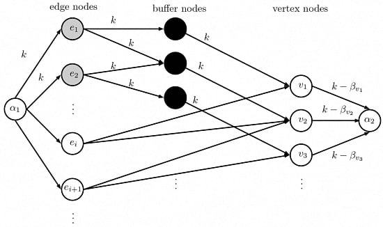
We build a flow network N as follows. First, we consider the dedicated loads of the vertices. For each vertex $v\in V$, define a value ${\beta }_v\ge 0$ as follows: if $q_v\ge s$, set ${\beta }_v=k$; otherwise there is a non-negative integer $p_v$ so that $q_v=p_{v}r$, assign ${\beta }_v=p_v$. The flow network will have a source ${\alpha }_1$ and sink ${\alpha }_2$. We will describe the network level by level. First, we have a level of nodes in the network called edge nodes. These are nodes corresponding to the edges in the multigraph. There are two types of edge nodes: big edge nodes for edges with weight s; and small edge nodes for those with weight r. From source ${\alpha }_1$, add an arc from ${\alpha }_1$ to each edge node, and set its capacity to k if it is to a big edge node, and 1 otherwise. The next level consists of buffer nodes, one for each vertex. The buffer nodes are added to prevent excess flow from being contributed by the big edge nodes. While this part of the network is not important for proving this lemma, it will be vital for how we later use this network in Lemma 3. For each big edge $\{u,v\}\in E$, add arcs with capacity k from its big edge node to buffer nodes u and v. For the next level of the network, create a vertex node that will correspond to each vertex in the multigraph. For each buffer node for $v\in V$, add an arc from its buffer node to its vertex node with capacity k. Next, for each small edge $\{u,v\}\in E$, include arcs with capacity 1 from its small edge node to vertex nodes u and v. Finally, for each vertex $v\in V$, add an arc from vertex node v to sink ${\alpha }_2$ with capacity $k-{\beta }_v$. The resulting flow network is shown in Figure 1.

Before we proceed to describe the algorithm, we show that this network has the following property: if $OPT\le 1$, an integral maximum flow on this network saturates all the arcs leaving source ${\alpha }_1$. Consider any optimal orientation ${\gamma }^{*}$. Using ${\gamma }^{*}$ we construct a flow function in which every small edge node receives 1 unit of flow, and each big edge node receives k units of flow from the source ${\alpha }_1$. For each big edge $\{u_1,u_2\}$ of G with ${\gamma }^{*}(u_1,u_2)=u_i$, if u is the big edge node for $\{u_1,u_2\}$ send k units of flow from ${\alpha }_1$ to u, k units of flow from u to buffer node $u_i$, k units of flow from buffer node $u_i$ to vertex node $u_i$, and k units of flow from $u_i$ to the sink ${\alpha }_2$. Similarly, for each edge $\{u_1,u_2\}$ represented by small edge node u and ${\gamma }^{*}(u_1,u_2)=u_i$, send 1 unit of flow from ${\alpha }_1$ to u, from u to vertex node $u_i$, and from $u_i$ to ${\alpha }_2$. It is not hard to see that this flow function is feasible and that no additional flow can be sent through the network.

Algorithm 3: BigSmall_rs $(G=(V,E,\mathbf{p},\mathbf{q}))$

Input:  Multigraph G. Note that $k=\lfloor 1/r\rfloor$. Output:  An orientation γ for the edges in E with maximum vertex load at most $3/2$ or FAIL. If FAIL is returned there is no orientation for E with maximum vertex load 1. Build the flow network N. Compute an integral maximum flow f of N. If all the arcs leaving the source are not saturated in f, then return FAIL. Construct bipartite graph $G^{\prime }=(V_{big}\cup V_{rec},E^{\prime })$, where $V_{big}$ is the set of big edge nodes, $V_{rec}$ is the set of buffer nodes that receive at least $\lceil k/2\rceil$ units of flow from a big edge node, and $$E^{\prime }=\left\{(u,v)\right|u\in V_{big},v\in V_{rec},f(u,v)\ge \lceil k/2\rceil \}.$$ Compute a matching on $G^{\prime }$ that matches each node in $V_{big}$ with a unique vertex in $V_{rec}$. For each arc $(u,u_i)$ in the matching of Step 5, orient big edge u towards vertex $u_i$. For each small edge node u and vertex node $u_i$ with $f(u,u_i)=1$, orient u towards $u_i$. Return orientation for the edges of G.

The time complexity of algorithm BigSmall_$rs$ (Algorithm 3) is polynomial. Now we prove that this algorithm finds an orientation with maximal load at most $3/2$ if $OPT\le 1$. If $OPT\le 1$, then as shown above, every small edge node receives 1 unit of flow from ${\alpha }_1$. By flow conservation, each small edge node u sends its one unit of flow to a vertex node $u_i$, and the algorithm orients small edge u towards vertex $u_i$. As a result, every small edge is oriented by the algorithm. What remains to be shown is that all the big edges are oriented. The orientation of each big edge is determined by the matching computed by the algorithm. We must show this matching exists. Consider any subset $V_{big}^{\prime }\subseteq V_{big}$, and denote the neighbourhood in $G^{\prime }$ of this subset of nodes as $N_{G^{\prime }}(V_{big}^{\prime })$. Note that $N_{G^{\prime }}(V_{big}^{\prime })\subseteq V_{rec}$. To show the above matching exists, we prove $|V_{big}^{\prime }|\le |N_{G^{\prime }}(V_{big}^{\prime })|$. Two key observations are that the outdegree of every edge node is 2, and every big edge node is sent at most k units of flow. Furthermore, by flow conservation every big edge node must send at most k units of flow to the buffer nodes. We have two cases:

• If k is odd, a buffer node in $N_{G^{\prime }}(V_{big}^{\prime })$ can receive at least $\lceil k/2\rceil$ units of flow from only one big edge node in $V_{big}^{\prime }$ because $k<2·\lceil k/2\rceil$. Furthermore, since $k-\lceil k/2\rceil =\lfloor k/2\rfloor <\lceil k/2\rceil$, each big edge node in $G^{\prime }$ has degree 1. Hence, $|V_{big}^{\prime }|=|N_{G^{\prime }}(V_{big}^{\prime })|$.
• If k is even, $\lceil k/2\rceil =k/2$, and a buffer node can receive $k/2$ units of flow from at most two big edge nodes. Partition $N_{G^{\prime }}(V_{big}^{\prime })$ into two disjoint sets $N_1$ and $N_2$, where $N_1$ contains the buffer nodes that receive more than $k/2$ units of flow from a big edge node, and $N_2$ has the buffer nodes that receive $k/2$ units of flow from a big edge node. Similar to when k is odd, each big edge node in $V_{big}^{\prime }$ is adjacent to only one buffer node in $N_1$, and so each buffer node in $N_1$ has degree 1 in $G^{\prime }$. This leaves $|V_{big}^{\prime }|-|N_1|$ vertices adjacent to buffer nodes in $N_2$. The indegree of each buffer node in $N_2$ is at least one (and no more than 2), but the outdegree of every big edge node adjacent to the buffer nodes in $N_2$ is exactly 2. This implies that the $|V_{big}^{\prime }|-|N_1|\le |N_2|$. Putting this together, $|V_{big}^{\prime }|\le |N_1|+|N_2|=|N_{G^{\prime }}(V_{big}^{\prime })|$.

Since $|V_{big}^{\prime }|\le |N_{G^{\prime }}(V_{big}^{\prime })|$, by Hall’s Theorem [16], a matching covering $V_{big}$ exists. Hence, the algorithm computes an orientation if $OPT\le 1$ and reports FAIL otherwise.

Consider the orientation produced by the algorithm. If vertex v has ${\beta }_v=k$, then the edge from v to ${\alpha }_2$ in N has capacity zero which implies that no edge is oriented towards v, so the load of v is $q_v\le 1$. Next we check when v has ${\beta }_v=p_v<k$.

• First, let v be a vertex with a big edge oriented towards it. Since a big edge oriented towards v implies a big edge node sends at least $\lceil k/2\rceil$ units of flow to the vertex node for v, at most $(k-p_v)-\lceil k/2\rceil$ units of flow can be additionally sent to this vertex node by small edge nodes; hence at most $(k-p_v)-\lceil k/2\rceil$ additional small edges are oriented towards v.
• Second, the capacity from any vertex node v to ${\alpha }_2$ is $k-p_v$, so any vertex that is not assigned a big edge has at most $k-p_v$ small edges oriented towards it.

Hence, the load of a vertex v is at most

$$\begin{array}{c}{p}_{v}r+max\{r(k-p_v),s+r((k-p_v)-\lceil k/2\rceil )\}\hfill \\ \le max\{rk,s+r(k-k/2)\}\hfill \\ \le max\{k/k,s+k/(2k)\}\hfill \\ \le 1+1/2=3/2\hspace{1em}☐\hfill \end{array}$$

2.3. Step 5.2

Next, we cover the case when $1/(k+1)<r\le 1/k$ and $(k-1)/k\le s<k/(k+1)$. In this case, it is possible that $r+s\le 1$. If $OPT\le 1$, at most one big edge can be oriented along with one small edge toward the same vertex; we exploit this property below.

Lemma 3. 

For any $k\ge 2$, there is a polynomial-time algorithm for the graph balancing problem with two rational weights $r,s$, where $1/(k+1)<r\le 1/k$ and $(k-1)/k\le s<k/(k+1)$ that either finds a solution of value at most $3/2$ or proves that $OPT>1$.

Proof. 

We consider two cases: $r+s>1$, and $r+s\le 1$. Assuming $OPT\le 1$, if $r+s>1$ either at most one big edge is oriented towards a vertex or at most k small edges are oriented towards a vertex; apply Lemma 2 to obtain an orientation where each vertex has load at most $3/2$, if such an orientation exists.

From this point forward, assume $r+s\le 1$. Observe that $2r+s>1$. If $OPT\le 1$, an optimal orientation either has at most a big edge oriented along with a small edge towards the same vertex, or at most k small edges are oriented towards a vertex. Like Lemma 2, compute a value ${\beta }_v$ for the dedicated load of each $v\in V$. When $q_v\ge r+s$, set ${\beta }_v=k$. Otherwise, if $q_v\ge s$ set ${\beta }_v=k-1$, and if not, assign ${\beta }_v=p_v$ where $q_v=p_{v}r$. 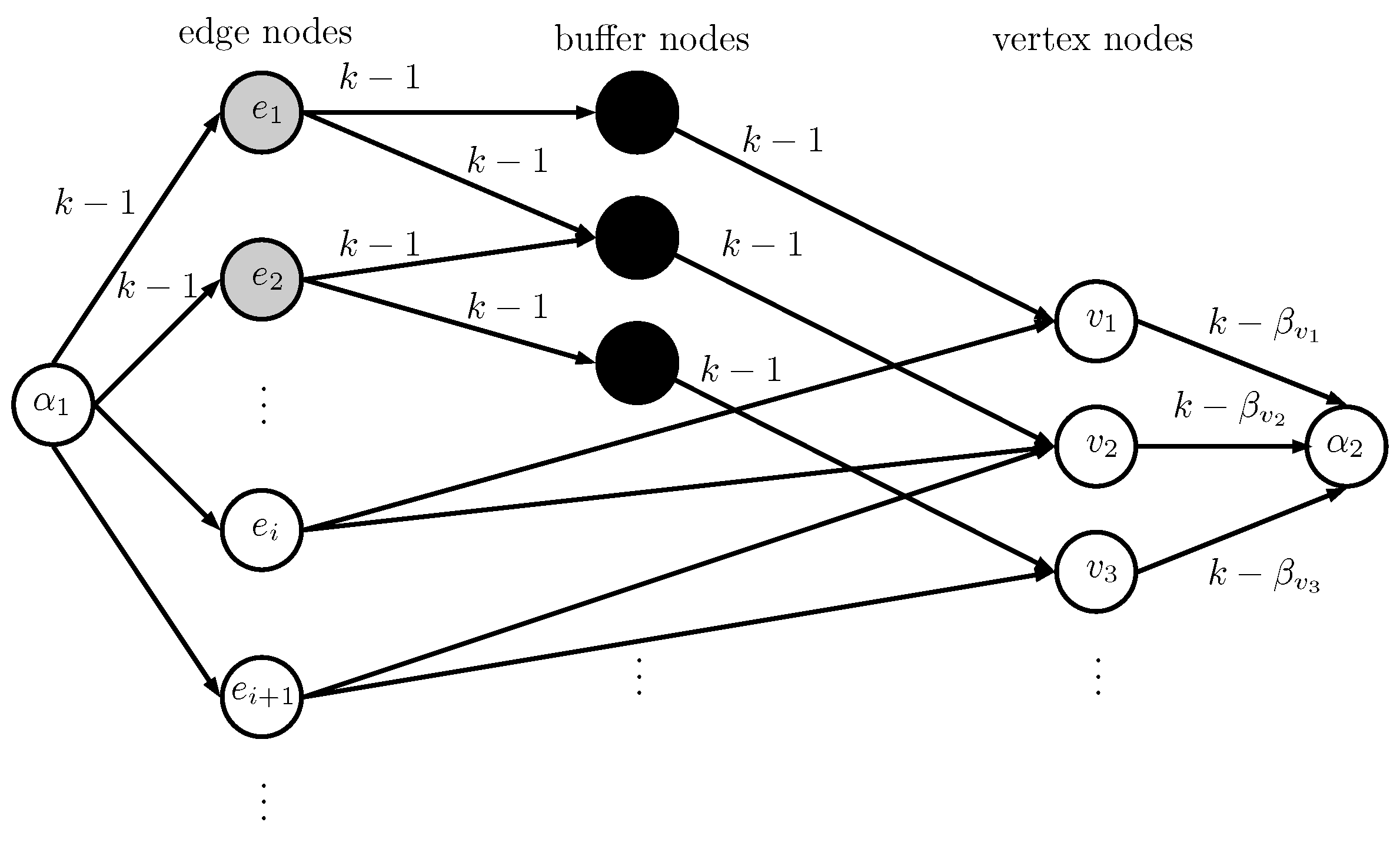The algorithm will build a modified version of the flow network N of Lemma 2, which we describe now. First, change the capacities on the arcs incident on the big edge nodes from k to $k-1$. Second, for each $v\in V$, set the capacity of the arc from buffer node v to vertex node v to $k-1$ instead of k. Leave the capacities from the vertex nodes to the sink ${\alpha }_2$ as $k-{\beta }_v$. We show this flow network in Figure 2. It is straightforward to see that this modified network maintains the same property that all the arcs leaving ${\alpha }_1$ are saturated in an integral maximum flow if $OPT\le 1$.

We modify the algorithm from Lemma 2 as follows. We refer the reader to BigSmall_$rs$ (Algorithm 3). The modified flow network we described above is built for Step 1. Steps 2–3 are the same as before. In Step 4, when constructing the bipartite graph $G^{\prime }$ between the big edge nodes and buffer nodes, $V_{big}$ remains the same, but $V_{rec}$ contains buffer nodes that receive instead at least $\lceil (k-1)/2\rceil$ units of flow from a big edge node and

$$E^{\prime }=\left\{(u,v)\right|u\in V_{big},v\in V_{rec},f(u,v)\ge \lceil (k-1)/2\rceil \}$$

steps 5–8 remain the same as before. Since the capacities of the arcs leaving the buffer nodes and the incoming flow to the big edge nodes are one less than in the network in Lemma 2, one can show a matching on $G^{\prime }$ exists if $OPT\le 1$ by replacing k with $k-1$ and switching the even and odd cases of our original argument in Lemma 2.

Consider the load of a vertex v in the orientation produced by the algorithm. Clearly any vertex v with $q_v\ge r+s$ has ${\beta }_v=k$ and $k-{\beta }_v=0$. No flow is sent to these vertex nodes, so the load of these vertices is at most 1. Now, examine vertices with $0\le q_v<r+s$. If $q_v\ge s$, then at most one additional small edge can be oriented towards v. Hence, the load of v when $q_v\ge s$ is at most $q_v+r\le 1+r\le 3/2$ since $r\le 1/2$. Finally, consider when ${\beta }_v=p_v$ and $q_v=p_{v}r<s$.

• Let v be a vertex with a big edge oriented towards it. At least $\lceil (k-1)/2\rceil$ units of flow are sent from its big edge node to v. Then, at most $(k-p_v)-\lceil (k-1)/2\rceil$ small edges can be oriented along with the big edge towards v.
• Let v not have a big edge oriented towards it. At most $k-p_v$ small edges are oriented towards v.

Therefore, the load of v is at most

$$\begin{array}{c}{p}_{v}r+max\{r(k-p_v),s+r((k-p_v)-\lceil (k-1)/2\rceil )\}\hfill \\ \le max\{rk,s+r(k-(k-1)/2)\}\hfill \\ <max\{k/k,k/(k+1)+(k+1)/2k\}\hfill \\ =k/(k+1)+1/(2k)+1/2\hfill \\ <(k+1)/(k+1)+1/2=3/2\hspace{1em}☐\hfill \end{array}$$

2.4. Step 5.3

For the final case in Step 5 of our algorithm, we apply a variant of the algorithm by Ebenlendr et al. [7]. First we give a brief explanation of their original algorithm that has approximation ratio $7/4$.

Let $E^B$ be the set of big edges and let $G^B=(V,E^B)$ be the subgraph of G consisting of big edges. If $OPT\le 1$, every connected component of $G^B$ with b vertices contains at most b edges, which implies that each component has at most one cycle. For each connected component, identify a cycle if it exists, then orient every big edge not in the cycle away from the cycle and remove each oriented edge. Add the weight of each oriented big edge to the dedicated load of the endpoint farther from the cycle. $G^B$ is now a disjoint union of trees and cycles.

As shorthand, if v is a vertex and e is an edge, $v\in e$ means “v is incident to e”. For any $T\subseteq G$, let

$$L(T)=\{(v,e)\in V\times E|v\text{is}\mathrm{a}\text{leaf}\text{of}T,v\in e,\text{and}e\in T\}$$

where each $(v,e)$ is called a leaf pair of T. Consider any tree $T\subseteq G^B$. Assuming $OPT\le 1$, since T has one more vertex than edges, at most one edge in the set of leaf pairs can be oriented away from its leaf. This leads to what is called the tree constraint (Tree T) in linear program 1 (LP1) shown below, which is a relaxation of an integer program formulation of the graph balancing problem. A variable $x_{ev}$ is defined for each edge $e\in E$ and endpoint v of e. If $x_{ev}=1$, e is oriented towards v. If $0<x_{ev}<1$, we say that e is fractionally oriented towards v.

Linear program 1 (LP1)

$$\begin{array}{ccc}\hfill x_{eu}+x_{ev}=1& \hfill \text{for}\text{all}e=\{u,v\}\in E& \hfill \\ \hfill q_v+\sum _{e|v\in e}{p}_e{x}_{ev}\le 1& \hfill \text{for}\text{all}v\in V& \hfill \\ \hfill \sum _{(v,e)\in L(T)}{p}_e{x}_{ev}\ge \sum _{(v,e)\in L(T)}{p}_e-1& \hfill \text{for}\text{each}T\subseteq G^B& (\text{Tree}T)\hfill \\ \hfill x_{ev}\ge 0& \hfill \text{for}\text{all}e\in E\text{and}v\in e.\end{array}$$

Solve LP1 to obtain a fractional solution $\mathbf{x}$. As a brief remark, there can be exponentially many trees, but there is a separation oracle that can be used to solve LP1 in polynomial time with the ellipsoid method [7]. Let $E_x=\{e\in E|0<x_{eu}<1\text{for}u\in e\}$. Also, let $G_x=(V,E_x)$ and $G_x^B=(V,E_x\cap E^B)$. If a feasible solution is not found for LP1, then $OPT>1$.

The algorithm then considers fractionally oriented edges in $G_x$, and performs a rounding procedure to determine their final orientations. It is assumed that as edges are oriented, $G_x$ and $G_x^B$ are updated accordingly. If there is a vertex v of degree 1 in $G_x$ and $0<x_{ev}<1$ for edge $e=\{u,v\}$ then

• Leaf assignment: if $p_e{x}_{eu}\le 3/4$, e is oriented towards v;
• Tree assignment: if $p_e{x}_{eu}>3/4$ note that e then is a big edge and the connected component of $G_x^B$ containing e must be a tree T. Orient all edges in T away from v.

Finally, if no vertex v as above is found, then there must be a cycle. If so, perform a walk around the cycle changing the values $x_{eu}$ of the edges in the cycle by the minimum amount δ that makes at least one of these values zero and the loads on the vertices remain unchanged. Note that when traversing $G_x$ to find a cycle, big edges are taken in priority over small edges. This step is called rotation. The algorithm terminates once $G_x$ no longer has an edge.

The rounding performed by a leaf assignment increases the load of a vertex u by at most $3/4$ if the edge e under consideration is big or it increases by at most $1/2$ if e is small. Furthermore, a tree assignment can increase the load of a vertex u by at most $1/4$. A vertex u can have its load increased by either only one leaf assignment or by a tree assignment plus a leaf assignment involving a small edge. In either case the maximum load of a vertex is at most $7/4$. Note that a rotation does not change loads.

Now we show how to modify this algorithm for our problem.

Lemma 4. 

For every positive integer $k\ge 2$, there is a polynomial-time algorithm for the graph balancing problem with two rational weights $r,s$, where $1/(k+1)<r\le 1/k$ and $1/2<s<(k-1)/k$ that either finds a solution of value at most $3/2$ or proves that $OPT>1$.

Proof. 

We make the following modifications to the algorithm in [7]. Consider any tree $T\subseteq G^B$. Every big edge e has weight $p_e=s$, so we simplify the tree constraint to

$$\sum _{(v,e)\in L(T)}s{x}_{ev}\ge \left(\sum _{(v,e)\in L(T)}s\right)-s\iff \sum _{(v,e)\in L(T)}{x}_{ev}\ge \left|L(T)\right|-1$$

Also, in the rounding procedure of [7] we change the leaf assignment and tree assignment:

• New leaf assignment: if $p_e{x}_{eu}\le 1/2$, e is oriented towards v.
• New tree assignment: if $p_e{x}_{eu}>1/2$, then e is a big edge and the connected component of $G_x^B$ containing e is a tree T. Orient all edges in T away from v.

Use the algorithm of Ebenlendr et al. [7] with the above modifications. If no fractional solution is found then no orientation exists; report FAIL if this is the case. Since modifying the above threshold from $3/4$ to $1/2$ will still allow all fractionally oriented edges to be rounded, the algorithm still finds an orientation in polynomial time.

We can extend the arguments by Ebenlendr et al. [7] to show that the algorithm has approximation ratio $3/2$ in our case. It is not hard to modify the proof of Theorem 1 in [7] to show that the following conditions are maintained by each vertex $v\in V$ before and after each step in the rounding procedure.

(1)

The load of v is at most $3/2$.

(2)

If $e\in G_x$ is incident on v, then v has load at most $1+(s-1/2)$.

(3)

If $e_B$ is a big edge in $G_x^B$ incident on v, the load of v is at most 1.

(4)

For any tree T that is a subgraph of $G_x^B$, the tree constraint (Tree T) is never violated.

For completeness we sketch a proof that the above conditions hold throughout the rounding procedure. At the beginning of the algorithm, after the modified LP1 is solved, all the conditions above are satisfied and the load of each vertex is at most 1. Next, we show conditions (1)–(4) are preserved for any vertex that changes its load during the rounding procedure.

• Tree assignment: In a tree assignment, only vertices in the tree $T\subseteq G_x^B$ containing big edge $e=\{u,v\}$ for which $p_e{x}_{eu}>1/2$ and v is a leaf of T have their loads modified. Every vertex in T is incident with a big edge in $G_x$. Hence before this step is performed, by condition (3), each one of these vertices has load at most 1. Consider vertex $u^{\prime }$ in T after the tree assignment has been performed. If $u^{\prime }=v$, the load of v is decreased as big edges are oriented away from v. If $u^{\prime }\ne v$, there exists a path P in T from $u^{\prime }$ to v. Say this path begins at edge $e^{\prime }$. As P is a subtree of T, it must satisfy our tightened tree constraint of LP1 and so

  $$x_{ev}+x_{e^{\prime }{u}^{\prime }}\ge \left|L(P)\right|-1=2-1=1\iff x_{e^{\prime }{u}^{\prime }}\ge (1-x_{ev})=x_{eu}$$

  All the edges in P are big, so $s{x}_{e^{\prime }{u}^{\prime }}\ge s{x}_{eu}>1/2$. Hence, the load of $u^{\prime }$ increases by at most $s-s{x}_{e^{\prime }{u}^{\prime }}<s-1/2$, and conditions (1) and (2) are satisfied for vertex $u^{\prime }$. Note that since fractional edge assignments in T have been eliminated, $u^{\prime }$ cannot be incident on a big edge following a tree assignment. Thus, condition (3) does not apply to this case and condition $(4)$ is satisfied.
• Leaf assignment: In a leaf assignment, edges are oriented towards a leaf vertex. Say vertex v is a leaf. We consider two cases for edge $e=\{u,v\}$ such that $p_e{x}_{eu}\le 1/2$: $p_e>1/2$, and $p_e\le 1/2$.
  If $p_e>1/2$, then v is incident on a big edge and so by condition (3), the load of v is at most 1 before the leaf assignment. Since $p_e-x_{ev}{p}_e=x_{eu}{p}_e\le 1/2$, then following the leaf assignment, the load of v is at most $1+1/2=3/2$.
  If $p_e\le 1/2$, then $p_e=r$. By condition (2), before the leaf assignment the load of v is at most $1+(s-1/2)$. So after the leaf assignment the load of v is at most

  $$1+(s-1/2)+r\le 1+(k-1)/k-1/2+1/k=3/2$$

  In any case, after a leaf assignment v is isolated in $G_x$, so conditions $(1)$–$(4)$ are satisfied.
• Rotation: The rotation step does not change the vertex loads so conditions (1)–(3) hold. The argument showing that condition (4) holds is essentially the same as that in [7] and since it is a bit lengthy we omit it here.

Therefore, by condition (1), the load of a vertex is at most $3/2$.  ☐

2.5. Proof of Approximation Algorithm

Finally we prove our algorithm is indeed a $3/2$-approximation algorithm for GBP2W.

Theorem 5. 

There is a $3/2$-approximation algorithm for the graph balancing problem with two weights.

Proof. 

Recall that in Step 1, algorithm GB2W scales the edge weights and vertex dedicated loads by T, then sets $T=1$. Step 3 of algorithm GB2W invokes the algorithm of Lenstra et al. [2]. This algorithm finds a fractional solution using linear programming, and then it performs a two-step rounding procedure. If the value of an optimum solution is $OPT\le 1$, the first step guarantees that the load of any vertex is at most 1; the second step orients at most one more edge towards each vertex. Hence, either an orientation with maximum load $1+max\{r,s\}\le 1+1/2=3/2$ is found, or $OPT>1$ and an orientation is not produced. For Steps 4 and 5 of algorithm GB2W, Lemmas 1–4 ensure that either a solution of value at most $3/2$ is found or $OPT>1$. Therefore, if $OPT\le 1$, Step 6 of the algorithm returns an orientation γ; otherwise it returns FAIL.

The binary search then is guaranteed to find a value $T\le OPT$ and an orientation with load at most $3T/2$. For a weighted multigraph $G=(V,E,\mathbf{p},\mathbf{q})$, since $OPT\le \left|E\right|s$, the number of iterations of the binary search is at most $O(log\left|E\right|+logs)$ and since algorithm GB2W has polynomial running time, the overall running time is also polynomial in the size of the input.  ☐

3. Conclusions

We have presented a 3/2-approximation algorithm for the graph balancing problem with two weights, which meets the best-known inapproximability bound 3/2. We hope our result further motivates other researchers to investigate the 3/2 to 2 inapproximability-to-approximation gap for the makespan minimization problem on unrelated parallel machines.

References

1. Graham, R.L.; Lawler, E.L.; Lenstra, J.K.; Kan, A.R. Optimization and approximation in deterministic sequencing and scheduling: A survey. Ann. Discrete Math. 1979, 5, 287–326. [Google Scholar]
2. Lenstra, J.K.; Shmoys, D.B.; Tardos, É. Approximation algorithms for scheduling unrelated parallel machines. Math. Program. 1990, 46, 259–271. [Google Scholar] [CrossRef]
3. Shchepin, E.V.; Vakhania, N. An optimal rounding gives a better approximation for scheduling unrelated machines. Oper. Res. Lett. 2005, 33, 127–133. [Google Scholar] [CrossRef]
4. Gairing, M.; Monien, B.; Woclaw, A. A faster combinatorial approximation algorithm for scheduling unrelated parallel machines. Theor. Comput. Sci. 2007, 380, 87–99. [Google Scholar] [CrossRef]
5. Asahiro, Y.; Jansson, J.; Miyano, E.; Ono, H.; Zenmyo, K. Approximation algorithms for the graph orientation minimizing the maximum weighted outdegree. J. Comb. Optim. 2011, 22, 78–96. [Google Scholar] [CrossRef]
6. Chakrabarty, D.; Khanna, S.; Li, S. On (1, ε)-restricted assignment makespan minimization. In Proceedings of the Twenty-Sixth Annual ACM-SIAM Symposium on Discrete Algorithms, San Diego, CA, USA, 4–6 January 2015; pp. 1087–1101.
7. Ebenlendr, T.; Krčál, M.; Sgall, J. Graph balancing: A special case of scheduling unrelated parallel machines. Algorithmica 2014, 68, 62–80. [Google Scholar] [CrossRef]
8. Kangbok, L.; Leung, J.Y.-T.; Pinedo, M. A note on graph balancing problems with restrictions. Inf. Process. Lett. 2009, 110, 24–29. [Google Scholar]
9. Kolliopoulos, S.G.; Moysoglou, Y. The 2-valued case of makespan minimization with assignment constraints. Inf. Process. Lett. 2013, 113, 39–43. [Google Scholar] [CrossRef]
10. Page, D.R. Approximation algorithms for subclasses of the makespan problem on unrelated parallel machines with restricted processing times. SOP Trans. Appl. Math. 2015, 2, 20–27. [Google Scholar] [CrossRef]
11. Svensson, O. Santa claus schedules jobs on unrelated machines. SIAM J. Comput. 2012, 41, 1318–1341. [Google Scholar] [CrossRef]
12. Vakhania, N.; Hernandez, J.A.; Werner, F. Scheduling unrelated machines with two types of jobs. Int. J. Prod. Res. 2014, 52, 3793–3801. [Google Scholar] [CrossRef]
13. Verschae, J.; Wiese, A. On the configuration-LP for scheduling on unrelated machines. J. Sched. 2014, 17, 371–383. [Google Scholar] [CrossRef]
14. Ebenlendr, T.; krčál, M.; Sgall, J. Graph balancing: A special case of scheduling unrelated parallel machines. In Proceedings of the Nineteenth Annual ACM-SIAM Symposium on Discrete Algorithms, San Francisco, CA, USA, 20–22 January 2008; pp. 483–490.
15. Asahiro, Y.; Jansson, J.; Miyano, E.; Ono, H.; Zenmyo, K. Approximation algorithms for the graph orientation minimizing the maximum weighted outdegree. In Proceedings of the Third International Conference on Algorithmic Aspects in Information and Management, Portland, OR, USA, 6–8 June 2007; pp. 167–177.
16. Hall, P. On representatives of subsets. J. London Math. Soc. 1935, 10, 26–30. [Google Scholar]
Figure 1. The flow network N for the case when 1 / ( k + 1 ) < r 1 / k and k / ( k + 1 ) s 1 . Shaded nodes represent big edge nodes, and each black node is a buffer node associated with one vertex node. Arcs that are unlabelled have flow capacity 1.
Algorithms 09 00038 g001
Figure 2. The modified flow network constructed for the case when 1 / ( k + 1 ) < r 1 / k and ( k 1 ) / k s < k / ( k + 1 ) . Shaded nodes represent big edge nodes, and every black node is a buffer node associated with a vertex node. Assume arcs that are unlabelled have flow capacity 1.
Algorithms 09 00038 g002