1. Introduction
1.1. A First-Year Student’s Approach to the Vertex Cover Problem
How would a first-year student of computer science approach the problem of choosing at most k vertices from a graph such that all edges have at least one of their endpoints chosen? Most readers will know, of course, that this is an NP-complete vertex cover problem, and you are now most likely mentally weighing the different tools at your disposal for attacking such problems from the vast machinery developed in complexity theory. However, what would our first-year student do? If she is smart, she would first try to apply the arguably most important and ubiquitous algorithmic approach in computer science: divide-and-conquer. After all, she has seen that this approach lies at the heart of fundamental algorithms in computer science (like merge-sort, quick-sort, or binary search), and she has been told that it is also routinely used in advanced algorithms (such as the “search trees of fixed-parameter algorithms”, whatever these may be, she wonders).
1.1.1. Solving Vertex Cover Using Divide-and-Conquer?
Unfortunately, our student quickly notices that the divide-and-conquer approach fails quite miserably when she tries to apply it to finding small vertex covers. The problem lies in the dividing phase: how does one divide, say, a clique into parts? Indeed, divide-and-conquer is only applicable to problems whose inputs are “amenable” to dividing them into parts. Thus, let us make the problem (much) easier for our student by allowing only trees as input graphs. Now, clearly, dividing the input is no longer a problem: For a tree T with root r, we can recurse on the subtrees to rooted at the children to of the root.
Our student must still tackle the merging phase of the divide-and-conquer approach: How does one assemble optimal vertex covers for the into an optimal vertex cover C for the whole tree T? Clearly, this is not a trivial task since the seem to lack some of the information needed for computing C. The trick is to compute two optimal vertex covers and for each subtree : one for the case that the tree’s root is part of the vertex cover and one for the case that it is not. Given these pairs of optimal solutions for each subtree, the best overall solution is of course given by the union of all (since we must cover the edges starting at r), while the best overall consists of r plus the smaller one of or for each i. When our student modifies her divide-and-conquer algorithm so that these pairs are computed, she can solve for the vertex cover problem on trees in linear time.
1.1.2. The Question of Why
Algorithmic metatheorems, which this paper is about, help us in understanding
why the vertex cover problem behaves the way it does with respect to the divide-and-conquer approach. Why does the division phase fail? Why does the merging phase work? Answering the first question seems easy: general graphs do not have any “decomposition property” at all. On the other hand, if the graph is a tree, everything is fine, and it turns out that “everything is
still fine” when the graph is “nearly” a tree, namely a graph of bounded tree width (this concept will be explained in more detail later). Answering the second question seems harder: the answer “because solutions can be assembled using a small trick” does not generalize very well. It took the research community quite some time to find a better answer: In 1990, Courcelle [
1] found that the merging phase works “because the vertex cover problem can be described in monadic second-order logic” (this logic will also be explained in more detail later).
In general, algorithmic metatheorems follow a fixed pattern. They state that problems that can be described in a certain logic (“are amenable to merging” for the right logic) and whose instances can be decomposed in a certain tree-wise fashion (“are amenable to division”) can be solved within a certain amount of time or space. The just-mentioned result by Courcelle is known as
Courcelle’s Theorem (Proposition 6.4, p. 227, [
1]) and states in full (phrased in modern terminology):
all monadic second-order properties of graphs of bounded tree width can be decided in linear time. It was just the first in a long line of further theorems that have been discovered, which basically only vary the three “parameters” of algorithmic metatheorems: the logic, the instance structure, and the required resources. By weakening one of them, one can often strengthen another. For instance, when we use first-order logic instead of monadic second-order logic (which narrows that class of problems considerably since we can express much less in first-order logic compared to second-order logic), we can change the requirement on the decomposition property to, for instance, “nowhere dense graphs” [
2] (a much larger class of graphs than those of bounded tree width) and still obtain a (near) linear time bound or, as a more familiar example, to planar graphs and still obtain a linear time bound [
3]. In another direction, when we increase the time bound to polynomial (rather than linear) time, we can broaden the class of graphs to graphs of bounded clique-width (which is another generalization of bounded tree width) [
4]. In yet another direction, which will interest us in the present paper, it has been shown [
5] that Courcelle’s Theorem also holds when “linear time” is replaced by “logarithmic space”.
1.2. The Range of Applications of Algorithmic Metatheorems
The power of algorithmic metatheorems lies in their ease of application. If our student had known about Courcelle’s Theorem, finding a linear-time algorithm for the vertex cover problem on trees would have been much easier for her: The problem can be described in monadic second-order logic (as we will see later) and trees are clearly “tree-like”, so the theorem tells her (and us) that there is a linear-time algorithm for the problem. Admittedly, the vertex cover problem on trees is not the most difficult problem imaginable from an algorithmic point of view and using Courcelle’s Theorem to solve it might seem like a bit of an overkill, but by the logspace version of Courcelle’s Theorem, we also get a logspace algorithm for this problem for free and coming up with such an algorithm directly is quite difficult (readers are cordially invited to give it a try). Furthermore, we will see that there are many problems that can be formulated in monadic second-order logic, which immediately shows that all of these problems can be solved both in linear time and in logarithmic space on tree-like graphs.
To make the vertex cover problem accessible to algorithmic metatheorems (and to allow our student to apply divide-and-conquer to it), we simplified the problem quite radically: we simply required that the inputs must be trees rather than general graphs. Instead of only trees, algorithmic metatheorems typically allow us to consider input graphs that are only tree“-like”, but this is still a strong restriction. It is thus somewhat surprising that algorithmic metatheorems can also be used in contexts where the inputs are not tree-like graphs. The underlying algorithmic approach is quite ingenious: Upon input of a graph, if the graph is tree-like, we apply an algorithmic metatheorem, and if the graph is not tree-like, it must be “highly interconnected internally”, which we may be able to use to our advantage to solve the problem.
One deceptively simple problem where the just-mentioned approach works particularly well is the
even cycle problem, which just asks whether there is a cycle of even length in a graph (in the graph
![Algorithms 09 00044 i001]()
, the black vertices form the only even cycle). It is not difficult to show that, just like the vertex cover problem and just like about any other interesting problem, the even cycle problem can be described in monadic second-order logic, and thus be solved efficiently on tree-like graphs. Now, what about highly interconnected graphs that are
not tree-like? Do their many edges somehow help in deciding whether the graph has an even cycle? It turns out that the answer is a resounding “yes”: such graphs
always have an even cycle [
6]. In other words, we can solve the even cycle problem on
arbitrary graphs as follows: if the input graph is not tree-like, simply answer “yes”, otherwise apply Courcelle’s Theorem to it.
Naturally, we will not always be so lucky that the to-be-solved problem more or less disappears for non-tree-like graphs, but we will see in the course of this paper that there is a surprisingly large range of problems where algorithmic metatheorems play a key role in the internals of larger algorithms for solving them.
1.3. Intended Audience and Organization of This Paper
This paper, especially the next section, is addressed at readers who are not yet (very) familiar with algorithmic metatheorems and who would like to understand both the basic concepts behind them as well as to see some applications of these theorems in the field of algorithmics and complexity theory. To this purpose, the next section first explains the basic ingredients of Courcelle’s Theorem: What exactly is monadic second-order logic, and how can the concept of being “tree-like” be formalized? Following the exposition of Courcelle’s Theorem, we have a look at three different algorithmic metatheorems and some of their beautiful applications.
No complete proofs of theorems will be presented. These can be found in the literature references, but you will find explanations of the core proof ideas.
1.4. Related Work
Except for the next introductory section, the theorems and applications presented in this paper all concern
small space and circuit classes, even though most algorithmic metatheorems in the literature concern
time classes. The reasons that I chose these theorems are, firstly, that there are already a number of excellent surveys on algorithmic metatheorems and their applications regarding time-efficient computations [
7,
8,
9]. Secondly, the presented theorems are more recent and their applications may thus also be of interest to readers already familiar with algorithmic metatheorems for time classes.
Thirdly, the presented theorems can be used to establish completeness results for many problems for which the classical algorithmic metatheorems do not yield an exact complexity-theoretic classification: using Courcelle’s Theorem and the tricks hinted at earlier, the even cycle problem can be solved in linear time and, clearly, this is also a tight lower bound. However, from a structural complexity-theoretic point of view, the problem is most likely not complete for linear time; indeed, it is complete for logarithmic space and the theorems presented in this paper are useful for establishing such results.
2. The Concepts and Ideas Behind Courcelle’s Theorem
When a theorem can be stated very succinctly and still makes a mathematically deep statement, the reason is usually that the
concepts mentioned in the theorem have complex and careful definitions. This is very much true for the following 17-word-phrasing of Courcelle’s Theorem—but see Proposition 6.4 on page 227 in [
1] for the original formulation—which references two core concepts (monadic second-order logic and bounded tree width) that we now have a look at.
“All monadic second-order properties of graphs of bounded tree width can be decided in linear time.”
2.1. Describing The Problems: Monadic Second-Order Logic
The “meta” in “algorithmic metatheorem” comes from the fact that these theorems do not make a statement about a single algorithmic problem, but apply to a whole range of them—namely, to all problems that can be described in a certain logic. Using logic for describing problems has a long tradition in computer science; indeed, the whole field of
descriptive complexity theory [
10] does little else. As we will see in a moment, this approach has a great unifying power.
2.1.1. The Need for Metatheorems
To better appreciate why we need a unifying framework for talking about some algorithmic results, please have a look at the following quotation from a paper by Bodlaender (pp. 7–8, [
11]) from 1989 (just a year before the first algorithmic metatheorem was presented by Courcelle):
Theorem 4.4 Each of the following problems is in NC when restricted to graphs with tree width , for constant K: vertex cover [GT1], dominating set [GT2], domatic number [GT3], chromatic number [GT4], monochromatic triangle [GT5], feedback vertex set [GT7], feedback arc set [GT8], partial feedback edge set [GT9], minimum mammal matching [GT10], partition into triangles [GT11], partition into isomorphic subgraphs for fixed H [GT12],...
⋮
47 (!) further problems
⋮
...maximum length-bounded disjoint paths for fixed J [ND41], maximum fixed-length disjoint paths for fixed J [ND42], chordal graph completion for fixed k, chromatic index, spanning tree parity problem, distance d chromatic number for fixed d and k, thickness for fixed k, membership for each class C of graphs, which is closed under minor taking.
Researchers desperately wanted to replace such page-long listings of problems with just one phrase: “Each problem that can be described in a certain way is in NC, when restricted to graphs with tree width , for constant K.” The obvious question, which remained unresolved for some time, is of course: What is the “certain way”?
2.1.2. Using Predicate Logic to Describe Problems
Having a look at the list of problems, you will first notice that they are all graph problems. This already indicates a direction in which our logical description should go: First, to simplify matters, we will only consider graphs as inputs, which fits perfectly with the list of problems in the theorem (one can more generally consider arbitrary logical structures, but while this does not add expressive power, it does add unnecessary complications in the context of the present paper). Second, in order to talk about graphs using logic, we need to reference them in logical formulas. We do so by viewing a (directed) graph with vertex set V and edge set as a logical structure in the sense of predicate logic with “universe V” and being a binary relation on this universe. The signature (also sometimes called a logical vocabulary) of the structure is , consisting of a single binary relation symbol. The (first-order) variables of a formula in predicate logic will now refer to vertices: Consider the simple problem of deciding whether all vertices of a graph have an outgoing edge. A graph will have this property if, and only if, , that is, if it is a model of the formula. As another example, the problem of telling whether there is a walk of length 2 somewhere in the graph be expressed using the formula . In general, the set of all (finite) graph models of a formula is said to be the problem described by the formula.
Returning to the list of problems in the quotation, you may also have noticed that they lie in NP and are typically NP-complete. To describe such problems, formulas in first-order logic do not suffice: basically, each first-order quantifier in a formula can be “tested” using a simple parallel for-loop and, thus, first-order formulas can only describe rather simple problems. The great power of the class NP comes from the ability of nondeterministic Turing machines to “guess” not only a single vertex, but rather a whole set of vertices. For instance, an NP-machine for deciding the problem 3-colorable (decide whether a graph can be colored with three colors so that there are no monochromatic edges) will nondeterministically guess the three color sets and then do a simple test whether it has “guessed correctly”. Translated to the logical setting, we wish to talk about (and guess) whole sets of vertices, which means using second-order variables: They work and behave like additional relational symbols, but they are not part of the signature. Rather, quantifying over them existentially corresponds exactly to guessing a set of vertices (or even a binary relation) using an NP-machine.
As an example, we can express the problem 3-
colorable using the following second-order formula
:
Let us “read this formula aloud”: it asks whether there exists a set R of (red) vertices, a set G of (green) vertices, and a set B of (blue) vertices such that all vertices x have one of these colors and for all edges the two endpoints x and y do not have the same color.
As another example, let us express the problem
graph-automorphism, which asks whether a graph
G is isomorphic to itself via some isomorphism that is not the identity. This property can also be described using a second-order formula, where
I is a
binary second-order variable that encodes the sought isomorphism (if
is the isomorphism, we want the relation
I to contain all pairs
for
):
In a similar way, other graph problems in NP can be expressed using second-order formulas that start with “guessing” some vertex sets or relations and then testing whether the guess is correct using a first-order formula. Already in 1974, Fagin realized that this is actually
always the case and Fagin’s Theorem [
12] states that a (graph) problem lies in NP if, and only if, it can be described using an existential second-order formula (“existential” meaning that the second-order variables may only be bound existentially, not universally).
2.1.3. The Need for Monadic Predicates
In view of Fagin’s Theorem and the list of problems in the cited theorem by Bodlaender, “existential second-order logic” seems like a promising candidate for the logic that unifies all of the problems in the theorem. However, it turns out that this logic is not quite what we are looking for.
To see where the problem lies, recall what our student did in the divide-and-conquer approach during the merging phase: Given solutions for the different subtrees of a tree, she devised a way of assembling them into an overall solution. The reason she could do this was that in order to combine several solutions for the subtrees, it only mattered whether or not the roots of these subtrees were part of the optimal vertex cover or not. In other words, there is only a small “interface” between the subtrees that is relevant for the vertex cover problem: the roots. The structure of the solution below the roots can be “forgotten” during the algorithm and has no influence on how the solutions to the subtrees are to be assembled optimally.
Translated into the logical setting, we must be able to check the formula separately on subtrees to and then merge the results into an overall result. Vitally, during the merge, no vertices other than the roots may be of importance. In particular, we cannot test whether certain parts of the trees below the roots match or have some other similarity.
Courcelle observed that it is exactly the non-monadic second-order variables that cause problems. A monadic (or “unary”) second-order variable stands for a set of vertices, while a binary second-order variable represents a second edge set. The difference is illustrated nicely by the two examples from above: for 3-colorable, we only use monadic second-order variables and, indeed, if we have colorings for subtrees, merging them only requires us to look at the colors of the roots (of course, the 3-colorability problem is not very interesting for trees, but will become so for tree-like graphs in the next section). In stark contrast, for the graph automorphism problem, where our formula “guessed” the isomorphism using a binary predicate, we cannot merge automorphisms for the subtrees since the important question is exactly how the inner structures of these trees are related. Indeed, algorithmic metatheorems generally fail to apply to auto- and isomorphism problems even though these problems are not even believed to be NP-hard.
To sum up, the logic we have been looking for is monadic second-order logic over graphs. We fix the signature to , where the are optional predicate symbols that can be used to encode additional information about the vertices as part of the input. The formulas are first-order predicate logic formulas in which we may additionally quantify over monadic predicate variables and use them as if they were unary relation symbols in the signature (in addition to the , over which we may not quantify). We may quantify both existentially and universally (unlike Fagin’s Theorem, where only existential quantification is allowed). The earlier formula for the 3-colorability problem is a typical example of a monadic second-order formula while the formula for the automorphism problem is not.
2.2. Decomposing the Problems: Tree Decompositions
Many difficult graph problems become very simple when we restrict attention to trees. The 3-colorability problem on trees does not even deserve to be called a “problem”: for all input trees the answer is of course always “sure, all trees are even 2-colorable, so this one is 3-colorable”. Even for the vertex cover problem on trees, our student might also have taken a completely different approach in order to find optimal vertex covers (based on kernelization, even though she probably would not know this): find a node whose children are all leaves, add it to the vertex cover and then remove it and its children; repeat until the tree has no more edges. No matter what logic we use to describe problems, algorithmic metatheorems will not be very useful when they can only be applied to trees.
How can we relax the requirement that the inputs must be trees? The requirement enabled us to merge solutions for the subtrees easily because these subtrees only interface with the rest of the graph at a single vertex: their roots. All information concerning optimal solutions “below” the roots is irrelevant, it is only the root vertex that is connected to the rest. The idea behind tree decompositions is simply to replace the single vertex over which all information must flow by a small fixed number of vertices. Naturally, the difficulty now lies in defining how several vertices can “block information from fleeing from a subgraph to the larger graph” and how they do this in a “tree-like” fashion.
For this, we use a game.
2.2.1. The Scotland Yard Game
The game is reminiscent of the board game Scotland Yard where k detectives try to catch a thief on a map of London, but we of course play it on our input graph rather than in London (as in the board game, we forget about the direction of edges). At the beginning of the game, the detectives are all at a single vertex (at Scotland Yard) while the thief can choose any vertex of the graph as starting point. Now, both the thief and the detectives can move along edges of the graph and, as in the board game, whenever a detective and the thief are on the same vertex at any given moment, the thief immediately loses. On the other hand, while a detective is traveling from one vertex to another along an edge, she cannot catch the thief. Additionally, the thief can travel very quickly and he can make an arbitrary number of moves while a detective travels.
The thief of course corresponds to the information that we trying to keep boxed in, the detectives correspond to the vertices that “block” the information and that must be taken into account during a recursion.
Let us have a look at how two detectives, Alice and Bob, can catch a thief, Charlie, on a tree such as the one shown left in
Figure 1. Suppose Scotland Yard is at the node
a with Alice and Bob starting there and suppose Charlie starts at node
h. Now, Bob moves from
a to
g, but Alice stays at
a. Charlie need not move in this case, but he could move to any node in the subtree rooted at
g. Suppose he does not move. Next, Bob stays at node
g while Alice moves from
a past him to node
h, forcing Charlie to move away from there. Since he cannot move past Bob on
g, he has to move somewhere downward, say to
m. Now it is Bob’s turn once more, who moves past Alice from
g to
i. Charlie gets a bit panicky at this point and uses his last chance to quickly move from
m to
j before Bob arrives at
i. Naturally, Alice can now move to
j, forcing Charlie further downwards to either
k or
l. Finally, Bob catches Charlie by moving to his position.
In a second example, consider a ring such as the one shown right in
Figure 1. This time, Alice and Bob starting at
a will have a much harder time catching Charlie—more precisely, they cannot: they can endlessly chase him around in circles, but will not catch him if he moves sensibly. Thus, suppose Alice and Bob enlist the help of Dave, a third detective who also starts at
a. The three detectives can catch Charlie in as little as three steps: first, Dave moves to
e, forcing Charlie into either the left or the right half of the circle. Say, he moves to
d. Second, Alice moves to the middle vertex of the half Charlie chose, that is, to
c, forcing him either to
b or to
d. If he moves to
b, Dave can catch him there, if he moves to
d, Bob can.
2.2.2. Decompositions Are Game Strategies
For the first graph, the tree,
two detectives have a “winning strategy” for catching Charlie, no matter where he starts. For the second graph, the cycle,
three detectives have such a strategy (but two do not). The strategies can be described as
trees whose nodes contain sets of positions of the detectives during their hunt for Charlie: at the root, all detectives are at Scotland Yard. For a positioning of the detectives, the children of this position in the tree are the next positions for the detectives, depending on where Charlie might be.
Figure 2 shows the strategy of the three detectives for the cycle graph with black vertices denoting positions where the detectives are. The mathematical terminology for these strategies is, of course, different: The “strategy trees” are known as
tree decompositions of the graph. For each node of the tree, the set of positions where the detectives are is called the
bag of the node. These bags contain exactly the vertices along which information might “flee” from a smaller subgraph towards the root.
During a divide-and-conquer algorithm, we (only) need to keep track of the vertices in bags and consider (only) all possible ways in which they can be part of an optimal solution. Indeed, the runtime of algorithms that “walk up the tree decomposition” is typically linear in the size of the tree, but exponential in the size of the bags, making the number of detectives needed a crucial parameter.
It is no coincidence that two detectives are needed to corner Charlie on a tree while three are necessary on a cycle: a graph is a tree if, and only if, two detectives suffice. For this reason, the number of detectives minus one is called the tree width of the graph. The tree width of a tree is then 1, the tree width of a cycle is 2, while the tree width of the n-vertex clique is .
Let me make two observations concerning possible strategies of the detectives: First, if necessary, the detectives can always adapt their strategy so they never need to “return” to a vertex that they have left earlier, since they only leave a vertex when Charlie is cornered into an area of the graph from which the left vertex is no longer accessible to Charlie. This means that when we have a look at all nodes of the tree decomposition tree whose bags contain a certain vertex (like the Scotland Yard vertex), these nodes will form a connected component of the tree. Second, for each edge of the graph there will be a bag containing the two endpoints of this edge since, otherwise, Charlie could always go back and forth along this edge without ever being caught.
2.2.3. Defining Decompositions
It turns out that not only do sensible and correct strategies always have the two properties (called the “connectedness property” and the “covering property”), a tree together with bags having them is essentially already a strategy for catching Charlie: Suppose the detectives are positioned at the vertices of a bag of a node n of T and suppose Charlie is on a certain vertex . Charlie is restricted to the vertices u that are reachable from v in . By the connectedness property, the nodes of T that contain a given u form a connected subset of T. By the covering property, the union of these subsets is still a connected subset of T. This means that this union is completely below a single child of n. By moving to the positions in the bag of that child, our detectives will eventually catch Charlie.
To sum up, the easiest way of
defining game strategies is to define a tree decomposition of a graph
as any tree
T with node set
N together with a function
that assigns a
bag to each node
n of
T such that two conditions are met:
Connectedness property: for each vertex, , the set is connected in T.
Covering property: for each edge, , there is a node n with and .
The width of a tree decomposition is the maximum size of any bag in it minus one. The tree width of a graph is the minimum width of any tree decomposition for it. We have already seen that the tree width of a tree is one, the tree width of a cycle is two, and the tree width of an n-vertex clique is .
2.3. The Proof Ideas for Courcelle’s Theorem
With all the ingredients prepared, we can now have a closer look at Courcelle’s Theorem, which has already been mentioned repeatedly. It states:
Courcelle’s Theorem. Let φ be a formula in monadic second-order logic and let be a number. Then, the language and has tree width at most can be decided in linear time.
Proof Ideas. Suppose (a string encoding of) a graph
is given as an input. The first step is to determine a tree decomposition, that is, to find a strategy for the
detectives. One can find such a strategy in time
by iteratively “cutting off” escapes routes for Charlie, but finding such a strategy in
linear time is not so easy. Indeed, the theorem stating that this is, indeed, possible has a dedicated name: it is Bodlaender’s Theorem [
13]. In the following, we will see further examples where the “really difficult part” of an algorithmic metatheorem is finding the tree decomposition.
Suppose we have determined a width-k tree decomposition of . We face the problem that φ refers to , but our recursion should use T instead. One can proceed in different ways at this point, but one elegant way of solving the problem is to modify ϕ so that it refers to T instead of : Very roughly speaking, when φ refers to a variable x standing for a vertex v of , we instead use a second-order variable X that stands for the subset of T’s nodes whose bags contain v; and when φ uses the atomic formula “” to test whether there is an edge between x and y in , we instead test whether there is a node n contained in both X and Y that contains the edge. The modification yields a new monadic second-order formula with the property where is (a logical structure encoding) T together with additional labels representing information about the bag structure. As an example, for the concrete case of φ expressing that G is 3-colorable, expresses something like “there exists a way of assigning the three colors to the vertices of each bag such that the assignment is consistent across all bags containing the same original vertex and nodes whose bags contain the two endpoints u and v of an edge of G must assign different colors to u and v”.
The last step is to determine in linear time whether holds. We use a tree automaton for this: this is a finite automaton that starts its work at the leafs of a tree in some initial state and whose state at a given node depends on the states reached at the node’s children and on the label of the node. Whether the automaton accepts or rejects an input tree depends on the state reached at the root. The automaton for deciding can be constructed by induction on the structure of : atomic formulas just test whether nodes have certain labels; the logical conjunction corresponds to taking the product automaton; the negation corresponds to taking the complement automaton; and a monadic existential quantification corresponds to guessing a labeling using nondeterminism.
Note that both the transformation of φ into a formula and also that of into a tree automaton can be done “in advance”: they do not depend on the input, only on φ and k. During an actual run of the algorithm, we “just” need to compute a tree decomposition and then run a tree automaton on it. ☐
2.4. A Look at the Hidden Constants
Before we proceed, a word of caution might be in order: Courcelle’s Theorem is a beautiful theorem, and in the course of this paper we will see that it also has beautiful applications, but there is a catch (as they say, there is no such thing as a free lunch): the “hidden constants” in Courcelle’s Theorem are huge, and naïvely implementing the algorithms implied in the theorem leads to more or less useless implementations.
The huge constants come from two sources: first, in the proof, I wrote that computing tree decompositions “in linear time is not so easy”, but by Bodlaender’s Theorem “this is, indeed, possible”. It would be more honest to replace this by “in linear time is extremely difficult” and “this is, barely, possible”. Using Bodlaender’s Theorem, we can compute a tree decomposition of an n-vertex graph of tree width k in time for some polynomial p, but p is a high-degree polynomial that yields ridiculously large values already for .
Things get worse, however, for a second reason. Recall that once we have computed the tree decomposition T, we run a tree automaton on it that arises from the formula as follows. Starting from automata for checking atomic formulas, we build more complicated automata recursively: logical conjunctions correspond to taking products; negations correspond to complements; and monadic existential quantifications correspond to nondeterminism. It is well-known in automata theory that complements and nondeterminism do not get along very well or, phrased more scientifically, in order to complement a nondeterministic automaton, we first have to turn it into a deterministic automaton. This means that when starts with something like , each additional quantifier will cause an additional exponential blow-up of the size of the automaton. All told, the automaton will have a size that can only be described by a “tower of exponentials” whose height is given by the length of .
Against the background of these sobering observations, there is some good news and some bad news. FIrst, the bad news—the just-mentioned tower-of-exponentials arising in the algorithm
cannot be avoided: It is shown in [
14] that there is a family of problems on
trees (so the difficulty of computing the tree decompositions does not even arise) that can be described by monadic second-order formulas
φ, but that cannot be decided faster than within a tower-of-exponentials in the length of each
φ.
The good news is that in many practical situations, once it has been established using Courcelle’s Theorem that some problem can be solved in linear time in principle, a closer look at the problem often yields simpler, and much faster, direct solutions for the problem. We will see an instance of this effect later on when we have a look at the unary subset sum problem.
3. An Algorithmic Metatheorem for Logspace and Its Applications
When one is only interested in the deterministic, sequential time complexity of problems, one cannot really improve on Courcelle’s Theorem: in sublinear time, we cannot even read the whole input, let alone do computations depending on all parts of it. However, we may also ask how quickly a problem can be solved in parallel or how much space is needed or even how much energy is necessary—or inquire about any number of further resources.
Concerning parallel time, by rephrasing the lengthy Theorem 4.4 of Bodlaender quoted earlier using the ideas of the previous section (namely, to replace the endless list of problems by the phrase “problems describable in monadic second-order logic”) and having another look at the proof of the theorem, one can show that Courcelle’s Theorem also holds when we replace “linear time” by “polylogarithmic parallel time.” In other words, there is a “parallel time version” of Courcelle’s Theorem.
Naturally (at least, readers familiar with classical computational complexity theory will find this natural), when a problem can be solved quickly in parallel, it can also typically be solved with very little space. This leads to the question of whether we can modify the arguments used by Bodlaender to establish a “logspace version” of Courcelle’s Theorem. The answer is “yes”, but finding the proof took until 2010:
Theorem 1 (Elberfeld, Jakobi, T, 2010, [
5]).
Let φ be a formula in monadic second-order logic and let be a number. Then, the language and has tree width at most can be decided in logarithmic space. Before we have a look at the proof ideas in a moment, let me just give you a one-paragraph refresher of logarithmic space: In this machine model, the input is “read only” (like a “cd-rom”, although our first-year student probably has never heard of them) and the amount of read–write memory available is when the input has length n. This extremely small amount of memory can equivalently be thought of as a constant number of “pointers” or “one-symbol windows” into the input. Despite being a very restricted model, one can do addition, multiplication, and even division in logarithmic space, evaluate Boolean formulas, solve the reachability problem on undirected graphs, and even test whether a graph is planar. Problems that cannot be solved in logarithmic space—unless, of course, certain complexity class collapses occur—include the reachability problem for directed graphs, evaluating Boolean circuits (instead of formulas), or the 2-sat problem (the satisfiability problem for propositional formulas in conjuctive normal form where all clauses have at most two literals). All problems that can be solved in logarithmic space can be solved in logarithmic parallel time (for appropriate models of parallel time) and also in polynomial (but not necessarily in linear) sequential time.
Proof Ideas. Recall that the proof of Courcelle’s Theorem from the previous section proceeded in four steps:
Compute a tree decomposition of the input graph G.
Transform the formula φ into a formula .
Transform the formula into a tree automaton A.
Run A on T.
Clearly, the second and third step work exactly the same way in the logspace setting as in the linear time setting (or, for that matter, in any other setting) since these transformations are independent of the input and can be done in advance. The fourth step, running the tree automaton, is essentially just an elaborate version of evaluating a Boolean formula tree (only, instead of passing the two possible results “true” or “false” towards the root, we pass states) and it is well-known that this can be done in logarithmic space; indeed, it can be done in NC
, a subclass of logarithmic space, as was shown by Buss [
15] already in 1987.
This leaves the first step and, as in the proof Courcelle’s Theorem, computing the tree decomposition is the hard part. Different, rather sophisticated algorithms for computing tree decompositions had been developed, but researchers grew more and more frustrated when trying to analyze their space consumption: they all used way too much space. Michael (Elberfeld) had the key insight at the end of 2009: instead of trying to modify these clever algorithms, let us have a look at the “trivial” way of finding tree decompositions, namely by starting with some root bag (“at Scotland Yard”) and then successively cutting off escape routes. This simple method had been one of the first algorithms known for computing tree decompositions, but it needs time and had been superseded by quicker algorithms at the expense of the space consumption.
Naturally, “successively cutting off escape routes” is not quite that simple to do in logarithmic space: you cannot keep track of what you decided earlier on since the number of “positions” or “chosen vertices” a logspace machine can remember is constant. Here, a second trick comes in: we have a look at all possible ways the detectives can be positioned and then check whether one placement corners Charlie better than another. In other words, we build a graph whose vertices are all possible bags and there is an edge from a bag to another if the second bag could be below the first bag in a tree decomposition. Building this graph and testing all possible combinations takes some time (around ), but only very little space since we only need to keep track of the vertices in two to-be-compared bags, for which we need pointers into the input. (Readers not familiar with logarithmic space may ask themselves at this point “But where do you store this graph”?! The answer is “Nowhere! It is just a ‘virtual’ graph whose edges are recomputed on-the-fly whenever needed.”) Now, in this graph, which we dubbed a “descriptor decomposition, one must start at a root vertex (“Scotland Yard”) and recursively pick appropriate next bags that corner Charlie. It turns out that the descriptor decomposition contains all the necessary information for picking these bags using only logarithmic space. ☐
Before we move to applications of the above theorem, the same words of caution are in order as for the linear-time version: There are
huge hidden constants in the described logspace algorithm. The reasons are nearly the same as earlier: First, the logspace analogue of Bodlaender’s Theorem internally uses Reingold’s ingenious algorithm [
16] for the undirected reachability problem, but this algorithm unfortunately hides constants of around
in the
O-notation. Second, since our construction of the tree automata from the formula
φ has not changed, it still will (indeed, must) lead to tree automata of a size that is a tower of exponentials whose height is the length of
φ.
3.1. Applications: Low-Hanging Fruits
The logspace version of Courcelle’s Theorem has two kinds of applications, which I like to call the “low-hanging fruits” and the “high-hanging fruits”. The low-hanging ones are results that we get more or less “for free” by taking any problem to which the classical version of Courcelle’s Theorem is known to apply and then rephrasing the result in this new setting. As an example, here is a typical lemma you can find in a textbook:
Lemma 2. For each k, the set has tree width at most k and G is 3-colorable} can be decided in linear time.
Proof. The property “G is 3-colorable” can be described by a monadic second-order formula. By Courcelle’s Theorem, we get the claim. ☐
Such lemmas transfer very easily to the logspace setting:
Lemma 3. For each k, the set has tree width at most k and G is 3-colorable} can be decided in logarithmic space.
Proof. The property “G is 3-colorable” can still be described by a monadic second-order formula. By the logspace version of Courcelle’s Theorem, we get the claim. ☐
The transfer works very well for 3-colorability and many other problems, but what about the introductory problem of this paper, the vertex cover problem? You may have noticed that I did not present a monadic second-order formula describing this problem (yet). At first sight, such a formula is easy to obtain: reads aloud “there is a vertex cover C such that for all edges one of the two endpoints lies in C”. However, this is not really what we want: we do not wish to know whether a vertex cover exists (of course it does, just take all vertices), but would like to know whether a vertex cover of a certain size exists. This means that C must be a free monadic second-order variable (we remove the quantifier at the beginning of the formula) and we would like to know whether we can choose an assignment to this free variable that, firstly, makes the formula true and, secondly, has a certain size s that is part of the input. Fortunately, it turns out that both Courcelle’s Theorem and its logspace version can be modified so that they also apply to this situation. Let me state the logspace version explicitly:
Theorem 4 (Elberfeld, Jakobi, T, 2010, [
5]).
Let be a formula in monadic second-order logic with a free monadic second-order variable X and let be a number. Then, the language for some with , and has tree width at most can be decided in logarithmic space. Using this more general version, the list of problems that are “low-hanging fruits” becomes rather long: it includes all of the problems in the long list quoted earlier from Bodlaender’s paper; indeed, it is difficult to find a problem that can
not be described in monadic second-order logic. The graph isomorphism problem is one such exception—and, fittingly, the complexity of deciding whether two graphs of bounded tree width are isomorphic was settled only in 2016, see [
17].
3.2. Applications: Special Fruits
Before we proceed to the really advanced applications, there are some “special” applications of the logspace version of Courcelle’s Theorem that concern problems to which one normally does not apply algorithmic metatheorems: problems inside P, the class of problems solvable in polynomial time. Problems such as perfect-matching or reach are normally considered “easy” since they already lie in P, and, thus, applying an algorithmic metatheorem to them will not move them from “unsolvable” into the realm of “solvable”, but, at best, from “solvable in quadratic or cubic time” to “solvable in linear time with huge hidden factors”—at the expense of making heavy restrictions on the input concerning the tree width. Generally, the expense is considered too high a price to pay and one does not even bother to formulate the resulting statements. However, from the perspective of space complexity, problems like the matching problem belong more to the realm of “unsolvable” problems, and the logspace version of Courcelle’s Theorem does give us useful applications such as the following:
Lemma 5. For each k, the set has tree width at most k and G has a perfect matching} can be decided in logarithmic space.
Lemma 6. For each k, the set has tree width at most k and there is a directed path from s to t in can be decided in logarithmic space.
There is a whole paper ([
18]) mainly devoted just to proving the first lemma directly, which shows nicely how powerful algorithmic metatheorems can be. In both cases, the lemmas follow from the fact that we can describe the graph properties “has a perfect matching” or “there is a path from
s to
t” using monadic second-order logic. (Astute readers may have noticed that monadic second-order logic as defined in this paper does
not allow us to describe the perfect matching problem directly since we would need to quantify existentially over a subset of the graph’s
edges rather than its
vertices. However, this can be fixed easily for instance by subdividing each edge and marking the new vertices using one of the
predicates. Now, existentially quantifying over a subset of these new vertices is essentially the same as quantifying over a subset of the original edges.)
3.3. Applications: High-Hanging Fruits I—Cycle Modularity Problems
The introduction hinted already at applications of algorithmic metatheorems to graphs that do not have bounded tree width. The idea was to develop algorithms that work in two phases: first, we test whether the input graph happens to have tree width at most k for some appropriately chosen constant k and, if so, we use the algorithmic metatheorem to solve the problem. Second, if the graph has tree width larger than k, we use another algorithm that makes good use of this knowledge. This approach is well established in the context of Courcelle’s Theorem and, in some cases, also works for its logspace version:
Theorem 7. The problem even-cycle = { G ∣ G is an undirected graph containing a cycle of even length} can be decided in logarithmic space.
Proof Ideas. There are two core observations needed to prove the theorem: first, we can describe the property “the graph has an even cycle” using monadic second-order logic. We ask whether there exist two (nonempty, disjoint) subsets of the
edges, which we call the red and the green edges, such that each vertex is either incident to none of these edges or to exactly one red and one green edge. (Again, we use the trick of subdividing edges so that we can formally quantify over subsets of the vertices even though we wish to quantify over subsets of the edges.) Second, Thomassen [
6] has proved the following:
There is a number k such that every undirected graph G of tree width more than k has an even cycle.Together, these observations yield the following logspace algorithm for the language even-cycle: Upon input of a graph G, first test whether its tree width is more than k and, if so, accept the input. Otherwise, compute a tree decomposition and run an appropriate tree automaton to decide the problem. ☐
It is worthwhile observing that even-cycle does not only lie in logarithmic space, but is actually complete for it (as can be seen by a simple reduction from the L-complete undirected acyclicity problem: just subdivide each edge). In contrast, the linear time bound on even-cycle resulting from Courcelle’s classical theorem is tight, but even-cycle is not complete for linear time (unless L = P).
The results on the even cycle problem may have made you curious about other problems where the objective is to find a cycle whose length has a certain property (at least, they made me curious). First, the odd cycle problem turns out to be algorithmically easier for the simple reason that if there is a “walk” (unlike a path or a cycle, a walk may contain the same vertex several times) of odd lengths returning to the start vertex, there must be a cycle of odd lengths in the graph. This makes it relatively easy to reduce the odd cycle problem to the undirected reachability problem, which shows that odd-cycle is also complete for logarithmic space.
Second, what about the more general question of whether there exists a cycle in an undirected graph whose length modulo is some number
m is some number
x? The even cycle problem is this problem for
and
, for the odd cycle problem
and
. It turns out that Thomassen’s result holds for
all for
, that is, Thomassen has shown [
6] that
for all there exists a number k such that all graphs of tree width at least k have a cycle whose length modulo m is 0. This means that all “cycle modularity problems” for
are complete for logarithmic space. In sharp contrast, the complexity of this problem for
and
is completely open; the best upper bound is NP!
3.4. Applications: High-Hanging Fruits II—A Refined Version of Fagin’s Theorem
I mentioned Fagin’s Theorem already as one of the cornerstones of descriptive complexity theory: it states that a problem lies in NP if, and only if, it can be described in existential second-order logic (eso-logic). Recall that this logic differs from monadic second-order logic in two ways: we can quantify over binary relations and not only over sets of vertices (which is why the formula describing the graph automorphism problem is allowed), but we can not quantify universally. This means that all eso-formulas can be rewritten equivalently in “prenex normal form”, which, in turn, means that they are of the form for some quantifier-free ψ, some second-order variables (not necessarily monadic), and some first-order variables .
Formulas like from the introduction show that already fragments of eso-logic describe NP-complete problems, in this case a formula with the quantifier prefix . Is this still the case for a shorter prefix like, say, ? The answer is “yes” since, using two quantifiers ( and ), we can “guess” two bits of information for each vertex of a graph, and two bits suffice to describe which of three (even four) possible colors a vertex has. In other words, the quantifier prefix can be used to describe the NP-complete problem 4-colorable. Thus, what about the prefix ? By the same argument, we can describe the 2-colorability problem in this logic, but this is presumably no longer an NP-complete problem, but an L-complete problem. Indeed, it turns out that all problems that can be described by formulas with this prefix already lie in nondeterministic logarithmic space (NL), which is a (presumably small) subclass of P. Naturally, this observation opens a whole box of new questions regarding the expressive power of all the possible quantifier prefixes an eso-formula may have.
Extensive research regarding the expressive power of different quantifier prefixes has climaxed in a 51-page paper [
19] in the Journal of the ACM by Gottlob, Kolaitis, and Schwentick where a dichotomy is proved: for each possible
eso quantifier prefix, it is shown that the corresponding
prefix class (the class of problems expressible by formulas having the given quantifier prefix) either contains an NP-complete problem or is contained in P.
While the NP-hardness results can be obtained by fairly easy reductions from standard problems, the containment results for P are more involved. Indeed, for one particular prefix class, showing containment in P is very difficult: Gottlob, Kolaitis, and Schwentick [
19] spend most of their paper on showing that for all formulas
φ of the form
, where
ψ is quantifier-free, the language
is an
undirected, self-loop-free graph with
lies in P. The authors already observe that their result is probably not the best possible: the languages
equal a special problem “
” in their terminology, and, in their Remark 5.1, they observe “Note also that for each
P,
is probably not a PTIME-complete set. [...] This is due to the check for bounded tree width, which is in LOGCFL (cf. Wanke [1994]) but not known to be in NL”. As this remark shows, the complexity of the prefix class hinges critically on computing tree decompositions. Similarly to our argument for the even cycle problem, the authors also distinguish two cases, namely graphs of large tree width, where special algorithms are applied, and graphs of small tree width, where Courcelle’s Theorem is applied. However, the special algorithms are now somewhat more involved, and it takes considerably more work to use the logspace version of Courcelle’s Theorem to prove the following:
Theorem 8 ([
20]).
Let , where ψ is quantifier-free and contains no relational, function, or constant symbols other than the binary edge relation symbol E. Then, the set is an undirected, self-loop-free graph with can be decided in logarithmic space. To better appreciate the power of this theorem, consider the formula
“Read aloud” this formula asks whether “we can color the vertices of the graph using m colors such that for each vertex x an edge leads to a ‘next’ vertex y with the ‘next’ color”. When a graph satisfies this formula, if we start at any vertex and repeatedly move to the “next” vertex, we will run into a cycle and along this cycle the colors will also “cycle”, which means that the length of the cycle must be a multiple of m. Using this observation, it is not hard to show that a connected undirected graph will satisfy this formula if, and only if, it contains a cycle whose length is a multiple of m for . Since the formula has the prefix required in the theorem, it tells us that all cycle modularity problems for undirected graphs for and can be solved in logarithmic space. Thus, we can prove the earlier observations concerning these problems purely by having a look at the syntax of the formula describing them!
Proof Ideas. The proof of the claim for polynomial time is spread over the 35 pages of
Section 4,
Section 5 and
Section 6 of [
19] and consists of two kinds of arguments: Arguments of a graph-theoretic nature and arguments showing how certain graph problems can be solved in polynomial time. Since the graph-theoretic arguments are independent of complexity-theoretic questions, one only needs to show how the algorithms described in [
19] can be implemented in logarithmic space rather than polynomial time. Here, as in the argument for the even cycle problem, two basic cases are distinguished: either the input graph has sufficiently small tree width (the exact number depends on the formula
φ), in which case one can decide whether
holds using the logspace version of Courcelle’s Theorem, or the tree width is high.
In the latter case, we first preprocess the input graph by removing extra copies of “similar” vertices. Two vertices are “similar” when their neighborhoods are identical, and, if there is a large number of similar vertices, the formula φ cannot distinguish between them any longer and will hold (or not hold) also for the reduced graph. After this preprocessing, we check whether the graph contains some fixed graphs as induced subgraphs (the list of to-be-checked graphs only depends on φ) and can accept, if the graph contains one of them. ☐
The above theorem handles “just” one of the possible quantifier prefixes an
eso-formula can have (albeit the most difficult one) and this prefix yields the class L. What about other prefixes? They can only yield classes inside NP by Fagin’s Theorem, but do some of them yield, say, P? Or NL? Or NC? These questions are answered in [
20], where it is shown that each prefix yields one of the classes NP, NL, L, or FO (first-order logic) and nothing else. In particular,
no prefix yields P, unless NP = P or P = NL.
4. An Algorithmic Metatheorem for Log-Depth Circuits and Its Applications
The proofs of both versions versions of Courcelle’s Theorem, the classical version and the logspace version, proceeded in four steps:
Compute a tree decomposition of the input graph G.
Transform the formula φ into a formula .
Transform the formula into a tree automaton A.
Run the tree automaton A on T.
In both versions, the algorithmically “really difficult” part was the very first step: the computation of the tree decomposition. The next two steps were algorithmically “trivial” in the sense that nothing happens during a run of the algorithm—the transformations are done beforehand and the results get “hardwired” into the algorithm.
Running the tree automaton on a tree is much easier than computing the tree composition, so the last step usually contributes little to the complexity of the algorithms. However, what happens if we make life easier for our algorithms (which seems only fair, considering that we also made life easier for our student) by
providing a tree decomposition of the graph as part of the input? This takes the first step out of the picture and we get an algorithmic metatheorem where the algorithmic complexity hinges (only) on the complexity of evaluating a tree automaton on an input tree, and it was mentioned earlier that Buss showed [
15] in 1987 that this can be done using an NC
-circuit, yielding the following theorem:
Theorem 9 (Elberfeld, Jakobi, T, 2012, [
21]).
Let φ be a formula in monadic second-order logic and let be a number. Then, the language and is a tree decomposition of of width can be decided by anNC
-circuit family. As for logarithmic space, let me give readers less familiar with the class NC a one paragraph review: it is a language class containing problems that can be decided by very shallow circuits, namely circuits of depth for inputs of length n. In the circuits, the usual logical gates (and, or, negation) may be used and these gates must have bounded fan-in, meaning that the and-gates and or-gates may only take two inputs at a time. These kinds of circuits are a good model of fast parallel computations since the gates of a circuit obviously all work in parallel, and, because of the small depth of the circuit, we only have to wait for at most units of time for a decision when we feed an input into the circuit. The problem of evaluating a propositional formula for a given assignment of values to the variables (known as the Boolean formula evaluation problem, BF in short) can be shown to be complete for the class NC. Other problems included in this class are addition, multiplication, and even division. The class NC is a subclass of L and, if it is a proper subclass (as many people believe), problems complete for L like the even or odd cycle problems from the previous section are no elements of NC.
The new requirement we added to Theorem 9, namely that the input graph should be accompanied by a tree decomposition, seems to ruin the whole purpose of the theorem: if the difficult part of proving Courcelle’s Theorem is determining the tree decomposition, then what use could a theorem have that blithely assumes that the tree decomposition is part of the input? It turns out that there are two situations where we do have tree decompositions “handy”. First, even though I claimed in the introduction that considering trees as input is boring and problems only get interesting when the graphs have larger tree width, there are problems on trees that are of interest, and the nice thing about trees is that they are already “their own tree decompositions”. Thus, when our input graphs are trees, we can apply the theorem.
Second, when we produce graphs internally as part of an algorithm, we often have a lot of “control” over this graph, that is, we “know” how it is structured and may sometimes produce a tree decomposition alongside the graph itself. These applications are of course similar to the “high-hanging fruits” from the previous section in the sense that the algorithmic metatheorems are only part of larger algorithms.
4.1. Applications: Model Checking for Propositional Logic
As an application of the first situation, where the input graph is actually a tree, consider the model checking problem for propositional logic: the input is a pair consisting of a propositional formula φ and a variable assignment β that maps each variable in φ to 0 or 1. The question is whether holds. For instance, we might have and and and, clearly, holds.
Lemma 10. The model checking problem for propositional logic lies in NC.
Proof Ideas. First, given a formula
φ as input (coded as a string), one can easily construct a “formula tree
T” that represents
φ (the nodes are labeled ∧ or ∨ or ¬, the leafs are labeled with 0 and 1, depending on what
β tells us about the assignment of the variables), see
Figure 3 for an example.
Now, we want to evaluate the tree using the algorithmic metatheorem. For this, we use a monadic second-order formula stating the following: “Does there exist a subset X of the nodes of the tree such that the following conditions are met: the root is part of X; a leaf is part of X if, and only if, it is labeled 1; a node labeled ∧ is part of X if, and only if, both its children are; a node labeled ∨ is part of X if, and only if, at least one of its children is; and a node labeled ¬ is part of X if, and only if, its child is not”. Clearly, this lengthy formula uses just one monadic quantifier at the beginning and tests whether X contains exactly the nodes of the tree evaluating to 1. ☐
Proving the lemma using the algorithmic metatheorem is, of course, somewhat circular: we used the fact that the Boolean formulas can be evaluated in NC in order to prove the algorithmic metatheorem—so perhaps we should not use it to the prove this very fact and move on to an application that feels less like cheating.
4.2. Applications: Visibly Pushdown Languages
One of the first things one learns in theoretical computer science is that “context-free languages are accepted by pushdown automata”, which more or less settles the complexity of context-free languages from a theoretical point of view. From a practical point of view, however, the fact that these automata can be nondeterministic makes it hard to actually implement them, while at the same time, the full power of context-free grammars is only rarely needed to describe typical parsing problems. For this reason, many different restrictions of context-free grammars and pushdown automata have been studied in the literature, one of which will be of interest to us: the class VPL of visibly pushdown languages, which are the languages accepted by visibly pushdown automata.
The visibly pushdown automata are the same as “normal” pushdown automata, except for one crucial difference: whether such an automaton modifies its stack via a push or a pop or not at all in any given step depends
only on the current input symbol, not on the internal state. As an example, consider a pushdown automaton that checks whether in an input string two different kinds of parentheses (like round and square ones) are correctly balanced, see
Figure 4a for an example. Such an automaton does a
push on all opening parentheses and a
pop on all closing parentheses (and does not modify the stack on other symbols). This is exactly the behavior that a visibly pushdown automaton must have.
Compare such an automaton to the one for the problem of deciding whether in a bitstring the number of 0-bits and 1-bits is the same, see also
Figure 4b: Here, we can use a stack to keep track of the “excess symbols” that we have seen. Whether we need to push or pop the next symbol now depends on whether 0- or 1-bits are currently on the stack and the resulting pushdown automaton is
not a visibly pushdown automaton.
The acceptance problem for visibly pushdown automata (for a fixed automaton A, decide on input w whether A accepts w) may seem quite unrelated to the topic of this section or, for that matter, of this whole paper: this is not even a graph problem! The trick is, of course, that we can construct a graph internally in an algorithm for deciding this acceptance problem, which leads to an elegant proof the following theorem:
Proof Ideas. The first key observation is that for a fixed automaton A and some input word w, the height of the stack reached for any given prefix u of w can be computed very easily: it is the number of symbols of u causing a push minus the number of symbols causing a pop. This means that the overall “shape” or “outline” of the stack during the computation can be computed easily (in a class called “TC”, to be precise) without actually running the automaton.
Next, this “shape” of the stack gives rise to a graph in a natural way as shown on the right: each position where a stack symbol could go is a vertex and edges “connect stack symbols at the same height in adjacent steps”, “fork during a push”, and “join during a pop”. The example graph in
Figure 5 is the one resulting for the automaton for deciding the language of balanced parentheses for the input string
([()()][]).
We make three observations concerning this graph:
It is “easy to compute” since, as explained earlier, the height of the stack at each horizontal position can be computed just by doing a simple subtraction. Clearly, adding the edges is also very easy to achieve.
The graph has tree width 2, that is, three detectives suffice to corner Charlie wherever he might start: two detectives position themselves at the “forking vertex” and at the “joining vertex” of an area containing Charlie and then the third detective moves to an intermediate forking or joining vertex to cut of more of the graph. Note that not only does the graph have tree width 2, we can actually compute the tree decomposition just as easily as the graph itself since this tree decomposition just reflects the nesting structure of the stack.
In order to decide whether the automaton accepts the input word, we use a formula that existentially guesses the contents of the stack at each moment, using unary predicates, and then verifies that the changes of the stack contents along edges are correct (mostly, this means that there may not be any change, except for the top of the stack, where the change must match the automaton’s behavior).
With these three observations, applying this section’s algorithmic metatheorem, Theorem 9, gives the claim. ☐
The containment VPL ⊆ NC
can also be proved directly [
22], but the proof using the algorithmic metatheorem is not only simpler, but generalizes more easily. For instance, just as for logarithmic space, there is also a “counting version” of the theorem and plugging in the same construction as in the above proof yields that counting the number of accepting computations of a visibly pushdown automaton can be done in #NC
—a result that is hard to prove directly [
23].
5. An Algorithmic Metatheorem for Constant-Depth Circuits and Its Applications
In the introduction, we already asked our first-year student of computer science to solve an NP-complete problem (vertex cover), so she probably will not mind when I ask her to help me with two more problems: On a blackboard, I write a lot of rather lengthy natural numbers in small print, allowing me to squeeze, say, 500 numbers on the blackboard. I then ask the student to help me with two tasks: first, circle as few numbers as possible so that their sum is at least a googol (). Second, circle as few numbers as possible so that their sum is exactly a googol.
Our student, being smart, has no trouble with the first task: she repeatedly circles the largest number not yet circled until the sum reaches a googol. Of course, our student
will have trouble with the second task since I maliciously asked her to solve (essentially) the NP-complete problem
5.1. The Unary Subset Sum Problem
Asking our student to solve an NP-complete problem is as unfair as it was in the introduction, so let us make the problem (much) easier once more: suppose I write all numbers in
unary (so instead of 13, I have to write
![Algorithms 09 00044 i002]()
) and to write
in unary, I would need a blackboard larger than the universe. How difficult is the resulting
unary-subset-sum problem? It is easy to see that the problem lies in NL (so it is already much easier than the normal version) and Cook [
24] made an educated guess in 1985 that it is “a problem in NL which is probably not complete”. However, research got stuck at this point and an improvement on the NL bound was only obtained in 2010 when algorithmic metatheorems became available that apply to logarithmic space and the below:
Theorem 12. unary-subset-sum ∈ L.
Proof Ideas. As in the previous section, where we studied visibly pushdown automata, the unary subset sum problem seems to bear no relation to the setting of algorithmic metatheorems (“Where are the graphs?”), but just as in that section, our algorithms will
produce a graph G internally and
apply an algorithmic metatheorem internally. The idea is very simple: upon input
, for each
, we
have a star in G with exactly leafs (and, hence,
vertices). For instance, the input (
![Algorithms 09 00044 i003]()
) gets turned into the following forest of tree width 1 (note that the target number
is not part of it):
![Algorithms 09 00044 i004]()
Consider the formula . We have if, and only if, the set C of vertices “is closed under reachability” or, for the forest graphs above, “each star of the graph is either completely contained in C or not at all”. Now, recall that Theorem 4 stated that there is a logspace algorithm that, upon input of a graph G and the number s, will tell us whether there is a set C with such that holds. In other words, there exists a set C with and if, and only if, there is a set with . ☐
As pointed out earlier, algorithmic metatheorems in general, and the algorithmic metatheorem used above in particular, hide huge constants in the
O-notation and naïve implementations are more or less useless. However, once we know that there is
some logspace or linear-time algorithm, we may try to have a closer look at “what happens” inside the proof and try to extract a simpler, more direct algorithm. This approach works very well for the unary subset sum problem and a reverse engineering of the algorithmic steps leads us to the following algorithm: given distinct numbers
, pick a relatively large
base number
b, for instance
will suffice, and compute the product
We can represent the result as a base-b number: with . Then, the number will be exactly the number of subsets of that sum up to s. In particular, will be an instance of subset-sum if, and only if, .
All told, the unary subset sum problem can be solved by just doing multiplications and extracting certain bits from the result, but we got to this simple algorithm through an analysis of the much more complicated algorithm arising from the algorithmic metatheorem.
5.2. Back to the Original Subset Sum Problem
Considering the unary version of subset-sum instead of the original one may seem a bit like cheating, and, at first sight, the complexity of unary-subset-sum is quite unrelated to the complexity of the “real” subset sum problem. However, it turns out that Theorem 12 actually does tell us a lot about the complexity of the original version:
Corollary 13. subset-sum can be solved by a Turing machine running in pseudopolynomial time and polynomial space.
Proof Idea. Already, our first-year student might know that upon input the subset sum problem can solved using dynamic programming in time , that is, in “pseudopolynomial” time. Unfortunately, the dynamic table needed for this algorithm also has size , that is, we also need pseudopolynomial space. To reduce the space, we do the following: upon inputting , coded in binary, we run the algorithm from Theorem 12 on the same input, but coded in unary. Naturally, that does not really help since we still need space to write down this input, but let us ignore this for the moment.
How much time and space does the run of the algorithm from Theorem 12 need? All logspace algorithms need time polynomial and space logarithmic in the input length. In our case, we need time polynomial in and space logarithmic in . (We can ignore s since the answer is always “no” when it is larger that this sum.) Now, a runtime that is polynomial in is exactly a pseudopolynomial runtime with respect to the input coded in binary, and a space requirement of is a polynomial space requirement in terms of the input coded in binary.
Thus, running the algorithm from Theorem 12 on the input coded in unary has exactly the time and space requirements we are looking for—except that our having to write down the huge unary input spoils the idea. Thus, let us not write down the huge unary input! We turn the unary input into a “virtual tape”: Since the machine we run is a logspace machine, it cannot modify this tape, and whenever the machine tries to read a symbol from this tape, we simply recompute what “would be there if the unary input tape were real” by doing a simple computation on our original binary input. ☐
The above corollary is another example of how algorithm metatheorems can help in simplifying proofs: a direct proof of the above corollary takes up most of a
stoc 2010 paper [
25].
5.3. Bounded Tree Depth
Theorem 12 is not the “final word” on the complexity of the unary subset sum problem. First, observe that it is trivial to compute tree decompositions for the graphs that we construct in the theorem. This means that the hard part of Courcelle’s Theorem—the computation of the tree decompositions—does not need to be performed and Theorem 9 applies (or, rather, an NC-analogue of Theorem 4), yielding unary-subset-sum ∈ NC.
Second, the graphs constructed in the proof of Theorem 12 (the collections of stars) have a special property: not only do two detectives suffice to corner Charlie on a star, no matter how large the star, the two detectives can always corner him in two steps. In other words, we do not only have a strategy for catching Charlie with a bounded number of detectives, but also in a bounded number of steps. Graphs with this property are said to have bounded tree depth:
Definition 14. A class C of graphs has bounded tree depth if there is a constant d such that all graphs have a tree decomposition of width at most d and depth at most d.
Examples of graphs of bounded tree depth include, of course, all trees of constant depth, while long paths do not have bounded tree depth (any fixed number of detectives need steps to catch Charlie on a path of length n). In particular, if we replace the stars constructed in the previous theorem by paths, each of length , the resulting graphs could still be used with the algorithmic metatheorems from the previous two sections (they have bounded tree width, namely 1), but would not have bounded tree depth any longer.
The obvious question at this point is: Why is the depth of a tree decompositions important? Let us recall (for the last time) the four steps involved in proving Courcelle’s Theorem:
Compute a tree decomposition of the input graph G.
Transform the formula φ into a formula .
Transform the formula into a tree automaton A.
Run the tree automaton A on T.
As in the previous sections, the second and third points do not contribute to the runtime and let us ignore the first point for a moment. What is left is running a tree automaton on a tree of constant depth. Intuitively, this can be done in a highly parallel manner and takes very little time: in the first step, we compute in parallel the automaton’s states at the leafs; in the second step, we consider the nodes having only leaves as children and compute, once more in parallel, the states the automaton reaches there; in the third step, we consider the nodes a level higher up; and so on. After a constant number of steps, we will have reached the root and know whether the automaton accepts the input tree.
Regarding the first step, the computation of the tree decomposition of constant depth, it turns out that a strategy for cornering Charlie in a constant number of steps can itself be found in a constant number of parallel steps: as in the proof for the logspace version of Courcelle’s Theorem, we consider all possible ways that the detectives can be positioned and draw an edge from one bag to another when the second bag “corners Charlie better” than the first one. In the logspace setting, the difficult part was extracting a tree decomposition from this graph since a logspace machine cannot “remember its choices” along paths in this graph; but, in our setting, all paths have constant length and, thus, extracting the tree decomposition from the graph is not particularly difficult.
To sum up, we get an algorithmic metatheorem stating that all monadic second-order logic properties of graphs of bounded tree depth can be solved in constant parallel time:
Theorem 15 (Elberfeld, Jakobi, T, 2012, [
21]).
Let be a number.- 1.
Let φ be a formula in monadic second-order logic. Then, the language and has tree depth at most can be decided by an AC-circuit family.
- 2.
Let be a formula in monadic second-order logic with a free monadic second-order variable X. Then, the language for some with , and has tree depth at most can be decided by a TC-circuit family.
In the theorem, I used the classes AC and TC to formalize “constant parallel time”. Both are defined in a similar way as the circuit class NC, only the depth of the circuits must now be constant (which means that we get results out of them in constant time), but the and- and or-gates may now have any number of inputs (otherwise, the output of such a circuit could depend on only a constant number of input bits). Furthermore, TC-circuits may contain “threshold gates” that output 1 when the number of 1s in their inputs exceeds a threshold. Intuitively, TC-circuits are good at counting things, while AC-circuits are not (and this is precisely the reason why we need TC-circuits in the above theorem in the part where we count how many elements there are in C). One can even prove that TC-circuits are more powerful than AC-circuits: the latter cannot compute the parity of a bitstring.
When we apply the above algorithmic metatheorem to unary-subset-sum, we see that we need the second part of it (since we are interested in sets C of a certain size s) and get the following result:
Theorem 16. unary-subset-sum ∈ TC.
Since it is not hard to prove that unary-subset-sum is also hard for TC, we have finally answered Cook’s question of how difficult unary-subset-sum really is: it is complete for TC.
5.4. Outlook to Other Problems
While the subset sum problem is very easy to explain and understand, other number problems are undoubtedly more interesting from a practical point of view. It turns out that many of the ideas presented in this section apply to other problems as well. In particular, it is not difficult to extend the “collection of stars” construction to different versions of the knapsack problem. Just as for the subset sum problem, one obtains TC
-circuits for the unary version and pseudopolynomial time with polynomial space versions for the original knapsack problem. The most general setting to which one can extend these ideas seems to be
integer linear programming with a constant number of inequalities. Again, the unary version is in TC
and the binary version is solvable in pseudopolynomial time with polynomial space [
21].
6. Conclusions
Algorithmic metatheorems tell us when and why the divide-and-conquer approach works for certain problems. They are statements following the pattern “If a problem can be described in a certain logic and can be decomposed in a certain way, then the problem can be solved with a certain amount of resources”. In the present paper, the focus lay entirely on algorithmic metatheorems where the “certain logic” was monadic second-order logic and the “certain way of decomposing” graph were tree decompositions. While Courcelle’s Theorem tells us that the “certain amount of resources” needed in this case are “linear time”, the first algorithmic metatheorem presented in this paper showed that “logarithmic space” also suffices. It turned out that computing tree decompositions is the hard part in the algorithm and if the tree decomposition is part of the input, the complexity drops down to NC. Finally, we saw that if the tree decompositions have constant depth, the complexity drops even further, namely to AC or TC, depending on whether we just want to determine whether a formula is satisfied or whether it is satisfied by a vertex set whose desired size is given as part of the input.
During the course of this paper, I tried to give an impression of the many different applications that algorithmic metatheorems for space and circuits have. There were a number of “low-hanging fruits”: since many problems can be described in monadic second-order logic, literally hundreds of problems can be solved in logarithmic space when the input graphs have bounded tree width. In contrast, the “high-hanging fruits” were less numerous (but also more delicious): one can sometimes apply algorithmic metatheorems internally in algorithms even when the input graphs do not have bounded tree width, since one can use a different algorithm for input graphs of high tree width. This allowed us to prove that the even cycle problem can be solved in logarithmic space and to completely classify the prefix classes of existential second-order logic over graphs. Even further removed from the statements of algorithmic metatheorems were applications where the inputs are not even graphs. Nevertheless, algorithmic metatheorems allow one to give simple proofs that the visibly pushdown languages lie in NC and that the unary subset sum problem is complete for TC.
As a concluding remark, let me point out that this paper focused entirely on decision problems. All of the theorems from this paper and in the world of algorithmic metatheorems in general also holds for “constructing”, “optimization”, and “arithmetic” versions, where the objective is to construct a solution, to find a solution of a certain size, and to compute the number of solutions with a certain property, respectively.


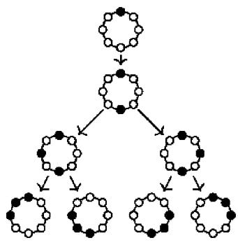
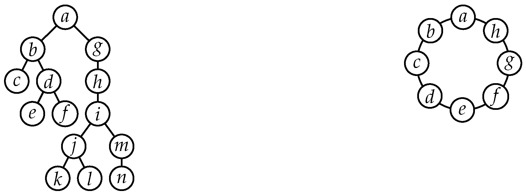
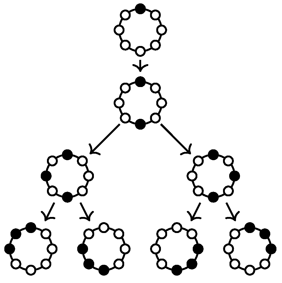
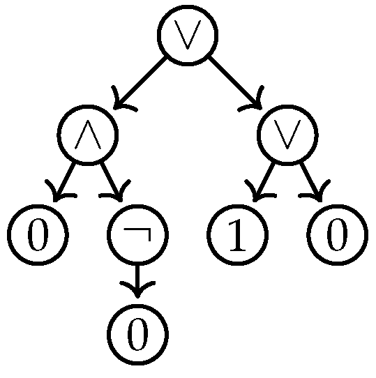
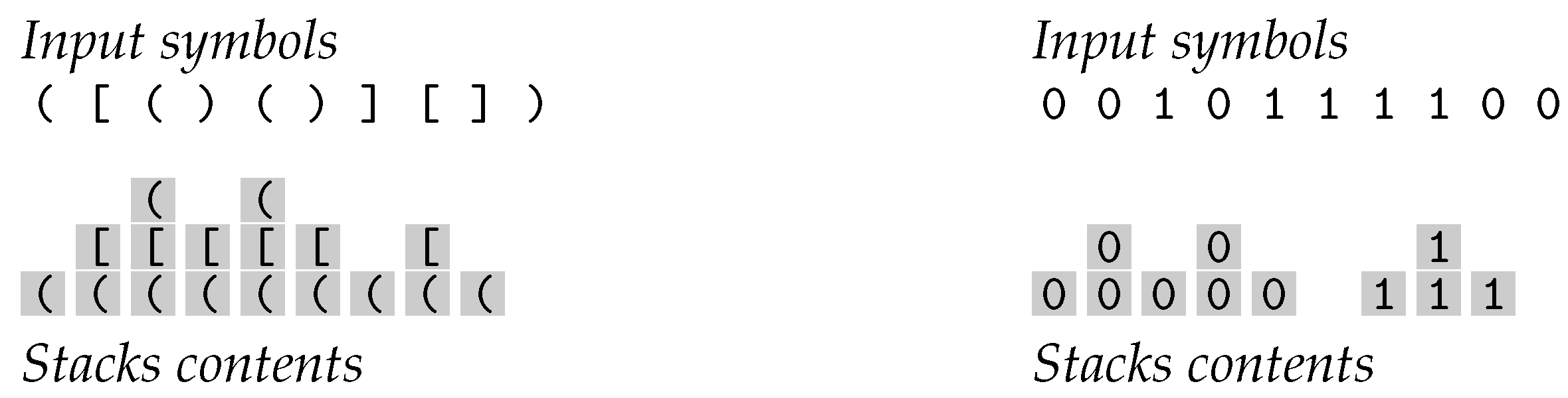
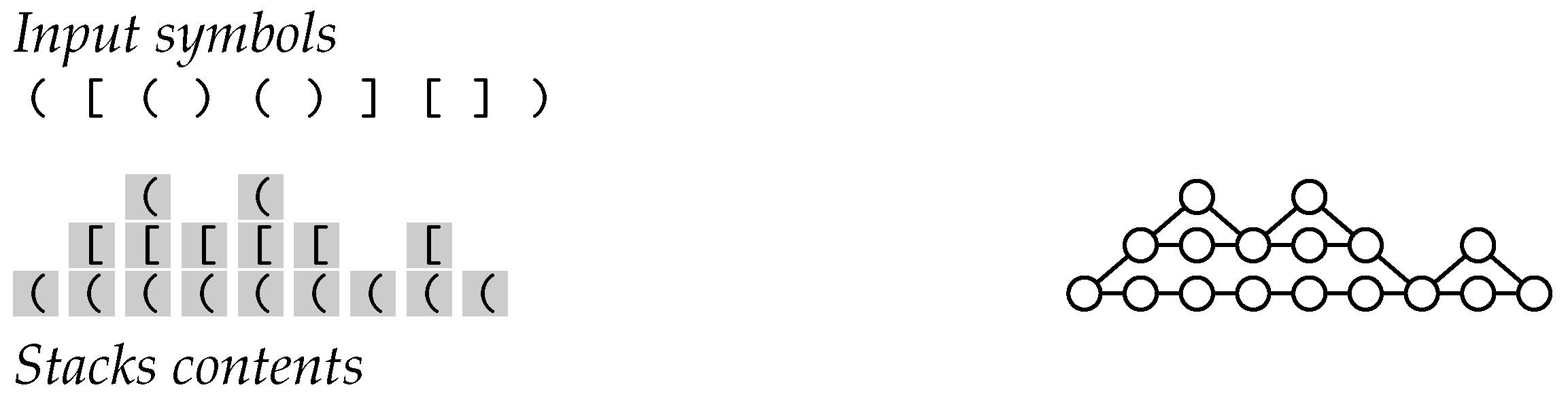
 , the black vertices form the only even cycle). It is not difficult to show that, just like the vertex cover problem and just like about any other interesting problem, the even cycle problem can be described in monadic second-order logic, and thus be solved efficiently on tree-like graphs. Now, what about highly interconnected graphs that are not tree-like? Do their many edges somehow help in deciding whether the graph has an even cycle? It turns out that the answer is a resounding “yes”: such graphs always have an even cycle [6]. In other words, we can solve the even cycle problem on arbitrary graphs as follows: if the input graph is not tree-like, simply answer “yes”, otherwise apply Courcelle’s Theorem to it.
 ) and to write in unary, I would need a blackboard larger than the universe. How difficult is the resulting unary-subset-sum problem? It is easy to see that the problem lies in NL (so it is already much easier than the normal version) and Cook [24] made an educated guess in 1985 that it is “a problem in NL which is probably not complete”. However, research got stuck at this point and an improvement on the NL bound was only obtained in 2010 when algorithmic metatheorems became available that apply to logarithmic space and the below:
 ) gets turned into the following forest of tree width 1 (note that the target number is not part of it):


