
Opposition-Based Adaptive Fireworks Algorithm

Department of Computer Information Engineering, Guangdong Technical College of Water Resource and Electrical Engineering, Guangzhou 510635, China
Algorithms 2016, 9(3), 43; https://doi.org/10.3390/a9030043
Submission received: 2 April 2016
/
Revised: 13 June 2016
/
Accepted: 4 July 2016
/
Published: 8 July 2016
(This article belongs to the Special Issue Metaheuristic Algorithms in Optimization and Applications)
Abstract
:A fireworks algorithm (FWA) is a recent swarm intelligence algorithm that is inspired by observing fireworks explosions. An adaptive fireworks algorithm (AFWA) proposes additional adaptive amplitudes to improve the performance of the enhanced fireworks algorithm (EFWA). The purpose of this paper is to add opposition-based learning (OBL) to AFWA with the goal of further boosting performance and achieving global optimization. Twelve benchmark functions are tested in use of an opposition-based adaptive fireworks algorithm (OAFWA). The final results conclude that OAFWA significantly outperformed EFWA and AFWA in terms of solution accuracy. Additionally, OAFWA was compared with a bat algorithm (BA), differential evolution (DE), self-adapting control parameters in differential evolution (jDE), a firefly algorithm (FA), and a standard particle swarm optimization 2011 (SPSO2011) algorithm. The research results indicate that OAFWA ranks the highest of the six algorithms for both solution accuracy and runtime cost.
1. Introduction
In the past twenty years several swarm intelligence algorithms, inspired by natural phenomena or social behavior, have been proposed to solve various real-world and complex global optimization problems. Observation of the behavior of ants searching for food lead to an ant colony optimization (ACO) [1] algorithm, proposed in 1992. Particle swarm optimization (PSO) [2], announced in 1995, is an algorithm that simulates the behavior of a flock of birds flying to their destination. PSO can be employed in the economic statistical design of control charts, a class of mixed discrete-continuous nonlinear problems [3] and used in solving multidimensional knapsack problems [4,5], etc. Mimicking the natural adaptations of the biological species, differential evolution (DE) [6] was published in 1997. Inspired by the behavior of the flashing characteristics of fireflies, a firefly algorithm (FA) [7] was presented in 2009, and a bat algorithm (BA) [8] was proposed in 2010 which is based on the echolocation of microbats.
The fireworks algorithm (FWA) [9] is considered a novel swarm intelligence algorithm. It was introduced in 2010 and mimics the fireworks explosion process. The FWA provides an optimized solution for searching a fireworks location. In the event of a firework randomly exploding, there are explosive and Gaussian sparks produced in addition to the initial explosion. To determine the firework’s local space, a calculation of explosive amplitude and number of explosive sparks is made based on other fireworks and fitness functions. Fireworks and sparks are then filtered based on fitness and diversity. Using repetition, FWA focuses on smaller areas for optimized solutions.
Various types of real-world optimization problems have been solved by applying FWA, such as factorization of a non-negative matrix [10], the design of digital filters [11], parameter optimization for the detection of spam [12], reconfiguration of networks [13], mass minimization of trusses [14], parameter estimation of chaotic systems [15], and scheduling of multi-satellite control resources [16].
However, there are disadvantages to the FWA approach. Although the original algorithm worked well on functions in which the optimum is located at the origin of the search space, when the optimum of origin is more distant it becomes more challenging to locate the correct solution. Thus, the quality of the results of the original FWA deteriorates severely with the increasing distance between the function optimum and the origin. Additionally, the computational cost per iteration is high for FWA compared to other optimization algorithms. For these reasons, the enhanced fireworks algorithm (EFWA) [17] was introduced to enhance FWA.
The explosion amplitude is a significant variable and affects the performance of both the FWA and EFWA. In EFWA, the amplitude is near zero with the best fireworks, thus employing an amplitude check with a minimum. An amplitude like this is calculated according to the maximum number of evaluations, which leads to a local search without adaption around the best fireworks. Thus, the adaptive fireworks algorithm (AFWA) introduced an adaptive amplitude [18] to improve the performance of EFWA. In AFWA, the adaptive amplitude is calculated from a distance between filtered sparks and the best fireworks.
AFWA improved the performance of EFWA on 25 of the 28 CEC13’s benchmark functions [18], but our in-depth experiments indicate that the solution accuracy of AFWA is lower than that of EFWA. To improve the performance of AFWA, opposition-based learning was added and used to accelerate the convergence speed and increase the solution accuracy.
Opposition-based learning (OBL) was first proposed in 2005 [19]. OBL simultaneously considers a solution and its opposite solution; the fitter one is then chosen as a candidate solution in order to accelerate convergence and improve solution accuracy. It has been used to enhance various optimization algorithms, such as differential evolution [20,21], particle swarm optimization [22], the ant colony system [23], the firefly algorithm [24], the artificial bee colony [25], and the shuffled frog leaping algorithm [26]. Inspired by these studies, OBL was added to AFWA and used to boost the performance of AFWA.
2. Opposition-Based Adaptive Fireworks Algorithm
2.1. Adaptive Fireworks Algorithm
Suppose that N denotes the quantity of fireworks, while stands for the number of dimensions, and stands for each firework in AFWA. The explosive amplitude and the number of explosion sparks can be defined according to the following expressions:
where = max(), = min(), and and are two constants. denotes the machine epsilon, ).
In addition, the number of sparks is defined by:
where and are the lower bound and upper bound of the .
Based on the above and , Algorithm 1 is performed by generating explosion sparks for as follows:
where x . U(a, b) denotes a uniform distribution between a and b.
| Algorithm 1 Generating Explosion Sparks |
| 1: for j = 1 to Si do |
| 2: for each dimension k = 1, 2, …, d do |
| 3: obtain r1 from U(0, 1) |
| 4: if r1 < 0.5 then |
| 5: obtain r from U(−1, 1) |
| 6: |
| 7: if then |
| 8: obtain r again from U(0, 1) |
| 9: |
| 10: end if |
| 11: end if |
| 12: end for |
| 13: end for |
| 14: return |
After generating explosion sparks, Algorithm 2 is performed for generating Gaussian sparks as follows:
where NG is the quantity of Gaussian sparks, m stands for the quantity of fireworks, denotes the best firework, and N(0, 1) denotes normal distribution with an average of 0 and standard deviation of 1.
| Algorithm 2 Generating Gaussian Sparks |
| 1: for j = 1 to NG do |
| 2: Randomly choose i from 1, 2, ..., m |
| 3: obtain r from N(0, 1) |
| 4: for each dimension k = 1, 2, …, d do |
| 5: |
| 6: if then |
| 7: obtain r from U(0, 1) |
| 8: |
| 9: end if |
| 10: end for |
| 11: end for |
| 12: return |
For the best sparks among the above explosion sparks and Gaussian sparks, the adaptive amplitude of fireworks in generation + 1 is defined as follows [18]:
where denotes all sparks generated in generation , denotes the best spark and x stands for fireworks in generation .
The above parameter is suggested to be a fixed value of 1.3, empirically.
Algorithm 3 demonstrates the complete version of the AFWA.
| Algorithm 3 Pseudo-Code of AFWA |
| 1: randomly choosing m fireworks |
| 2: assess their fitness |
| 3: repeat |
| 4: obtain Ai (except for A*) based on Equation (1) |
| 5: obtain Si based on Equations (2) and (3) |
| 6: produce explosion sparks based on Algorithm 1 |
| 7: produce Gaussian sparks based on Algorithm 2 |
| 8: assess all sparks’ fitness |
| 9: obtain A* based on Equation (4) |
| 10: retain the best spark as a firework |
| 11: randomly select other m − 1 fireworks |
| 12: until termination condition is satisfied |
| 13: return the best fitness and a firework location |
2.2. Opposition-Based Learning
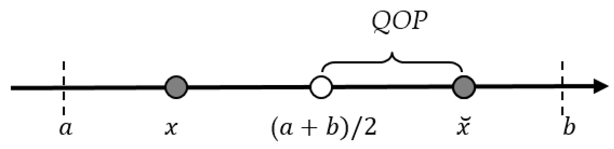
Definition 1.
Assume P = (x1, x2, ..., xn) is a solution in n-dimensional space, where x1, x2, …, xn R and xi [, ], i {1, 2, …, n}. The opposite solution OP = (, , …, ) is defined as follows [19]:
In fact, according to probability theory, 50% of the time an opposite solution is better. Therefore, based on a solution and an opposite solution, OBL has the potential to accelerate convergence and improve solution accuracy.
Definition 2.
It is proved that the quasi-opposite solution QOP is more likely than the opposite solution OP to be closer to the solution.
Figure 1 illustrates the quasi-opposite solution QOP in the one-dimensional case.
2.3. Opposition-Based Adaptive Fireworks Algorithm
The OBL is added to AFWA in two stages: opposition-based population initialization and opposition-based generation jumping [20].
2.3.1. Opposition-Based Population Initialization
In the initialization stage, both a random solution and a quasi-opposite solution QOP are considered in order to obtain fitter starting candidate solutions.
Algorithm 4 is performed for opposition-based population initialization as follows:
| Algorithm 4 Opposition-Based Population Initialization |
| 1: randomly initialize fireworks pop with a size of m |
| 2: calculate a quasi opposite fireworks Qpop based on Equation (6) |
| 3: assess 2 × m fireworks’ fitness |
| 4: return the fittest individuals from {pop ∪ Opop} as initial fireworks |
2.3.2. Opposition-Based Generation Jumping
In the second stage, the current population of AFWA is forced to jump into some new candidate solutions based on a jumping rate, Jr.
| Algorithm 5 Opposition-Based Generation Jumping |
| 1: if (rand(0, 1) < Jr) |
| 2: dynamically calculate boundaries of current m fireworks |
| 3: calculate a quasi opposite fireworks Qpop based on Equation (6) |
| 4: assess 2 × m fireworks’ fitness |
| 5: end if |
| 6: return the fittest individuals from {pop ∪ Opop} as current fireworks |
2.3.3. Opposition-Based Adaptive Fireworks Algorithm
Algorithm 6 demonstrates the complete version of the OAFWA.
| Algorithm 6 Pseudo-Code of OAFWA |
| 1: opposition-based population initialization based on Algorithm 4 |
| 2: repeat |
| 3: obtain Ai (except for A*) based on Equation (1) |
| 4: obtain Si based on Equations (2) and (3) |
| 5: produce explosion sparks based on Algorithm 1 |
| 6: produce Gaussian sparks based on Algorithm 2 |
| 7: assess all sparks’ fitness |
| 8: obtain A* based on Equation (4) |
| 9: retain the best spark as a firework |
| 10: randomly select other m – 1 fireworks |
| 11: opposition-based generation jumping based on Algorithm 5 |
| 12: until termination condition is satisfied |
| 13: return the best fitness and a firework location |
3. Benchmark Functions and Implementation
3.1. Benchmark Functions
In order to assess the performances of OAFWA, twelve standardized benchmark functions [27] are employed. The functions are uni-modal and multi-modal. The global minimum is zero.
Table 1 presents a list of uni-modal (F1~F6) and multi-modal (F7~F12) functions and their features.
3.2. Success Criterion
We utilize the success rates to compare performances of different FWA based algorithms including EFWA, AFWA, and OAFWA.
can be defined as follows:
where is the number of trials that were successful, and stands for the total number of trials. When an experiment locates a solution that is close in range to the global optimum, it is found to be a success. A successful trial is defined by:
where D denotes the dimensions of the test function, and denotes the dimension of the best result by the algorithm.
3.3. Initialization
We tested the benchmark functions using 100 independent algorithms based on various FWA based algorithms. In order to fully evaluate the performance of OAFWA, statistical measures were used including the worst, best, median, and mean objective values. Standard deviations were also determined.
In FWA based algorithms, m = 4, = 100, Me = 20, = 8, = 13, NG = 2 (population size is equivalent to 40), and Jr = 0.4. Evaluation times from 65,000 to 200,000 were used for different functions.
Finally, we used Matlab 7.0 (The MathWorks Inc., Natick, MA, USA) software on a notebook PC with a 2.3 GHZ CPU (Intel Core i3-2350, Intel Corporation, Santa Clara, CA, USA) and 4GB RAM, and Windows 7 (64 bit, Microsoft Corporation, Redmond, WA, USA).
4. Simulation Studies and Discussions
4.1. Comparison with FWA-Based Algorithms
To assess the performance of OAFWA, OAFWA is compared with AFWA, and then with FWA-based algorithms including EFWA and AFWA.
4.1.1. Comparison with AFWA
To compare the performances of OAFWA and AFWA, both algorithms were tested on twelve benchmark functions.
Table 2 shows the statistical results for OAFWA. Table 3 shows the statistical results for AFWA. Table 4 shows the comparison of OAFWA and AFWA for solution accuracy from Table 2 and Table 3.
The statistical results from Table 2, Table 3 and Table 4 indicate that the accuracy of the best solution and the mean solution for OAFWA were improved by average values of 10−288 and 10−53, respectively, as compared to AFWA. Thus, OAFWA can increase the performance of AFWA and achieve a significantly more accurate solution.
To evaluate whether the OAFWA results were significantly different from those of the AFWA, the OAFWA mean results during iteration for each benchmark function were compared with those of the AFWA. The Wilcoxon signed-rank test, which is a safe and robust, non-parametric test for pairwise statistical comparisons [28], was utilized at the 5% level to detect significant differences between these pairwise samples for each benchmark function.
The signrank function in Matlab 7.0 was used to run the Wilcoxon signed-rank test, as shown in Table 5.
Here P is the p-value under test and H is the result of the hypothesis test. A value of H = 1 indicates the rejection of the null hypothesis at the 5% significance level.
Table 5 indicates that OAFWA showed a large improvement over AFWA.
4.1.2. Comparison with FWA-Based Algorithms
To compare performances of OAFWA, AFWA, and EFWA, EFWA was tested for twelve benchmark functions. Success rates and mean error ranks for three FWA based algorithms were obtained.
Table 6 shows the statistical results for EFWA.
Table 7 compares three FWA-based algorithms.
The results from Table 6 and Table 7 indicate that the mean error of AFWA is larger than that of EFWA. The Sr of AFWA is lower that of EFWA. Thus, AFWA is not better than EFWA; The Sr of OAFWA is the highest and OAFWA ranks the highest among three FWA algorithms. Thus, OAFWA greatly improved the performance of AFWA.
For the runtimes of EFWA, AFWA and OAFWA, Table 2 and Table 3 indicate that the time cost of OAFWA is not much different from that of AFWA. But Table 2 and Table 6 indicate the time cost of OAFWA drops significantly as compared with that of EFWA.
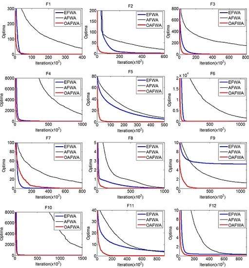
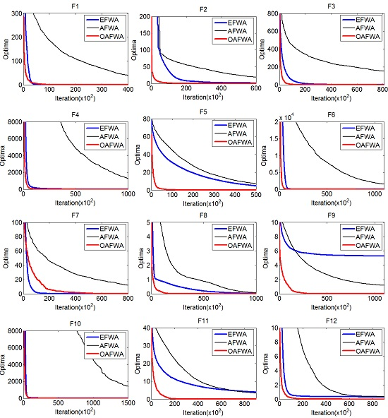
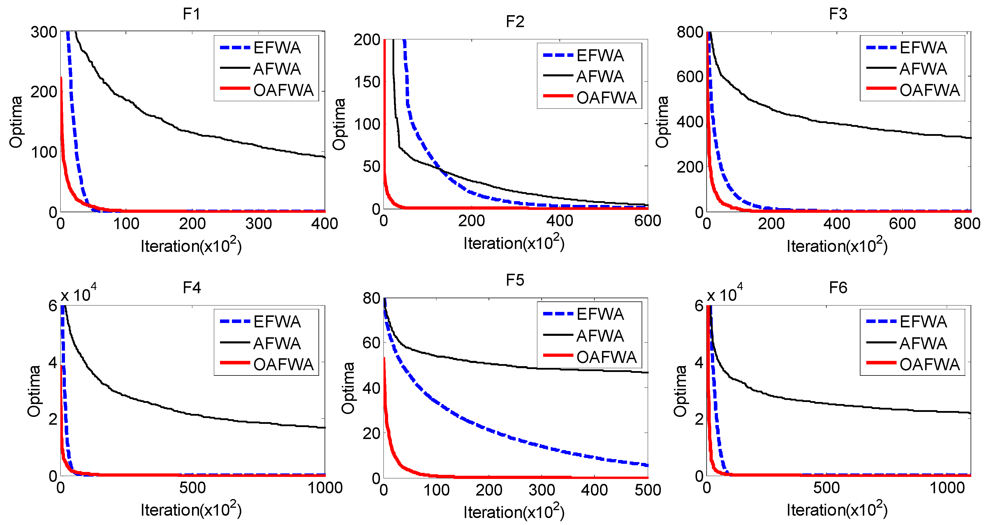
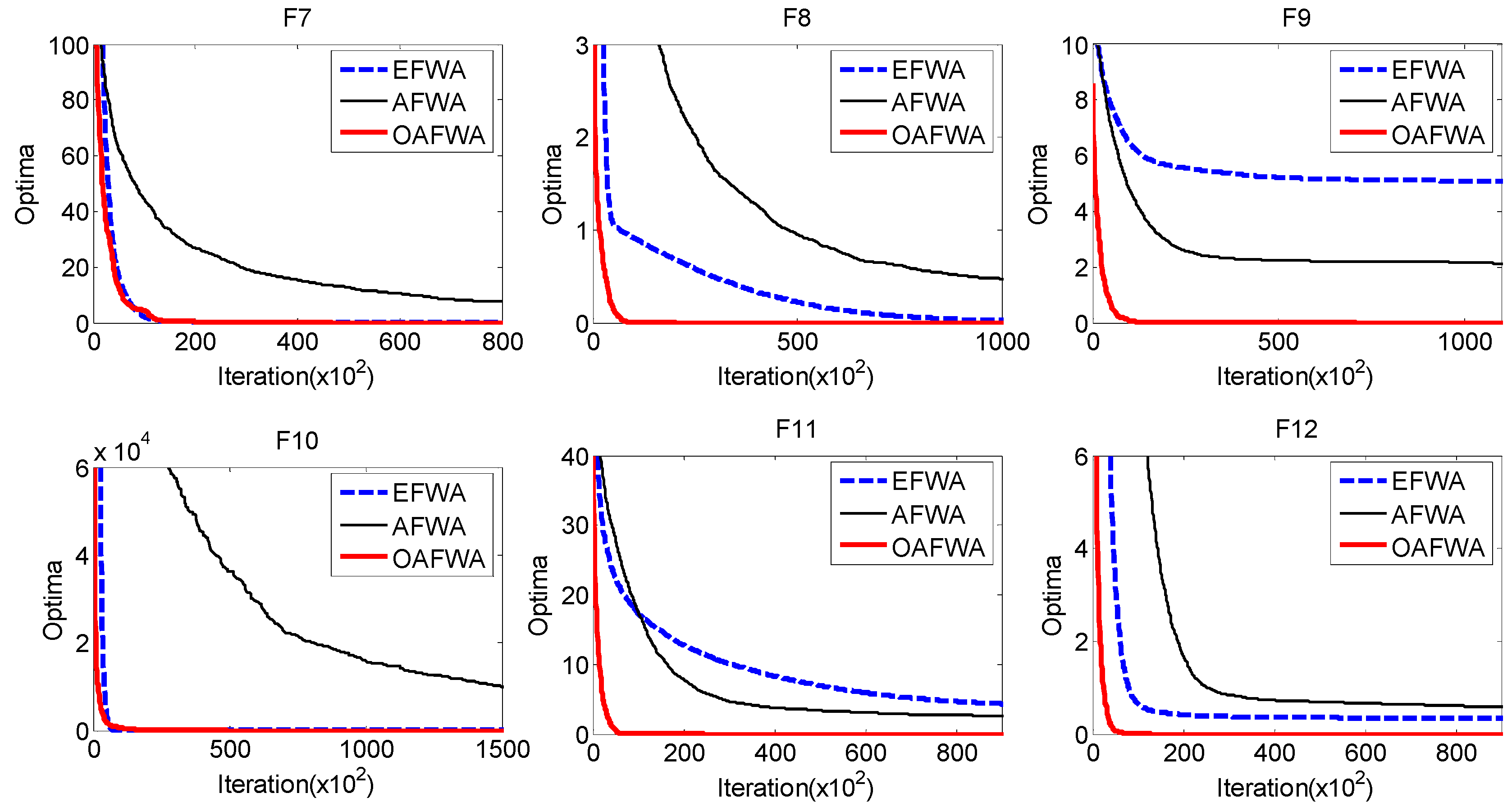
Figure 2 shows searching curves for EFWA, AFWA, and OAFWA.
Figure 2 shows that OAFWA results in a global optimum for all twelve functions and with fast convergence. However, the alternative EFWA methods do not always locate the global optimum solutions. These include EFWA for F9 and F11. AFWA is the worst among the three algorithms. It is bad for a majority of functions. Thus, OAFWA is the best one in terms of solution accuracy.
4.2. Comparison with Other Swarm Intelligence Algorithms
Additionally, OAFWA was compared with alternative swarm intelligent algorithms, including BA, DE, self-adapting control parameters in differential evolution (jDE) [29], FA, and SPSO2011 [30]. The resulting evaluation times (iteration) and population size are the same for each function. Two cases of population size are tested, 20 and 40, respectively. The parameters are shown in Table 8.
How to tune the parameters of the above algorithms is a challenging issue. These parameters are obtained from the literature [31] for BA, [29] for DE and jDE, and [30] for SPSO2011. For FA, reducing randomness increases the convergence. [32] is employed to gradually decrease . is a small constant related to iteration.
For OAFWA, m = 2, = 100, Me = 20, = 3, = 6, NG = 1 (population size is equivalent to 20), and Jr = 0.4.
Table 9 and Table 10 present the mean errors for the six algorithms when population sizes are 20 and 40, respectively.
Table 9 and Table 10 indicate that certain algorithms perform well for some functions, but less well for others. Overall, OAFWA performance was shown to have more stability than the other algorithms.
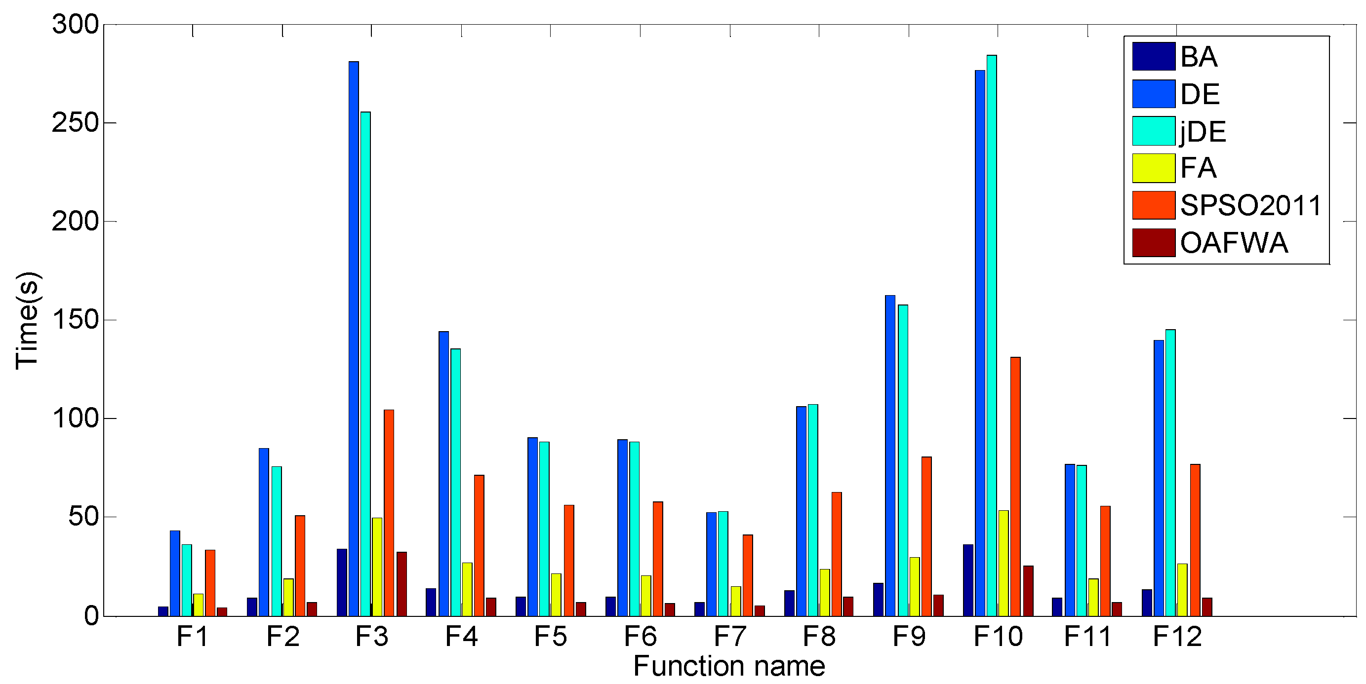
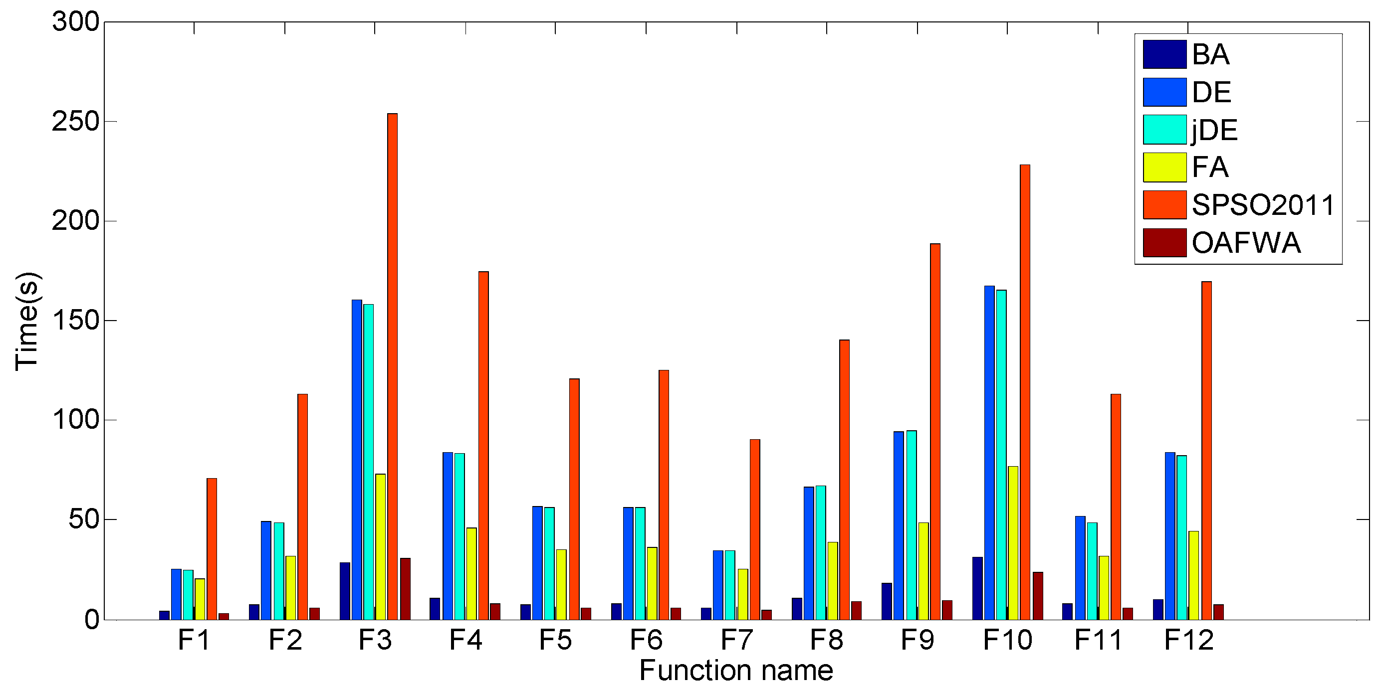
Figure 3 and Figure 4 present the runtime cost of the six algorithms for twelve functions when population sizes are 20 and 40, respectively.
Figure 3 shows that the runtime cost of DE is the most expensive among the six algorithms, except for F7, F8, F10, and F12. Figure 4 shows that the runtime cost of SPSO2011 is the most expensive among the six algorithms. The time cost of OAFWA is the least.
5. Conclusions
OAFWA was developed by applying OBL to AFWA. Twelve benchmark functions were investigated for OAFWA. Results indicated a large boost in performance in OAFWA over AFWA when using OBL. The accuracy of the best solution and the mean solution for OAFWA were improved significantly when compared to AFWA.
The experiments clearly indicate that OAFWA can perform significantly better than EFWA and AFWA in terms of solution accuracy. Additionally, OAFWA is compared with BA, DE, jDE, FA and SPSO2011. Overall, the research demonstrates that OAFWA performed the best for both solution accuracy and runtime cost.
Acknowledgments
The author is thankful to the anonymous reviewers for their valuable comments to improve the technical content and the presentation of the paper.
Conflicts of Interest
The author declares no conflict of interest.
References
- Dorigo, M. Learning and Natural Algorithms. Ph.D. Thesis, Politecnico di Milano, Milan, Italy, 1992. [Google Scholar]
- Kennedy, J.; Eberhart, R.C. Particles warm optimization. In Proceedings of the IEEE International Conference on Neural Networks, Piscataway, NJ, USA, 27 November–1 December 1995; pp. 1942–1948.
- Chih, M.C.; Yeh, L.L.; Li, F.C. Particle swarm optimization for the economic and economic statistical designs of the control chart. Appl. Soft Comput. 2011, 11, 5053–5067. [Google Scholar] [CrossRef]
- Chih, M.C.; Lin, C.J.; Chern, M.S.; Ou, T.Y. Particle swarm optimization with time-varying acceleration coefficients for the multidimensional knapsack problem. Appl. Math. Model. 2014, 38, 1338–1350. [Google Scholar] [CrossRef]
- Chih, M.C. Self-adaptive check and repair operator-based particle swarm optimization for the multidimensional knapsack problem. Appl. Soft Comput. 2015, 26, 378–389. [Google Scholar] [CrossRef]
- Storn, R.; Price, K. Differential evolution—A simple and efficient heuristic for global optimization over continuous spaces. J. Glob. Optim. 1997, 11, 341–359. [Google Scholar] [CrossRef]
- Yang, X.S. Firefly algorithms for multimodal optimization. In Proceedings of the 5th International Conference on Stochastic Algorithms: Foundation and Applications, Sapporo, Japan, 26–28 October 2009; Volume 5792, pp. 169–178.
- Yang, X.S. A new metaheuristic bat-inspired algorithm. In Nature Inspired Cooperative Strategies for Optimization (NISCO 2010); Gonzalez, J.R., Ed.; Springer: Berlin, Germany, 2010; pp. 65–74. [Google Scholar]
- Tan, Y.; Zhu, Y.C. Fireworks algorithm for optimization. In Advances in Swarm Intelligence; Springer: Berlin, Germany, 2010; pp. 355–364. [Google Scholar]
- Andreas, J.; Tan, Y. Using population based algorithms for initializing nonnegative matrix factorization. In Advances in Swarm Intelligence; Springer: Berlin, Germany, 2011; pp. 307–316. [Google Scholar]
- Gao, H.Y.; Diao, M. Cultural firework algorithm and its application for digital filters design. Int. J. Model. Identif. Control 2011, 4, 324–331. [Google Scholar] [CrossRef]
- Wen, R.; Mi, G.Y.; Tan, Y. Parameter optimization of local-concentration model for spam detection by using fireworks algorithm. In Proceedings of the 4th International Conference on Swarm Intelligence, Harbin, China, 12–15 June 2013; pp. 439–450.
- Imran, A.M.; Kowsalya, M.; Kothari, D.P. A novel integration technique for optimal network reconfiguration and distributed generation placement in power distribution networks. Int. J. Electr. Power 2014, 63, 461–472. [Google Scholar] [CrossRef]
- Nantiwat, P.; Bureerat, S. Comparative performance of meta-heuristic algorithms for mass minimisation of trusses with dynamic constraints. Adv. Eng. Softw. 2014, 75, 1–13. [Google Scholar] [CrossRef]
- Li, H.; Bai, P.; Xue, J.; Zhu, J.; Zhang, H. Parameter estimation of chaotic systems using fireworks algorithm. In Advances in Swarm Intelligence; Springer: Berlin, Germany, 2015; pp. 457–467. [Google Scholar]
- Liu, Z.B.; Feng, Z.R.; Ke, L.J. Fireworks algorithm for the multi-satellite control. In Proceedings of the 2015 IEEE Congress on Evolutionary Computation, Sendai, Japan, 25–28 May 2015; pp. 1280–1286.
- Zheng, S.Q.; Janecek, A.; Tan, Y. Enhanced fireworks algorithm. In Proceedings of the 2013 IEEE Congress on Evolutionary Computation, Cancun, Mexico, 20–23 June 2013; pp. 2069–2077.
- Li, J.Z.; Zheng, S.Q.; Tan, Y. Adaptive fireworks algorithm. In Proceedings of the 2014 IEEE Congress on Evolutionary Computation, Beijing, China, 6–11 July 2014; pp. 3214–3221.
- Tizhoosh, H.R. Opposition-Based Learning: A New Scheme for Machine Intelligence. In Proceedings of the 2005 International Conference on Computational Intelligence for Modeling, Control and Automation, Vienna, Austria, 28–30 November 2005; pp. 695–701.
- Rahnamayan, S.; Tizhoosh, H.R.; Salama, M.M. Opposition-based differential evolution algorithms. In Proceedings of the 2006 IEEE Congress on Evolutionary Computation, Vancouver, BC, Canada, 16–21 July 2006; pp. 7363–7370.
- Rahnamayan, S.; Tizhoosh, H.R.; Salama, M.M. Quasi-oppositional differential evolution. In Proceedings of the 2007 IEEE Congress on Evolutionary Computation, Singapore, 25–28 September 2007; pp. 2229–2236.
- Wang, H.; Liu, Y.; Zeng, S.Y.; Li, H.; Li, C.H. Opposition-based particle swarm algorithm with Cauchy mutation. In Proceedings of the 2007 IEEE Congress on Evolutionary Computation, Singapore, 25–28 September 2007; pp. 4750–4756.
- Malisia, A.R.; Tizhoosh, H.R. Applying opposition-based ideas to the ant colony system. In Proceedings of the 2007 IEEE Swarm Intelligence Symposium, Honolulu, HI, USA, 1–5 April 2007; pp. 182–189.
- Yu, S.H.; Zhu, S.L.; Ma, Y. Enhancing firefly algorithm using generalized opposition-based learning. Computing 2015, 97, 741–754. [Google Scholar] [CrossRef]
- Zhao, J.; Lv, L.; Sun, H. Artificial bee colony using opposition-based learning. In Advances in Intelligent Systems and Computing; Springer: Cham, Switzerland, 2015; Volume 329, pp. 3–10. [Google Scholar]
- Morteza, A.A.; Hosein, A.R. Opposition-based learning in shuffled frog leaping: An application for parameter identification. Inf. Sci. 2015, 291, 19–42. [Google Scholar]
- Mitic, M.; Miljkovic, Z. Chaotic fruit fly optimization algorithm. Knowl. Based Syst. 2015, 89, 446–458. [Google Scholar]
- Derrac, J.; Garcia, S.; Molina, D.; Herrera, F. A practical tutorial on the use of nonparametric statistical tests as a methodology for comparing evolutionary and swarm intelligence algorithms. Swarm Evol. Comput. 2011, 1, 3–18. [Google Scholar] [CrossRef]
- Brest, J.; Greiner, S.; Boskovic, B.; Mernik, M.; Zumer, V. Self-adapting control parameters in differential evolution: A comparative study on numerical benchmark problems. IEEE Trans. Evolut. Comput. 2006, 6, 646–657. [Google Scholar]
- Zambrano, M.; Bigiarini, M.; Rojas, R. Standard particle swarm optimization 2011 at CEC-2013: A baseline for future PSO improvements. In Proceedings of the 2013 IEEE Congress on Evolutionary Computation (CEC), Cancun, Mexico, 20–23 June 2013; pp. 2337–2344.
- Selim, Y.; Ecir, U.K. A new modification approach on bat algorithm for solving optimization problems. Appl. Soft Comput. 2015, 28, 259–275. [Google Scholar]
- Yang, X.S. Nature-Inspired Metaheuristic Algorithms, 2nd ed.; Luniver Press: Frome, UK, 2010; pp. 81–96. [Google Scholar]
Figure 1.
The quasi-opposite solution QOP.

Figure 2.
The EFWA, AFWA, and OAFWA searching curves.


Figure 3.
Runtime cost of the six algorithms for twelve functions when popSize = 20.

Figure 4.
Runtime cost of the six algorithms for twelve functions when popSize = 40.


| Function | Dimension | Range |
|---|---|---|
| 40 | [−10, 10] | |
| 40 | [−10, 10] | |
| 40 | [−10, 10] | |
| 40 | [−30, 30] | |
| 40 | [−100, 100] | |
| 40 | [−100, 100] | |
| 40 | [−1, 1] | |
| 40 | [−100, 100] | |
| 40 | [−10, 10] | |
| 40 | [−10, 10] | |
| 40 | [−10, 10] | |
| 40 | [−10, 10] |
| Func. | Best | Mean | Median | Worst | Std. Dev. | Time (s) |
|---|---|---|---|---|---|---|
| F1 | <1 × 10−315 | 2.46 × 10⁻³⁴ | 1.91 × 10⁻³⁴ | 1.15 × 10⁻³³ | 2.14 × 10⁻³⁴ | 3.23 |
| F2 | <1 × 10−315 | 8.21 × 10⁻¹⁷ | 3.26 × 10⁻²³ | 5.31 × 10⁻¹⁶ | 1.22 × 10⁻¹⁶ | 5.91 |
| F3 | <1 × 10−315 | 3.56 × 10−38 | 1.95 × 10−38 | 2.74 × 10−37 | 5.32 × 10−38 | 30.56 |
| F4 | <1 × 10−315 | 3.28 × 10−38 | 2.52 × 10−42 | 1.94 × 10−37 | 4.66 × 10−38 | 7.63 |
| F5 | <1 × 10−315 | 7.39 × 10⁻¹⁷ | 8.07 × 10⁻¹⁷ | 1.75 × 10⁻¹⁶ | 4.24 × 10⁻¹⁷ | 5.88 |
| F6 | <1 × 10−315 | 7.17 × 10−46 | 8.21 × 10−47 | 3.18 × 10−44 | 3.24 × 10−45 | 5.54 |
| F7 | <1 × 10−315 | 1.03 × 10⁻¹² | <1 × 10−315 | 1.02 × 10⁻¹⁰ | 1.02 × 10⁻¹¹ | 4.62 |
| F8 | <1 × 10−315 | <1 × 10−315 | <1 × 10−315 | <1 × 10−315 | <1 × 10−315 | 8.73 |
| F9 | 8.88 × 10⁻¹⁶ | 9.59 × 10⁻¹⁶ | 8.88 × 10⁻¹⁶ | 4.44 × 10⁻¹⁵ | 5.00 × 10⁻¹⁶ | 9.61 |
| F10 | <1 × 10−315 | 2.00 × 10−40 | <1 × 10−315 | 2.15 × 10−39 | 4.11 × 10−40 | 23.63 |
| F11 | <1 × 10−315 | 5.27 × 10⁻¹⁷ | 5.32 × 10⁻¹⁷ | 1.06 × 10⁻¹⁶ | 2.71 × 10⁻¹⁷ | 5.84 |
| F12 | <1 × 10−315 | 1.32 × 10⁻³³ | 1.15 × 10⁻³³ | 5.11 × 10⁻³³ | 1.00 × 10⁻³³ | 7.40 |
| Func. | Best | Mean | Median | Worst | Std. Dev. | Time (s) |
|---|---|---|---|---|---|---|
| F1 | 1.36 × 10⁻⁷ | 64.4 | 63.4 | 1.57 × 10² | 36.6 | 3.23 |
| F2 | 1.25 × 10⁻³ | 1.07 | 2.43 × 10⁻¹ | 38.9 | 3.95 | 5.59 |
| F3 | 6.45 × 10 | 2.45 × 10² | 2.49 × 10² | 4.11 × 10² | 88.2 | 30.20 |
| F4 | 4.42 × 10³ | 1.48 × 10⁴ | 1.42 × 10⁴ | 2.54 × 10⁴ | 4.84 × 10³ | 7.50 |
| F5 | 31.0 | 43.7 | 44.2 | 52.2 | 4.86 | 5.69 |
| F6 | 1.06 × 10⁴ | 2.19 × 10⁴ | 2.19 × 10⁴ | 3.18 × 10⁴ | 3.69 × 10³ | 5.38 |
| F7 | 1.51 × 10⁻⁵ | 7.66 | 5.32 | 31.8 | 7.37 | 4.54 |
| F8 | 2.20 × 10⁻¹⁰ | 3.88 × 10⁻¹ | 9.86 × 10⁻³ | 4.68 | 7.42 × 10⁻¹ | 8.28 |
| F9 | 5.51 × 10⁻⁷ | 2.11 | 2.17 | 3.57 | 6.35 × 10⁻¹ | 9.39 |
| F10 | 7.40 × 10² | 6.75 × 10³ | 6.28 × 10³ | 2.29 × 10⁴ | 4.43 × 10³ | 23.35 |
| F11 | 2.11 × 10⁻¹ | 2.39 | 1.98 | 6.69 | 1.56 | 5.64 |
| F12 | 2.00 × 10⁻¹ | 5.58 × 10⁻¹ | 5.00 × 10⁻¹ | 1.10 | 1.85 × 10⁻¹ | 7.17 |
| Func. | Best | Accuracy Improved | Mean | Accuracy Improved | ||
|---|---|---|---|---|---|---|
| AFWA | OAFWA | AFWA | OAFWA | |||
| F1 | 1.36 × 10⁻⁷ | <1 × 10−315 | −308 | 64.4 | 2.46 × 10⁻³⁴ | −35 |
| F2 | 1.25 × 10⁻³ | <1 × 10−315 | −312 | 1.07 | 8.21 × 10⁻¹⁷ | −17 |
| F3 | 64.5 | <1 × 10−315 | −316 | 2.45 × 10² | 3.56 × 10−38 | −40 |
| F4 | 4.42 × 10³ | <1 × 10−315 | −318 | 1.48 × 10⁴ | 3.28 × 10−38 | −42 |
| F5 | 31.0 | <1 × 10−315 | −316 | 43.7 | 7.39 × 10⁻¹⁷ | −18 |
| F6 | 1.06 × 10⁴ | <1 × 10−315 | −319 | 2.19 × 10⁴ | 7.17 × 10−46 | −50 |
| F7 | 1.51 × 10⁻⁵ | <1 × 10−315 | −310 | 7.66 | 1.03 × 10⁻¹² | −12 |
| F8 | 2.20 × 10⁻¹⁰ | <1 × 10−315 | −305 | 3.88 × 10⁻¹ | <1 × 10−315 | −314 |
| F9 | 5.51 × 10⁻⁷ | 8.88 × 10⁻¹⁶ | −9 | 2.11 | 9.59 × 10⁻¹⁶ | −16 |
| F10 | 7.40 × 10² | <1 × 10−315 | −317 | 6.75 × 10³ | 2.00 × 10−40 | −43 |
| F11 | 2.11 × 10⁻¹ | <1 × 10−315 | −314 | 2.39 | 5.27 × 10⁻¹⁷ | −17 |
| F12 | 2.00 × 10⁻¹ | <1 × 10−315 | −314 | 5.58 × 10⁻¹ | 1.32 × 10⁻³³ | −32 |
| Average | −288 | −53 | ||||
| F1 | F2 | F3 | F4 | F5 | F6 | |
| H | 1 | 1 | 1 | 1 | 1 | 1 |
| P | 4.14 × 10−108 | 3.33 × 10−165 | <1 × 10−315 | 2.01 × 10−230 | 1.63 × 10−181 | 1.63 × 10−181 |
| F7 | F8 | F9 | F10 | F11 | F12 | |
| H | 1 | 1 | 1 | 1 | 1 | 1 |
| P | 1.39 × 10−132 | 8.13 × 10−198 | 1.01 × 10−246 | <1 × 10−315 | 3.33 × 10−165 | 2.01 × 10−230 |
| Func. | Best | Mean | Median | Worst | Std. dev. | Time (s) |
|---|---|---|---|---|---|---|
| F1 | 1.66 × 10⁻³ | 2.63 × 10⁻³ | 2.63 × 10⁻³ | 3.44 × 10⁻³ | 3.83 × 10⁻⁴ | 4.34 |
| F2 | 2.07 × 10⁻¹ | 5.67 × 10⁻¹ | 2.75 × 10⁻¹ | 2.84 | 5.89 × 10⁻¹ | 8.88 |
| F3 | 7.52 × 10⁻³ | 1.44 × 10⁻² | 1.40 × 10⁻² | 2.77 × 10⁻² | 3.67 × 10⁻³ | 42.54 |
| F4 | 3.31 × 10⁻¹ | 5.22 × 10⁻¹ | 4.92 × 10⁻¹ | 8.91 × 10⁻¹ | 1.23 × 10⁻¹ | 13.55 |
| F5 | 1.62 × 10⁻¹ | 7.01 × 10⁻¹ | 2.18 × 10⁻¹ | 9.26 | 1.47 | 9.22 |
| F6 | 2.01 × 10⁻¹ | 3.28 × 10⁻¹ | 3.12 × 10⁻¹ | 4.75 × 10⁻¹ | 6.67 × 10⁻² | 9.11 |
| F7 | 3.22 × 10⁻³ | 5.04 × 10⁻³ | 5.07 × 10⁻³ | 6.87 × 10⁻³ | 6.73 × 10⁻⁴ | 6.46 |
| F8 | 6.01 × 10⁻³ | 1.63 × 10⁻² | 1.48 × 10⁻² | 4.91 × 10⁻² | 8.80 × 10⁻³ | 12.90 |
| F9 | 2.39 | 5.05 | 5.08 | 8.51 | 1.20 | 16.82 |
| F10 | 1.68 × 10⁻¹ | 2.69 × 10⁻¹ | 2.64 × 10⁻¹ | 4.57 × 10⁻¹ | 5.86 × 10⁻² | 37.31 |
| F11 | 9.73 × 10⁻¹ | 4.14 | 3.80 | 13.6 | 2.16 | 8.98 |
| F12 | 2.00 × 10⁻¹ | 3.15 × 10⁻¹ | 3.00 × 10⁻¹ | 4.00 × 10⁻¹ | 5.39 × 10⁻² | 13.46 |
| Func. | EFWA | AFWA | OAFWA | ||||||
|---|---|---|---|---|---|---|---|---|---|
| Mean Error | Sr | Rank | Mean Error | Sr | Rank | Mean Error | Sr | Rank | |
| F1 | 2.63 × 10⁻³ | 2 | 2 | 64.4 | 1 | 3 | 2.46 × 10⁻³⁴ | 100 | 1 |
| F2 | 5.67 × 10⁻¹ | 2 | 2 | 1.07 | 31 | 3 | 8.21 × 10⁻¹⁷ | 100 | 1 |
| F3 | 1.44 × 10⁻² | 0 | 2 | 2.45 × 10² | 6 | 3 | 3.56 × 10−38 | 100 | 1 |
| F4 | 5.22 × 10⁻¹ | 0 | 2 | 1.48 × 10⁴ | 0 | 3 | 3.28 × 10−38 | 100 | 1 |
| F5 | 7.01 × 10⁻¹ | 0 | 2 | 43.7 | 0 | 3 | 7.39 × 10⁻¹⁷ | 100 | 1 |
| F6 | 3.28 × 10⁻¹ | 0 | 2 | 2.19 × 10⁴ | 0 | 3 | 7.17 × 10−46 | 100 | 1 |
| F7 | 5.04 × 10⁻³ | 100 | 2 | 7.66 | 0 | 3 | 1.03 × 10⁻¹² | 100 | 1 |
| F8 | 1.63 × 10⁻² | 0 | 2 | 3.88 × 10⁻¹ | 0 | 3 | <1 × 10−315 | 100 | 1 |
| F9 | 5.05 | 0 | 3 | 2.11 | 0 | 2 | 9.59 × 10⁻¹⁶ | 100 | 1 |
| F10 | 2.69 × 10⁻¹ | 0 | 2 | 6.75 × 10³ | 0 | 3 | 2.00 × 10−40 | 100 | 1 |
| F11 | 4.14 | 0 | 3 | 2.39 | 0 | 2 | 5.27 × 10⁻¹⁷ | 100 | 1 |
| F12 | 3.15 × 10⁻¹ | 0 | 2 | 5.58 × 10⁻¹ | 0 | 3 | 1.32 × 10⁻³³ | 100 | 1 |
| Average | 8.7 | 2.17 | 3.2 | 2.83 | 100 | 1 | |||
| Algorithms | Parameters |
|---|---|
| BA | A = 0.95, r = 0.8, fmin = 0, f = 1.0 |
| DE | F = 0.5, CR = 0.9 |
| jDE | = 0.1, F [0.1, 1.0], CR [0, 1] |
| FA | = 0.9, = 0.25, = 1.0 |
| SPSO2011 | w = 0.7213, c1 = 1.1931, c2 = 1.1931 |
| Func. | BA | DE | jDE | FA | SPSO2011 | OAFWA | Iteration |
|---|---|---|---|---|---|---|---|
| F1 | 3.27 × 10⁻³ | 11.7 | 3.67 × 10⁻³⁵ | 6.45 × 10⁻⁷ | 8.15 × 10⁻²³ | 6.75 × 10⁻²³ | 65,000 |
| F2 | 30.4 | 3.37 | 3.49 × 10⁻³⁵ | 4.37 × 10⁻² | 6.27 | 2.02 × 10⁻¹⁶ | 100,000 |
| F3 | 2.10 × 10⁻² | 7.70 | 5.42 × 10⁻⁴ | 34.8 | 3.70 × 10⁻⁶ | 1.19 × 10−38 | 190,000 |
| F4 | 1.53 × 10⁻¹ | 2.27 × 10³ | 5.48 × 10−76 | 1.19 × 10⁻³ | 8.57 × 10⁻⁴ | 2.26 × 10−38 | 140,000 |
| F5 | 32.3 | 40.5 | 27.1 | 2.28 × 10⁻² | 12.8 | 2.22 × 10⁻¹⁷ | 110,000 |
| F6 | 1.23 × 10⁵ | 3.80 × 10³ | 2.54 × 10−58 | 7.37 × 10⁻⁵ | 9.85 × 10³ | 3.56 × 10−42 | 110,000 |
| F7 | 18.9 | 34.3 | 12.8 | 19.8 | 48.5 | <1 × 10−315 | 80,000 |
| F8 | 1.22 | 1.07 | 9.30 × 10⁻³ | 1.78 × 10⁻³ | 8.13 × 10⁻³ | 2.41 × 10⁻¹⁶ | 120,000 |
| F9 | 6.64 | 4.48 | 5.29 × 10⁻² | 3.82 × 10⁻⁴ | 2.71 | 3.40 × 10⁻¹² | 150,000 |
| F10 | 4.82 × 10⁻¹ | 5.21 × 10³ | 2.06 × 10−45 | 1.69 × 10⁻² | 3.23 × 10⁻³ | 1.17 × 10−40 | 200,000 |
| F11 | 4.85 | 6.58 × 10⁻¹ | 5.66 × 10⁻¹⁶ | 8.21 × 10⁻¹ | 3.45 | 3.03 × 10⁻¹⁷ | 100,000 |
| F12 | 16.7 | 2.41 | 1.92 × 10⁻¹ | 2.58 × 10⁻¹ | 1.92 × 10⁻¹ | 6.38 × 10⁻³⁴ | 140,000 |
| Func. | BA | DE | jDE | FA | SPSO2011 | OAFWA | Iteration |
|---|---|---|---|---|---|---|---|
| F1 | 3.22 × 10⁻³ | 7.77 × 10⁻¹⁰ | 3.27 × 10⁻¹⁷ | 2.02 × 10⁻⁵ | 4.16 × 10⁻³¹ | 2.46 × 10⁻³⁴ | 65,000 |
| F2 | 7.15 | 1.28 × 10⁻¹⁵ | 1.60 × 10⁻¹⁵ | 1.51 × 10⁻¹ | 3.06 | 8.21 × 10⁻¹⁷ | 100,000 |
| F3 | 2.03 × 10⁻² | 3.83 × 10⁻⁵ | 7.91 × 10⁻² | 40.2 | 3.25 × 10⁻⁸ | 3.56 × 10−38 | 190,000 |
| F4 | 1.23 × 10⁻¹ | 5.12 × 10⁻²² | 1.38 × 10−37 | 1.29 × 10⁻¹ | 5.77 × 10⁻⁶ | 3.28 × 10−38 | 140,000 |
| F5 | 25.1 | 23.9 | 7.27 | 9.04 × 10⁻² | 5.99 | 7.39E × 10−17 | 110,000 |
| F6 | 8.05 × 10⁴ | 2.21 × 10⁻⁶ | 2.07 × 10⁻²⁸ | 2.26 × 10⁻³ | 3.56 × 10³ | 7.17E × 10−46 | 110,000 |
| F7 | 19.2 | 26.9 | 8.08 | 18.4 | 49.1 | 1.03 × 10⁻¹² | 80,000 |
| F8 | 5.25 × 10⁻¹ | 8.39 × 10⁻³ | 2.46 × 10⁻⁴ | 1.52 × 10⁻³ | 5.22 × 10⁻³ | <1 × 10−315 | 120,000 |
| F9 | 5.53 | 5.39 × 10⁻¹ | 7.99 × 10⁻¹⁵ | 3.16 × 10⁻² | 1.54 | 9.59 × 10⁻¹⁶ | 150,000 |
| F10 | 4.62 × 10⁻¹ | 2.85 × 10⁻⁶ | 1.20 × 10⁻³⁰ | 8.71 × 10⁻² | 1.41 × 10⁻³ | 2.00 × 10−40 | 200,000 |
| F11 | 3.78 | 2.56 × 10⁻¹⁵ | 1.01 × 10⁻³ | 9.77 × 10⁻¹ | 2.17 × 10⁻¹ | 5.27 × 10⁻¹⁷ | 100,000 |
| F12 | 11.1 | 1.59 × 10⁻¹ | 9.99 × 10⁻² | 2.28 × 10⁻¹ | 1.11 × 10⁻¹ | 1.32 × 10⁻³³ | 140,000 |
| Func. | F1 | F2 | F3 | F4 | F5 | F6 | F7 | F8 | F9 | F10 | F11 | F12 | Rank |
|---|---|---|---|---|---|---|---|---|---|---|---|---|---|
| BA | 5 | 6 | 4 | 5 | 5 | 6 | 3 | 6 | 6 | 5 | 6 | 5 | 5.17 |
| DE | 6 | 4 | 5 | 6 | 6 | 4 | 5 | 5 | 5 | 6 | 3 | 4 | 4.92 |
| jDE | 1 | 1 | 3 | 1 | 4 | 1 | 2 | 4 | 3 | 1 | 2 | 2 | 2.08 |
| FA | 4 | 3 | 6 | 4 | 2 | 3 | 4 | 2 | 2 | 4 | 4 | 3 | 3.41 |
| SPSO2011 | 3 | 5 | 2 | 3 | 3 | 5 | 6 | 3 | 4 | 3 | 5 | 2 | 3.67 |
| OAFWA | 2 | 2 | 1 | 2 | 1 | 2 | 1 | 1 | 1 | 2 | 1 | 1 | 1.42 |
| Func. | F1 | F2 | F3 | F4 | F5 | F6 | F7 | F8 | F9 | F10 | F11 | F12 | Rank |
|---|---|---|---|---|---|---|---|---|---|---|---|---|---|
| BA | 6 | 6 | 4 | 5 | 5 | 6 | 4 | 6 | 6 | 6 | 6 | 6 | 5.50 |
| DE | 4 | 2 | 3 | 3 | 6 | 3 | 5 | 5 | 4 | 3 | 2 | 4 | 3.67 |
| jDE | 3 | 3 | 5 | 2 | 4 | 2 | 2 | 2 | 2 | 2 | 3 | 2 | 2.67 |
| FA | 5 | 4 | 6 | 6 | 2 | 4 | 3 | 3 | 3 | 5 | 5 | 5 | 4.25 |
| SPSO2011 | 2 | 5 | 2 | 4 | 3 | 5 | 6 | 4 | 5 | 4 | 4 | 3 | 3.91 |
| OAFWA | 1 | 1 | 1 | 1 | 1 | 1 | 1 | 1 | 1 | 1 | 1 | 1 | 1.00 |
© 2016 by the author; licensee MDPI, Basel, Switzerland. This article is an open access article distributed under the terms and conditions of the Creative Commons Attribution (CC-BY) license (http://creativecommons.org/licenses/by/4.0/).
Share and Cite
MDPI and ACS Style
Gong, C. Opposition-Based Adaptive Fireworks Algorithm. Algorithms 2016, 9, 43. https://doi.org/10.3390/a9030043
AMA Style
Gong C. Opposition-Based Adaptive Fireworks Algorithm. Algorithms. 2016; 9(3):43. https://doi.org/10.3390/a9030043
Chicago/Turabian StyleGong, Chibing. 2016. "Opposition-Based Adaptive Fireworks Algorithm" Algorithms 9, no. 3: 43. https://doi.org/10.3390/a9030043
Note that from the first issue of 2016, this journal uses article numbers instead of page numbers. See further details here.