A Hybrid Course Recommendation System by Integrating Collaborative Filtering and Artificial Immune Systems

Abstract

This research proposes a two-stage user-based collaborative filtering process using an artificial immune system for the prediction of student grades, along with a filter for professor ratings in the course recommendation for college students. We test for cosine similarity and Karl Pearson (KP) correlation in affinity calculations for clustering and prediction. This research uses student information and professor information datasets of Yuan Ze University from the years 2005–2009 for the purpose of testing and training. The mean average error and confusion matrix analysis form the testing parameters. A minimum professor rating was tested to check the results, and observed that the recommendation systems herein provide highly accurate results for students with higher mean grades.

1. Introduction

With the advent of flexible curriculum systems in many colleges and universities and an ever wider variety range of courses being offered, word-of-mouth no longer suffices in providing accurate information to students regarding the courses where they may demonstrate higher aptitude and interest. There is a present need to ensure that students make the best use of available data to make better decisions regarding their course selection.

Generally, recommendation systems are of three types: collaborative filtering, association-rule based and content based. The recommendation system herein seeks to recommend courses based on a combination of factors, such as relevance of courses to students’ department, the aptitude of students measured quantitatively in the form of grades obtained in a course and a quality-control mechanism based on filtering courses with poor instructor ratings. A modified two-tiered user-based collaborative filtering recommendation system is proposed herein to consider these factors.

Implementing a user-based collaborative recommendation system would be an appropriate choice for predicting future grades. In a user-based collaborative recommendation system, for example in an e-shopping portal, recommendations for products are based on the affinity of a user to a user group. For instance, one user purchases a phone, a screen guard and a phone cover, while another user purchases a phone and a screen guard. A collaborative filtering system would recognize the relation between these users and recommend a phone cover for the second user.

In the case of user-based collaborative filtering, user clusters will be identified quantitatively, based on their ratings/scores, and prediction values will be provided to new users based on their affinity to the cluster. In the case of our course recommendation system, students getting grades will be placed in similar cluster patterns, by using an Artificial Immune System (AIS) clustering approach for calculating the affinities between different students in a training data pool. The AIS algorithm has proven to be an effective method for sorting data into clusters. The AIS technique will enhance the quality of the solution provided herein. The affinity values of new students in clusters are then used as weights in calculating the predicted values.

The knowledge a student gains and the interest developed in a subject often depends on the quality of education imparted by the instructor. We therefore test the effects of filtering out courses where the instructors scored poorly in feedback evaluation, on our prediction matrix to observe the effects on prediction accuracy.

2. Background Knowledge

2.1. Course Recommendation Systems

Farzan and Brusilovsky [1] presented CourseAgent, an adaptive community-based hypermedia system that provides course recommendations based on feedback from students’ assessment of course relevance to their career goals. Observing the progress of the students using the course recommendation system provides good information feedback regarding the system. Parameswaran et al. [2] developed a course recommendation system, CourseRank, which recommends courses that satisfy student criteria. The system includes two frameworks for course requirements, and considers the dual problems of checking requirements and making recommendations. Data mining is also used to develop the course recommendation system. Aher and Lobo [3] show that data mining techniques, such as clustering and association rule methods, are useful in course recommendation systems. They extract data based on students’ behavioral patterns and analyze the collected data by data mining techniques.

2.2. Artificial Immune System

The immunological system of vertebrates is a very complex and superior mechanism that provides defense against a vast variety of antigens. Thus it has inspired much research by scientists and engineers across various disciplines, who seek to find solutions for their problems, the same way the immunological system seeks solutions to counter pathogens. The immunity it provides is both innate (from memory) and adaptive (in dealing with new pathogens).

There are three major immunological principles applied for immune system methods: immune network theory, mechanisms of negative selection and clonal selection principles [4]. Immune network theory was first proposed by Jerne [5] in 1974. He suggested that in a real immune system, when a biological organism encounters an invasion from outside pathogens, the biological organism develops its own protective agents, antigens. Immune systems produce antibodies to combine with antigens to fight off pathogens as an immune response. This process from the immune system suggests a good approach for finding the best solution to an optimization problem [6]. The antigen would be the objective function and the antibodies, possible solutions to the problem. Dudek [7] focused on the antigen, and searched for an antibody that can combine with it to create a new solution to the problem.

In 2003, Dasgupta et al. [4] pointed out that the immune system is a complex system with strong information processing characteristics, such as feature selection, pattern recognition, learning and memory recall, and other functions. Alatas and Akin [8] used the AIS algorithm for the mining of fuzzy classification rules in order to improve classification accuracy by saving the best classification rules for each category in the database. Chong and Chen [9] advocate the use of AIS for proactive management and forecasting of dynamic customer requirements to lower the risks in developing products for quickly shifting markets. References [10,11] show the effective use of AIS for data analysis. Coello et al. [12] show the use of AIS in job shop scheduling. Aickelin and Chen [13] use the concept of AIS and affinity measures in building effective movie recommendation techniques.

2.3. Collaborative Filtering

The main objective of user-based collaborative filtering is to employ users with similar interests in recommending items. Through cooperation, the information is recorded and filtered to help obtain more accurate recommendation results for users. The information collected is not limited to that derived from people with similar interests. It is also important to collect information from people with dissimilar interests, which is known as social filtering. This is an important feature for e-commerce. This paper focuses on the customer’s past purchasing behavior and compares it to those of other group customers with similar purchasing behaviors to recommend a list of items for the target customer that he or she might like. From the group preferences, we are able to recommend products and services single persons. In recent years, different algorithms based on mathematical formulae have been applied to improve the recommendation system by determining the strength of interest and these numerical formulae establish a strong basis for collaborative filtering. Helge and Thomas [14] proposed a probabilistic collaborative filtering model and applied it to the MovieLens data. Their experimental results show that the probabilistic collaborative model can obtain implicit information about the target domain that is modeled using certain hidden variables. Jesus [15] provided a collaborative filtering method based on two aspects. One is a joint user group recommendation, while the other employs similar groups with referenced items, from joint collaborative filtering to using limited references or combining two cases to provide similar recommendations. Buhwan [16] presented a semi-explicit rating method, based on the unrated factor in a semi-supervised approach, to conduct an experiment. The experimental results show that the semi-explicit rating data are better than purely explicit rating data. Sung Ho Ha [17] used cluster analysis for customer segmentation and discovered customer segment knowledge to build a segment transition path, and then predicts customer segment behavior patterns. References [18,19,20] show the benefits of collaboration in recommender systems.

2.4. Karl Pearson Coefficient and Cosine Similarity

The two most popular measures for measuring similarities quantitatively between different users based on their ratings are the Karl Pearson (KP) coefficient and cosine similarity function and their variants. They are statistical measures of the degree of association between two vectors. Both have been applied successfully for calculating correlations in a variety of scenarios [21,22,23,24].

The Pearson correlation similarity of two users x, y is defined as:

$$simil\left(x,y\right)=\frac{{\sum }_{i\in I_{x,y}}\left(r_{x,i}- \overline{r_x}\right)\left(r_{y,i}- \overline{r_y}\right)}{\sqrt{{\sum }_{i\in I_{x,y}}{\left(r_{x,i}-\overline{r_x}\right)}^2 {\sum }_{i\in I_{x,y}}{\left(r_{y,i}-\overline{r_y}\right)}^2}}$$

(1)

where I_x,y is the set of items rated by both user x and user y. For the KP correlation, the magnitude of the value determines to what degree the users are correlated, and the sign indicates the direction of the relation. The value ranges from −1 to 1. Values near one indicate a high degree of correlation between users, signifying that the pattern of students’ grades is similar. Values near minus one indicate a high degree of negative correlation between users, so the pattern of grades would be the opposite. The courses with the crests of grades for one student would be the troughs for the other. Zero indicates that the pattern of grades of the students is hardly related.

The cosine-based approach defines the cosine-similarity between two users x and y as:

$$simil\left(x,y\right)=\cos \left(\overrightarrow{x},\overrightarrow{y}\right)= \frac{ \overrightarrow{x}·\overrightarrow{y}}{\Vert \overrightarrow{x}\Vert \times \Vert \overrightarrow{y}\Vert }=\frac{{\sum }_{i\in I_{xy}}{r}_{x,i}{r}_{y,i}}{\sqrt{{\sum }_{i\in I_x}{r}_{x,i}^2}\sqrt{{\sum }_{i\in I_y}{r}_{y,i}^2}}$$

(2)

For the cosine, if all of the vector elements are positive, as in the case of course grades, the magnitude behaves as a scalar, with high values indicating high correlation, and low values indicating high negative correlation. Values near one denote high correlation; values near zero indicate negative correlation. Less related data would have cosine values somewhere in between.

2.5. Confusion Matrix

A confusion matrix, as shown in

Table 1. Diagram illustrating the confusion matrix.

	Condition Positive	Condition Negative
Test outcome positive	True Positive	False Positive
Test outcome negative	False Negative	True Negative

, also known as a contingency table or an error matrix, is the matrix created when each column represents the predicted outcomes of a predicted class, while each row represents the occurrence of instances in an actual class. It allows for easy visualization of errors and comparisons. It derives its name from the fact that it shows the errors made by a forecasting model when it is “confused”, and is an appropriate choice as it will check for errors not just for the recommended courses but also for all instances of the test data.

In this research, two classes are used: the positive class and the negative class. Such a matrix is called a table of confusion. It is a 2-by-2 matrix that contains the instances of true positives, false positives, true negatives, and false negatives. Stephen V. Stehman [25] uses the error matrix for the accuracy assessment of land-cover maps constructed from remotely sensed data. Tom Fawcett [26] employs the confusion matrix and its derivative metrics for his guide to using receiver operating characteristic (ROC) graphs for visualizing, organizing and selecting classifiers based on their performance. Lewis and Brown [27] use a generalized confusion matrix for assessing the estimates of areas based on remotely sensed data.

3. Purposed Approaches

Most course recommendation systems focus on users’ interests and social network to find out what the users like or are interested in. Therefore, these kinds of systems mine the data from users’ personal data, social networking sites, etc. In this study, the focus is on “grades”; this means that the aim of this research is to develop a course recommendation system to help users find courses in which they can get high scores. Thus, we collected data including the courses which users learned and what scores they received. In addition, we also collected data on the teachers of the courses, such as whether or not a teacher is popular with the students. Next, we adapted these three related data as the input to the proposed classification model so that the model can provide suggestions for users to learn in which courses they can get high scores. The following offers more details on this research.

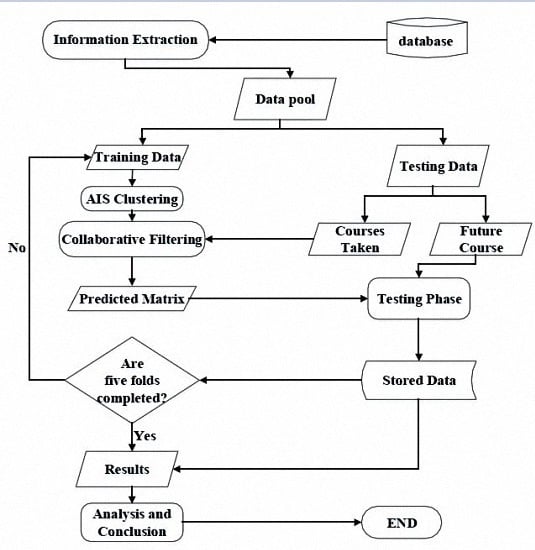
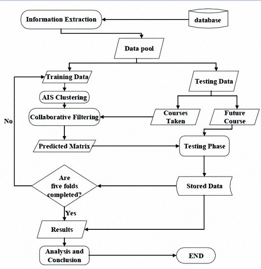
A Flow Diagram of the procedure for the design of the course recommendation system is shown in Figure 1. After the information extraction, the student course data and course grades are retrieved from the school database. Then, in the training phase, student data are defined as antigens, and weighted cosine similarity is used to assess the affinity between antigens and antibodies to find the relations between the data for clustering. In the testing phase, the collaborative filtering method is applied on the data cluster to predict the rating for the course. Analysis is done based on mean average error and the generated confusion matrix. We then make suggestions based on the students’ expected grades and the professors’ rating for the course.

3.1. Information Extraction

The data on professors and the student course data for the years 2005–2009 are provided in a tabular format as shown in

Table 2. Professor data tabular example.

Year	Professor Name	Course ID	Course Class	Average Rating
2006	Ms. XYZ	EL102	A	2.3
2006	Mr. ABC	EL102	B	1.9
2006	Ms. PQR	PO210	A	3.6

Note: A course may have one or more course classes given by the same/different professors.

and

Table 3. Student Course data tabular example.

Year of Course	Student ID	Course ID	Course Class	Student Grade	Numeric Grade	Course Grade (Year)
2006	9510036	EL102	A	A	4	1
2006	9510037	EL102	A	B	3	1
2006	9430001	PO210	H1	C	2	2
2006	9330010	PO311	B	D	1	3

. Course grade refers to the academic year in which the student is expected to select the course.

For use in a collaborative filtering model, we sorted the student grade data as a matrix, as shown in

Table 4. Student course matrix denoting grade.

Grade Matrix	EL102	PO210	PO311	AC205	OM291
9510036	4		3		3
9510037	3			4
9530001		2		3	2
9530010	2		1

. Similarly, another two cells were created containing year and course class in place of grade for professor data retrieval. There were 22,262 students who had taken at least one of the 3455 courses offered by Yuan Ze University during this time span. A major problem limiting the usefulness of collaborative filtering is the sparsity problem, which refers to a situation in which data are insufficient to identify similarities in consumer interests. As students will take fewer than sixty of the 3455 courses offered, directly applying a collaborative filter would not be efficient or accurate. Hence we use a demographic property of the student population, their department, to segregate the data. This forms the first layer of our two-layer collaborative filtering system, where we initially filter courses based on a similarity of users, a common department.

A sub matrix consisting only of students in a particular department and the courses taken by them in the six-year span is used for the data pool. Hence, it is now possible to work with a smaller but adequate set of data, which contains courses bearing relevance to the students of the department. These courses may be taken within or outside the department. A significant advantage to this method is that, while the data are centralized, we can still use the data in a decentralized manner. We can compare our recommendation system for multiple departments from the same data set with reduced computation time and high accuracy.

In the following, the development and testing of the proposed recommendation system is explicitly defined. The aim of the system is to recommend courses of years 3 and 4 for third-year undergraduate students who have taken courses of years 1 and 2. For this, a rider is established that the student should have completed a minimum of 15 courses in his/her first two years, which is both a logical step as years 3 and 4 courses must not be taken without having completed sufficient courses of years 1 and 2, as well as a practical step to avoid the cold start scenario where insufficient data would preclude computing user similarities efficiently. Thus, the number of students (rows) in the data pool whose information would have not been very useful for the collaborative procedure is further reduced.

The reduced size of the student course matrix (data pool) for the Department of Chinese Linguistics and Literature (Undergraduate Program) is 165 × 437 (165 students, 437 courses).

For the purpose of training and testing, we divide our data into five parts, four for training and one for testing cyclically. The statistical results obtained for the given data pool will be the mean of the results obtained from each fold.

3.2. Artificial Immune System

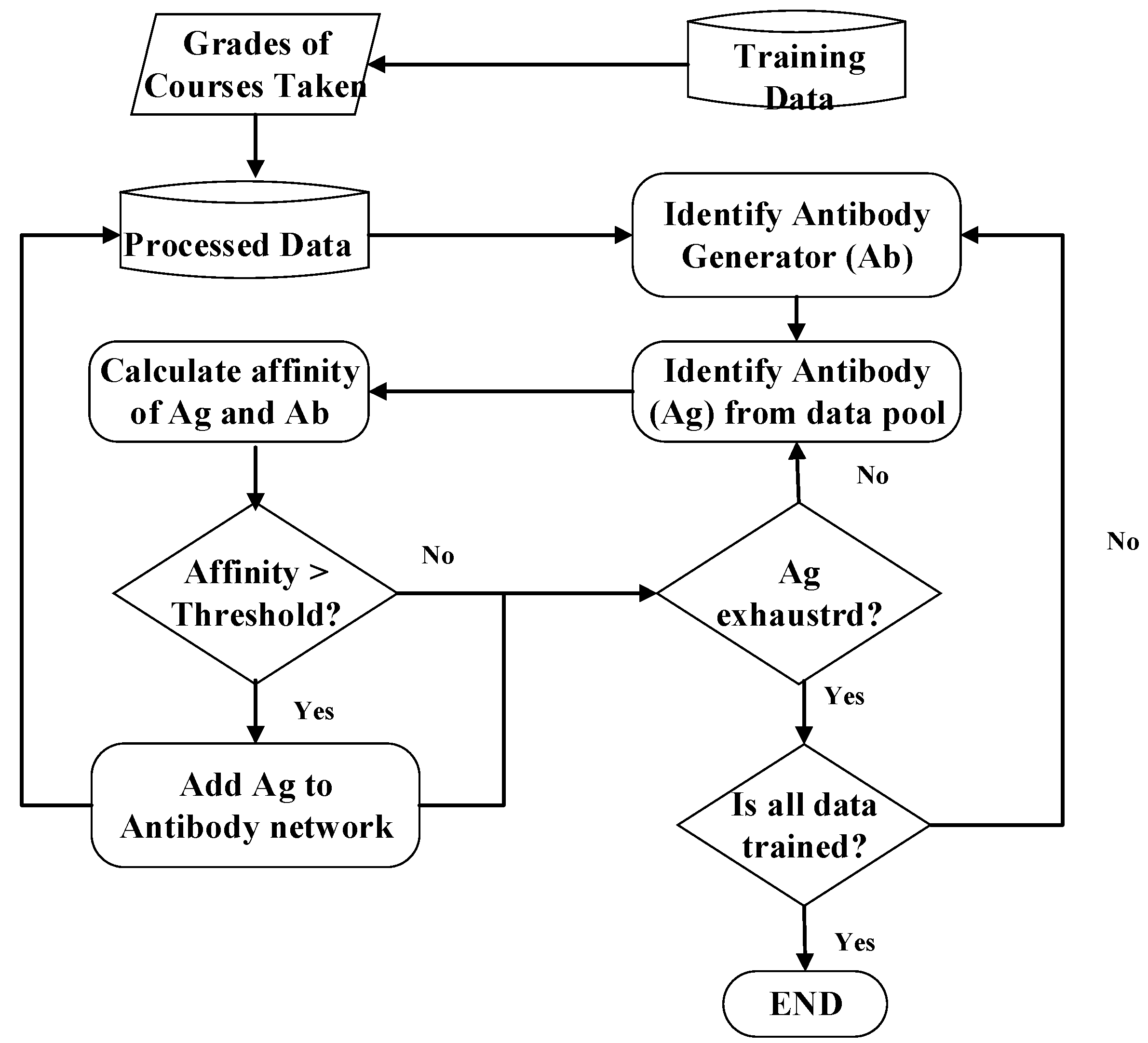
The affinity in the immune network theory was combined with the concepts of the expansion diagram for use in the clustering algorithm. The flowchart for the AIS algorithm in clustering is shown in Figure 2.

In the expansion diagram, the members of the data pool to be clustered are plotted and the distance between them is measured by the inverse of their affinity. Higher affinity between two members implies that they will be located closer together. In this research, every single datum is treated as an antigen or antibody. The expansion diagram used in AIS clustering is depicted in Figure 3.

The procedures of AIS clustering are explained in the following:

Step 1. Plot the data pool for training: These untrained data are used for both antibodies and antigens.

Step 2. Select any untrained datum randomly as an antibody generator to start creating a new antibody network.

Step 3. Identify antigens: Every datum is used as an antigen, even those who are members of another antibody network.

Step 4. Calculate affinity: When the antibodies are trying to identify the antigens, the binding between the antibody and antigen has to be determined; the stronger the binding, the closer the antigen is to the antibody.

Step 5. Identify Cluster: The antigens that are closer to the antibody generator than a pre-specified threshold are identified. If the antigen is a member of another antibody network it identifies with the one whose antibody generator is closer.

Step 6. Generate new antibodies: The antigens that have bonded with the antibody generator now form an antibody network.

Step 7. Check termination conditions: If all of the data have been trained, go to Step 8. Otherwise, go back to Step 2.

Step 8. Terminate!

In this research, every single datum is treated as an antigen or antibody. The affinity between the data is calculated for clustering. The Pseudo-Code for AIS clustering is illustrated in Pseudo-Code 1:

Pseudo-Code 1 AIS Clustering in Training Data
1:	Ab_data = student course data with courses taken from years 1 and 2 #training data
2:	Ag_data = Ab_data #every training data used as both antibody and antigen
3:	INITIALIZE: Max_Threshold = zeros(size(Ag_data)) #stores best affinity value
4:	INITIALIZE: cluster_number = zeros(size(Ag_data)) #stores antibody network No
5:	INITIALIZE: cluster = 1;
6:	FOR i = 1:size(Ab_data) #loop for all Ab
7:	IF MaxThreshold(I) < Threshold #identify untrained data as antibody
8:	cluster = cluster + 1; #find antibody network number
9:	FOR j = 1:size (Ag_data) #run loop for all Ag
10:	Affinity = Affinity_function(Ab(i),Ag(j));
11:	IF Affinity > Threshold & Affinity > Threshold_Max(i) #check for strongest bond
12:	Max Threshold(j) = Affinity; #Store best bonding value
13:	cluster_number(j) = cluster; #Store Antibody Network No
14:	END IF
15:	END FOR
16:	END IF
17:	END FOR

Those antibodies with the same cluster number create the antibody networks in the above pseudo-code. These antibody networks will be used in the collaborative filtering to match antigens (testing data) with similar user groups.

3.3. Using Karl Pearson Correlation and Cosine Similarity as Affinity Functions

As shown in

Table 5. Example for calculation demonstration.

Course	A	B	C	D	E
Student 1 (Antibody x)	3		3	5	4
Student 2 (Antigen y)	2	2		4	3

, an example of affinity is as follows:

(1)

Using the Karl Pearson Correlation

$$simil\left(x,y\right)=\frac{{\sum }_{i\in I_{x,y}}\left(r_{x,i}-\overline{r_x}\right)\left(r_{y,i}-\overline{r_y}\right)}{\sqrt{{\sum }_{i\in I_{x,y}}{\left(r_{x,i}-\overline{r_x}\right)}^2{\sum }_{i\in I_{x,y}}{\left(r_{y,i}-\overline{r_y}\right)}^2}}$$

• I_x,y = 3 (Courses A, D and E taken by same users from Table 5);
• r_x,i = numeric grade of student x in course i;
• $\overline{r_{x }}$ = (3 + 3 + 5 + 4)/4 = 3.75;
• $\overline{r_y}$ = (2 + 2 + 4 + 3)/4 = 11/3 = 3.67 = mean grade of student x;

  $$\text{KP Similarity }=\frac{\left(3-3.75\right)\left(2-3.67\right)+\left(5-3.75\right)\left(4-3.67\right)+\left(4-3.75\right)\left(3-3.67\right)}{\sqrt{\{{\left(3-3.75\right)}^2+{\left(5-3.75\right)}^2+{\left(4-3.75\right)}^2\}\left\{{\left(2-3.67\right)}^2+{\left(4-3.67\right)}^2+{\left(3-3.67\right)}^2\right\}}}=1$$

(2)

Using weighted Karl Pearson Correlation: Preference is given to students who have more courses in common with the antigen student by assigning a weight = common courses watched/total courses.

Weighted_KP_similarity = KP_similarity × I_x,y/size(Antigen) = 1 × 3/5 = 0.6

(3)

Using Cosine Similarity

$$simil\left(x,y\right)=\cos \left(\overrightarrow{x},\overrightarrow{y}\right)=\frac{\overrightarrow{x}·\overrightarrow{y}}{\Vert \overrightarrow{x}\Vert \times \Vert \overrightarrow{y}\Vert }=\frac{{\sum }_{i\in I_{x,y}}{r}_{x,i}{r}_{y,i}}{\sqrt{{\sum }_{i\in I_x}{r}_{x,i}^2}\sqrt{{\sum }_{i\in I_y}{r}_{y,i}^2}}$$

$$\text{Cosine Similarity}=\frac{3\times 2+5\times 4+4\times 3}{\sqrt{\left(3^2+3^2+5^2+4^2\right)}\sqrt{2^2+2^2+5^2+4^2)}}=0.7067$$

(4)

Using Weighted Cosine Similarity

Weighted_cosine_similarity = Cos_similarity × I_x,y/size(Antigen) = 0.7067 × 3/5 = 0.424

The data for all four equations were tested, and showed that the weighted cosine similarity provided the most accurate predictions. However, the accuracy obtained using the cosine similarity and the KP weighted similarity were close to the accuracy obtained using the weighted cosine similarity.

3.4. Collaborative Filtering

The clustered data gathered from the AIS training process are now used to predict the scores of students of the testing dataset; the results will then be compared with the actual scores. The scores the students (antigen) received in the courses in their first two years are compared with the scores received by the clustered students (antibody networks) in the trained data and the mean affinity values are calculated. The student cluster that has the highest mean affinity with the antigen student (denoted by Abtop) is used for the prediction of scores for the particular antigen via a prediction equation. This procedure is repeated for all the antigens in the testing dataset. Pseudo-Code 2 describes the pseudo-code for the collaborative filtration process.

Pseudo-Code 2 Collaborative Filtering Procedure
1:	Ag_test = testing database #contains the antigens used for testing
2:	Ab_trained = trained dataset #contains the antibody networks of trained data
3:	FOR i= 1:size(Ag_test)
4:	FOR j = 1:number of clusters
5:	Calculate the mean affinity of Ag_test(i) with cluster (j) in Ab_trained;
6:	Max_affinity = Stored value of the maximum mean affinity;
7:	Abtop = Stored cluster with maximum mean affinity;
8:	ENDFOR
9:	FOR k = 1:size(Ag_test)
10:	IF Course(k) is taken in year 3 or 4
11:	Predicted_grade = round(Prediction_equation(Ag,Abtop,k));
12:	Error = absolute difference of Ag_test(i,k) and predicted_grade;
13:	Modify the confusion matrix based on prediction vs. outcome (add one to the counter for true positive, false positive, false negative or true negative depending on the scenario);
14:	END IF
15:	END FOR
16:	END FOR

3.5. The Prediction Equation

To predict the grades of students in the courses not taken using their past data and the cluster they have maximum affinity with, the following equation is used:

$$P_{Ag,c}=\overline{R_{Ag}}+\frac{{\sum }_{Ab=1}^k{\text{Affinity}}_{Ag,Ab}\times \left(R_{Ab,c}-\overline{R_{Ab}}\right)}{{\sum }_{Ab=1}^k\left|{\text{Affinity}}_{Ag,Ab}\right|}$$

(3)

where P_Ag,c is the predicted grade of student Ag in course c, R_Ag,c is the grade of student Ag in course c, and k is the number of students in the cluster Abtop who have taken course c. The same affinity function is used in the prediction equation as was used in the AIS clustering stage. The affinity acts as a weight, such that more weight is given to the students with higher similarity to the antigen students for the prediction of their scores in a course. As the grades of students are natural numbers, the predicted value we obtain from the predicted equation is rounded off to make the results more meaningful and accurate.

4. Experimental Results

This research was undertaken by the Nature Inspired Learning and Knowledge Discovery Laboratory of the Information Management Department, Yuan Ze University (YZU), and uses the student and professor information datasets of the year 1995–1999; 22,262 students took at least one of the 3465 courses offered by YZU during this span of time. Only undergraduate students’ information was considered for the recommendation system.

The results were tabulated and tested for four recommendation scenarios.

(1)

Recommend courses where student receives Grade A or B (Numeric 4 or 3).

(2)

Recommend courses where student receives minimum Pass Grade (Grade C).

(3)

Recommend courses where student receives above average course grade.

(4)

Recommend courses where student receives above his/her average grade.

We also compared these scenarios when the minimum professor rating filter was applied. The results of these scenarios were generated using KP and cosine similarity coefficients, and compared with those where the mean grade of student or course, or a regression combination of the two were used, without any collaboration between student data. The collaborative filtering results showed much improvement over the non-collaborated techniques.

For statistical validation of the recommended system, a five-fold cross validation or rotational validation system was used. Here, our data were segregated into five parts, with one part used for validation of the predictive recommendation model built from the other four parts. This process was then iterated until all five parts were exhausted. Using this technique, the utility of a limited dataset was maximized to arrive at more accurate results with reduced variability.

4.1. Testing to Find Appropriate Threshold Values

The key tuning parameter in our recommendation system is the threshold value.

(a)

For the Karl Pearson (KP) and cosine similarity clustering functions, the threshold was incremented by a step size of 0.1, from 0 to 0.8, and the resulting predicted matrix was tested against the actual outcomes. The test was conducted two ways. The comparison of results is shown in Figure 4 and the Figure 5 is shown the comparison of accuracy.

(b)

For the weighted Karl Pearson and weighted cosine similarity clustering functions, the threshold was incremented by a step size of 0.005, from 0 to 0.4, and the results compared. The comparison of results is shown in Figure 6 and the Figure 7 is shown the comparison of accuracy.

For the confusion matrix, correctly identifying a student will receive a grade below 3 as the true positive outcome of the experiment. The student receiving a grade greater than or equal to 3 is considered as the true negative outcome. Accuracy is the sum of the true cases/total instances. Alpha error (or Type 1 error) is the fraction of times the proposed system incorrectly assessed that the student would get a grade less than 3 in a course. Beta error (or Type 2 error) is the fraction of times the system incorrectly assessed that the student would get a grade greater than or equal to 3 in a course. After first filtering the students in the Department of Chinese Linguistics (Undergraduate Program), the grades for a test dataset were predicted using a training dataset and the five-fold test was applied to find the mean error. Mean absolute error was calculated as the sum of the absolute value of differences between the predicted and actual grades divided by the sum of total instances tested. A lower value of mean error rate (MAE) denotes higher accuracy.

$$\text{MAE}=\frac{{\sum }_{c=1}^C\left|P_{Ag,c}-t_{Ag,c}\right|}{C}$$

(4)

P_Ag,c is the predicted grade of student Ag in course c, t_Ag,c is the actual rating of Ag in c, and C is the total number of instances tested.

Table 6. Comparing the results using different affinity functions for clustering and prediction.

Affinity Function	Least MAE	Threshold Value	Acc
KP	0.6030	0	0.8014
Cosine	0.5744	0.3	0.8146
KP Weighted	0.5954	0	0.8031
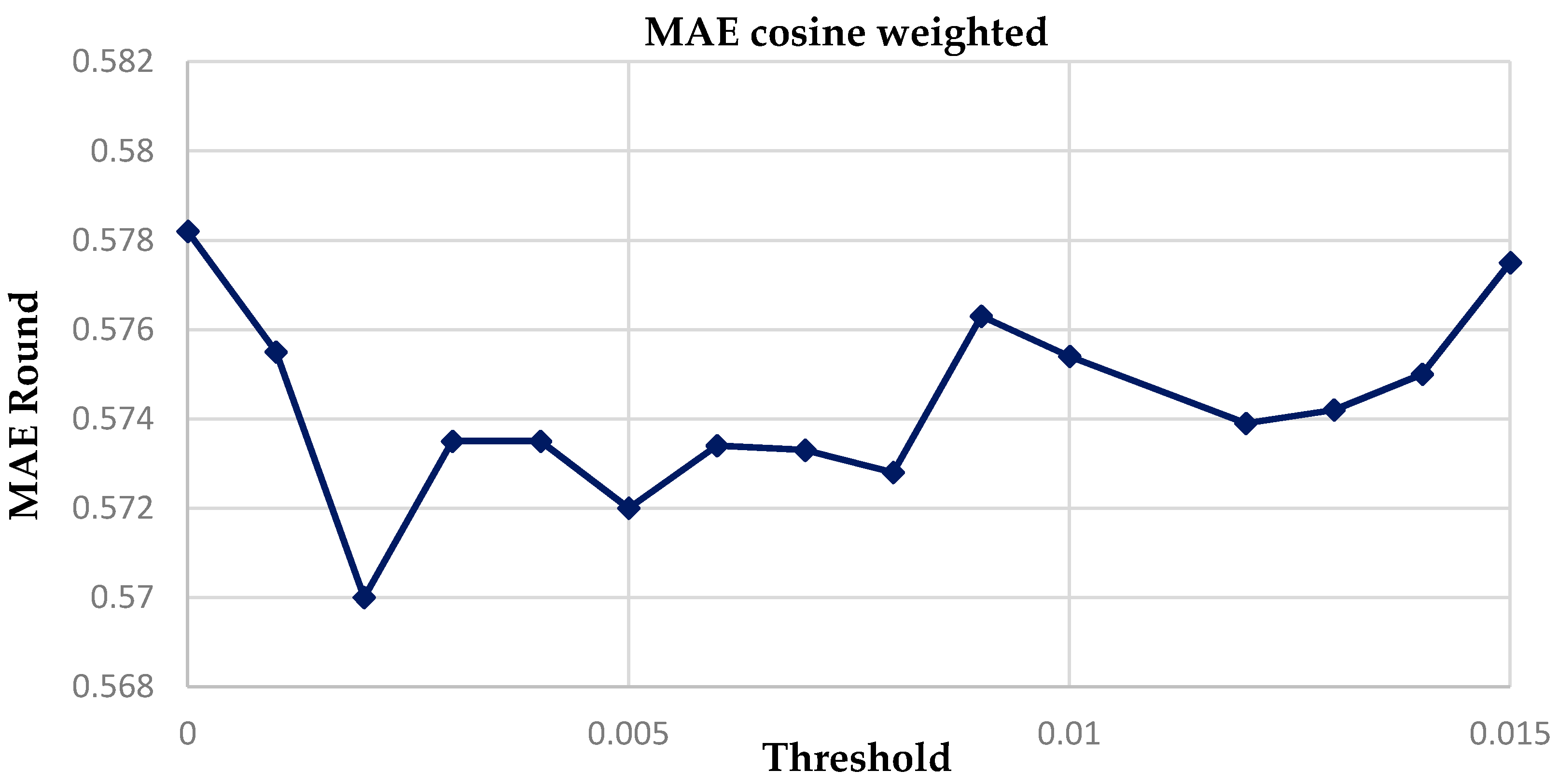
Cosine Weighted	0.5719	0.005	0.8169

shows that the lowest Mean Average error is 0.5719 for the cosine weighted similarity with a threshold of 0.005. It also has the most accuracy and least alpha and beta error values. Moreover, the variation of the graph of the MAE of KP weighted and cosine weighted vs. threshold shows that the MAE for the cosine weighted stays low for a wider range of threshold, from 0 to 0.015, while the value of the MAE shoots up almost immediately. Similar results are true in regard to the accuracy. This shows that the cosine function seems to provide greater stability for different student data for a fixed threshold value as compared to the KP function. This hypothesis will be tested later.

Near the region of the threshold = 0.005 from 0 to 0.01 in steps of size 0.001 we checked to find a threshold that gives more accurate results.

Figure 8 shows that the MAE Least squares estimation for threshold value = 0.002. The confusion matrix for an analysis of our prediction as to whether students get a grade more than 3 (“A” or “B”) is as follows.

4.2. Comparison with a Regression Analysis

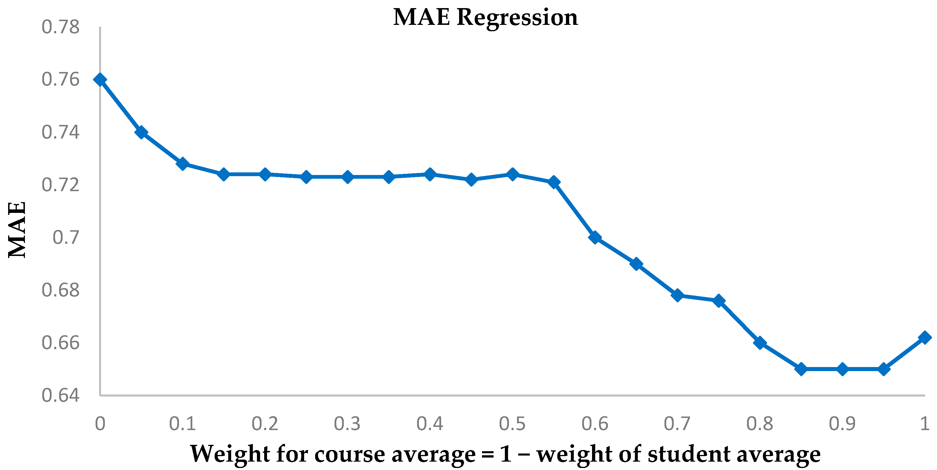
We assume a linear model for the prediction of a students’ grade in a future course, based on the student’s mean performance in his/her present courses and the average grade of the future course. The sum of the weights assigned equals one and is tested for different weights. The results for accuracy and MAE are plotted for a five-fold analysis. The weight for course average is increased in steps of 0.05. The tests carried out are for ensuring accuracy in predicting whether the student’s grade is below grade 3. The related results are shown in Figure 9 and Figure 10.

The Confusion Matrix for most accuracy using regression is shown in

Table 7. Confusion Matrix for regression analysis with highest accuracy.

MAE = 0.7029	AG < 3	AG ≥ 3	Acc
Folds = 5
w = 0.45
PG < 3	125	119	0.7594
PG ≥ 3	47	399	Total = 690

PG: Predicted Grade, AG: Actual Grade, ACC: Accuracy, AE: Alpha Error, BE: Beta Error.

.

The highest accuracy is at 76% with weight = 0.45 for course average compared to our model’s accuracy at 82.04%. In addition, the value for least MAE is 0.6502 for weight = 0.9, significantly greater than our model’s least MAE at 0.5699. Hence, our model is a much improved method over classic regression. In addition, the weights for the regression model for highest MAE and least accuracy do not correspond, which shows that a standardized weight may not be applicable.

4.3. Testing Whether a Student Will Pass

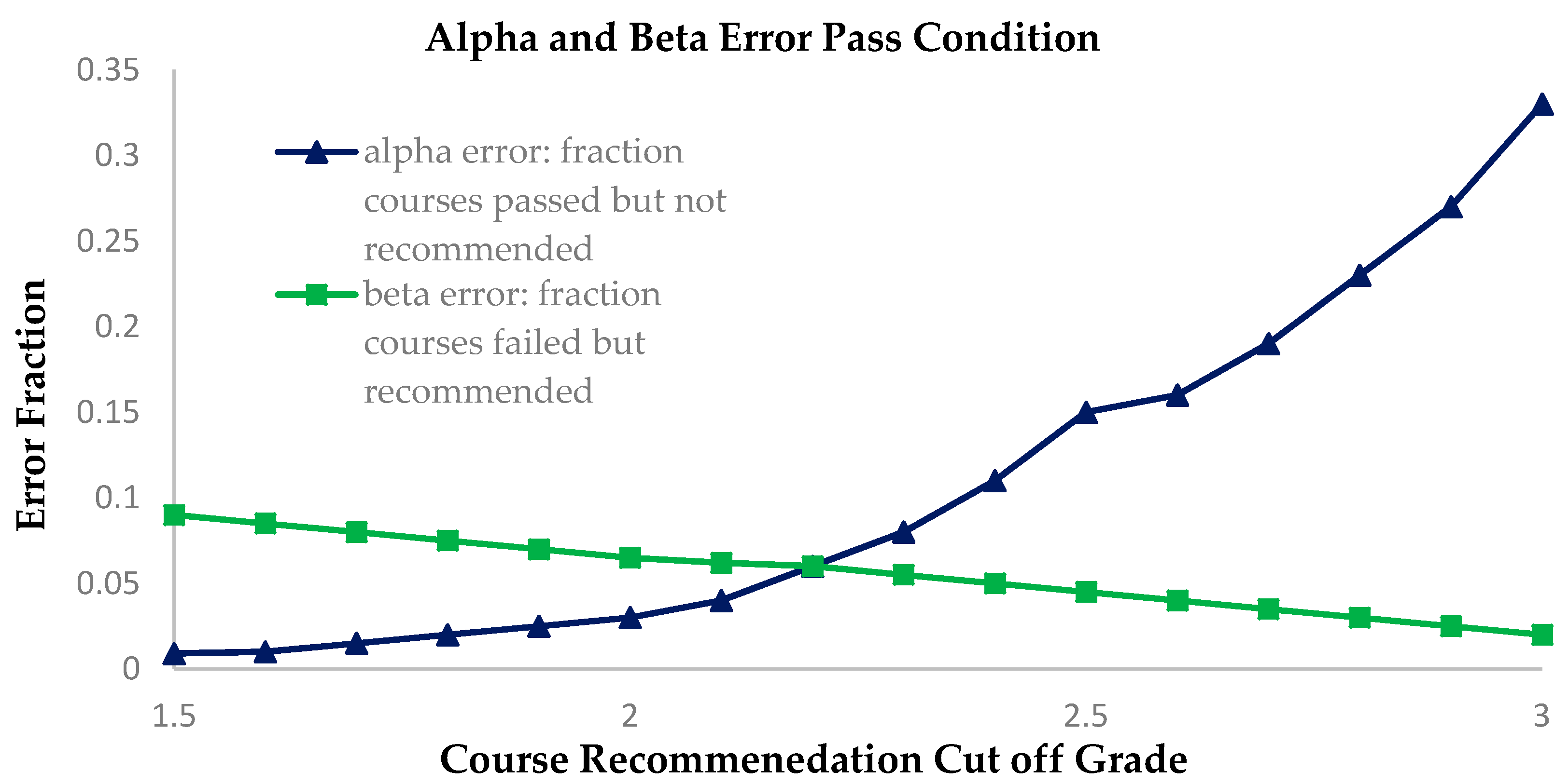
For this scenario, courses are recommended when the prediction is that the student will pass. The recommendation criteria are based on a minimum cutoff for the predicted grade. If the actual received grade of a student is 1, the student will fail. We chart the effect of our system for errors for different values of the cutoff grade and recommend courses only if the predicted grade is greater than the cutoff grade. The cutoff grade varies from 1.5 to 3 in steps of 0.1 shown as Figure 11.

We see that our method provides low values of error for a range of cutoff scores. Passing a course is a very important factor for a student. Hence it is essential to reduce the beta error for the students. This can be achieved by having a high cutoff grade for the recommendation system. However, this increases the alpha error of the system where we fail to recommend those courses in which the student passes.

Thus we reduce the diversity of the final course selection for the student. Therefore, there is a tradeoff between probability of passing the course and selecting from a wider pool of courses. We constructed the confusion matrix where we select the cutoff grade for recommendation. According to

Table 8. Confusion matrix for cutoff grade = 2 for courses with predicted grade ≥ 2.

MAE = 0.5501	AG < 2	AG = 2	Acc
Cutoff-Grade = 2
PG < 2	3	7	0.9055
PG ≥ 2	15	208	Total = 233

PG: Predicted Grade, AG: Actual Grade, ACC: Accuracy.

, the fraction of courses recommended = (208 + 15)/233 = 0.9570 out of 113 courses for years 3 and 4 equaling ~108 courses. To help students narrow their search pool we added a professor rating filter, such that it recommends only those courses where the Professor scores at least 2 points on a grade of 5. It acts as a quality assurance bar for course recommendation. If the professor has not been rated, or if the feedback information is not available, we consider just the predicted score as the basis for the recommendation without the rating filter. Now, we see that the total fraction of recommendations = (7 + 208)/233 = 0.9227. Hence, we recommend 113 × 0.4171 = 47 courses such that the average student has a 92.27% probability of passing any of these courses, and the professor’s rating is at least 2. Thus we ensure diversity in course selection as well as quality, while reducing the chance of failure for students. We see that the accuracy or errors of our selection are not significantly affected by the professor rating (in both cases the accuracy is above 90%).

4.4. Checking Effects of Professor Rating Filter on Accuracy of Predictions

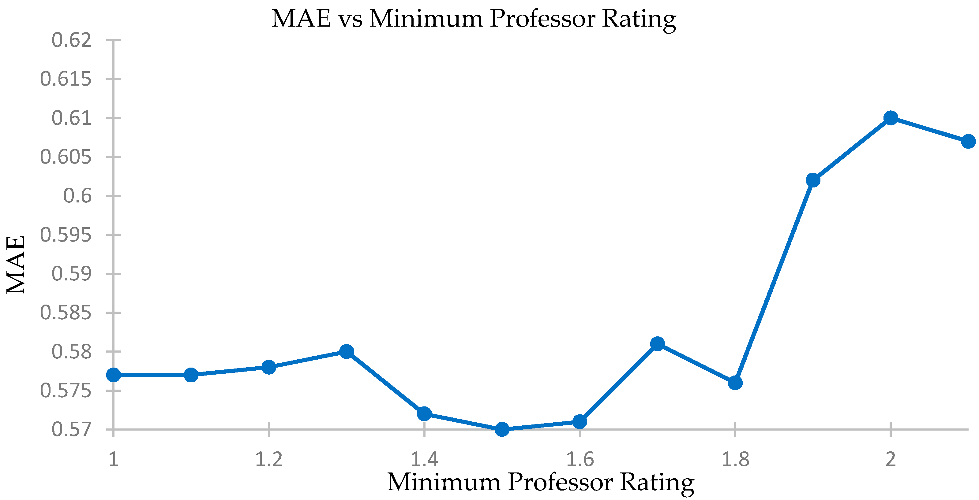
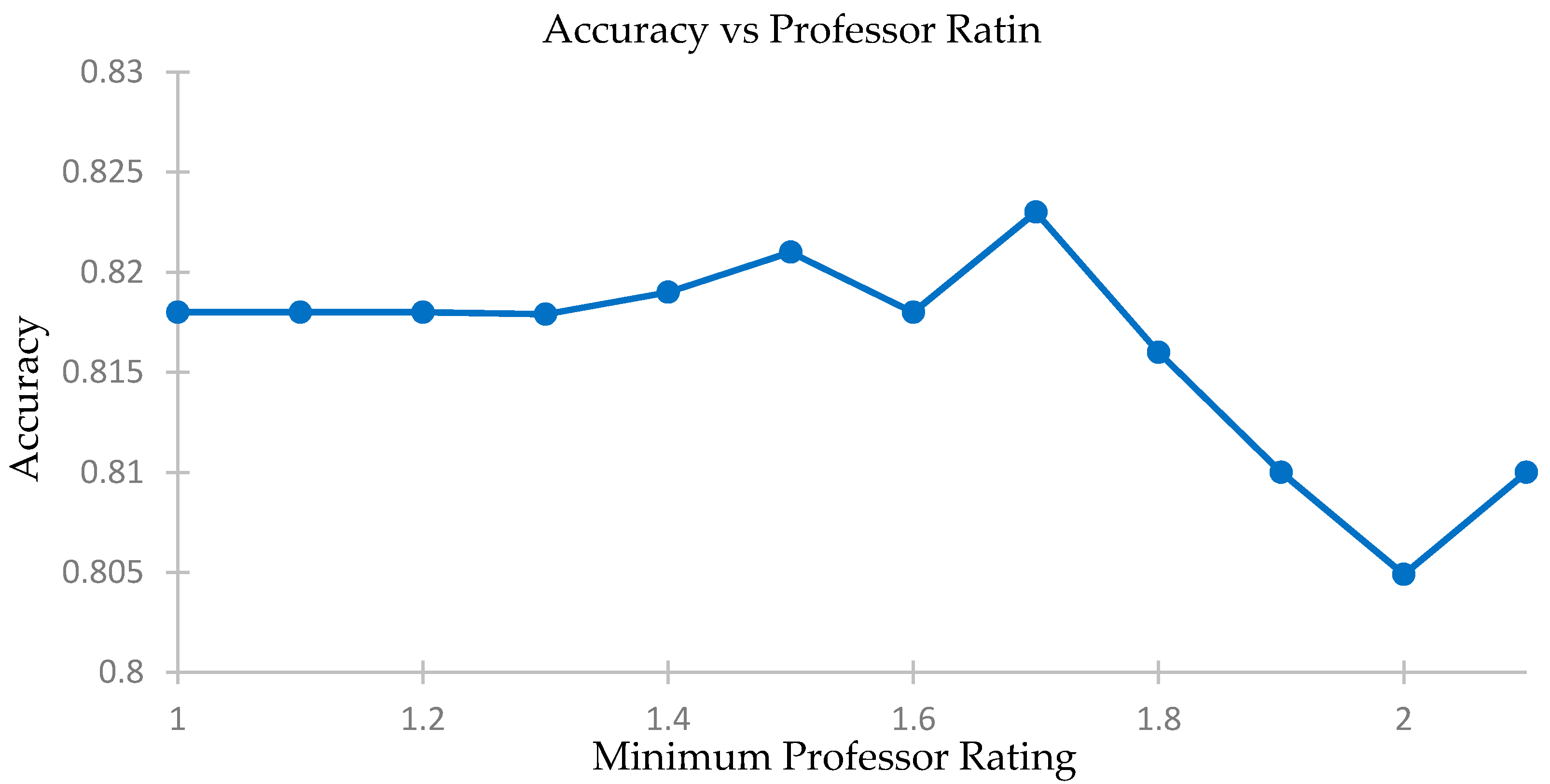
We compare the accuracy levels of our predictions for different minimum professor rating levels and select only those courses where the instructor secures a minimum score in the feedback report or is unrated and there is a weighted cosine analysis. We plot MAE and see the effects on the accuracy of our recommendation system using a five-fold accuracy vs. minimum professor rating threshold. The elated results are shown in

Table 9. Confusion matrix for course passed recommendation with professor rating filter.

MAE = 0.5733	AG < 2 (Fail Condition)	AG ≥ 2	Acc
Threshold = 0.002
Professor filter = 2
PG < 2 (fail condition)	1	3.2	0.9009
PG ≥ 2	6.8	90	Total = 101

PG: Predicted Grade, AG: Actual Grade, ACC: Accuracy.

, Figure 12 and Figure 13.

We see that the change in accuracy and MAE levels are not significant. The levels stay constant until a professor rating of about 1.8. The difference in best and worst accuracies is only 2%, while the difference in MAE is 0.04. Thus, the use of professor’s rating will not affect our prediction model, especially if the filter operates at below 1.8 for the professor rating.

5. Conclusions

This research uses the student and professor information of YZU University, Taiwan, to build and test a two-stage collaborative filtering model for course recommendations for students, with a filter for professor ratings. An initial collaborative filter based on the students’ departments is used. The second collaborative filter employs a clustering mechanism based on the Artificial Immune Network Theory to identify similar student groups, using the Karl Pearson and Cosine similarity coefficients for calculating affinities. This is followed by predicting the ratings of students using affinities between antibodies and antigens as weighting factors, and testing the results for various scenarios. We successfully demonstrate the effectiveness of employing the collaborative model and show that the use of a quality filter for professor ratings does not interfere with the predictions. The use of this model in a recommendation system could greatly help students identify courses where they may demonstrate greater aptitude and interest.

In the future, we may employ more feedback information from students for effective course selection. In addition, a model may be proposed for students for postgraduate students and freshmen. The use of a learning mechanism for tuning parameters for different departments may also find applications.