Variability in Mixed Conifer Spatial Structure Changes Understory Light Environments
by
 , ,
, ,
Jeffery B. Cannon
1,2,*,† ,
,
Wade T. Tinkham
2,
Ryan K. DeAngelis
1,
Edward M. Hill
2 and
Mike A. Battaglia
3 1
Colorado Forest Restoration Institute, Colorado State University, 1472 Campus Delivery, Fort Collins, CO 80526, USA
2
Department of Forest and Rangeland Stewardship, Colorado State University, 1472 Campus Delivery, Fort Collins, CO 80523, USA
3
USDA Forest Service, Rocky Mountain Research Station, 240 W. Prospect Road, Fort Collins, CO 80526, USA
*
Author to whom correspondence should be addressed.
†
Current affiliation: The Jones Center at Ichauway, 3988 Jones Center Drive, Newton, GA 39870, USA.
Forests 2019, 10(11), 1015; https://doi.org/10.3390/f10111015
Submission received: 3 September 2019
/
Revised: 8 November 2019
/
Accepted: 11 November 2019
/
Published: 13 November 2019
(This article belongs to the Special Issue Impacts of Complex Forest Structures on Tree Regeneration)
Abstract
:In fire-adapted conifer forests of the Western U.S., changing land use has led to increased forest densities and fuel conditions partly responsible for increasing the extent of high-severity wildfires in the region. In response, land managers often use mechanical thinning treatments to reduce fuels and increase overstory structural complexity, which can help improve stand resilience and restore complex spatial patterns that once characterized these stands. The outcomes of these treatments can vary greatly, resulting in a large gradient in aggregation of residual overstory trees. However, there is limited information on how a range of spatial outcomes from restoration treatments can influence structural complexity and tree regeneration dynamics in mixed conifer stands. In this study, we model understory light levels across a range of forest density in a stem-mapped dry mixed conifer forest and apply this model to simulated stem maps that are similar in residual basal area yet vary in degree of spatial complexity. We found that light availability was best modeled by residual stand density index and that consideration of forest structure at multiple spatial scales is important for predicting light availability. Second, we found that restoration treatments differing in spatial pattern may differ markedly in their achievement of objectives such as density reduction, maintenance of horizontal and tree size complexity, and creation of microsite conditions favorable to shade-intolerant species, with several notable tradeoffs. These conditions in turn have cascading effects on regeneration dynamics, treatment longevity, fire behavior, and resilience to disturbances. In our study, treatments with high aggregation of residual trees best balanced multiple objectives typically used in ponderosa pine and dry mixed conifer forests. Simulation studies that consider a wide range of possible spatial patterns can complement field studies and provide predictions of the impacts of mechanical treatments on a large range of potential ecological effects.
1. Introduction
In many fire-adapted conifer forests of the Western U.S., changes in land use activities and disturbance regimes such as logging, grazing, and fire suppression have led to increased forest densities and altered overstory composition [1]. In ponderosa pine-dominated (Pinus ponderosa Lawson and C. Lawson) forests of the Colorado Front Range, such changes have led to average overstory density increases of up to 350% in lower montane forests and nearly 140% in upper montane forests [2,3]. Increased horizontal and vertical continuity of canopy fuels, especially in lower montane forests, has led to uncharacteristic fire behavior [4,5]. Large and severe wildfires have far-reaching impacts on a host of ecological processes and services such as delayed forest recovery [4,6], increased understory invasibility [7], loss of organic matter and nutrients in soils [8], and degraded water quality [9,10]. To address these ecological threats, land managers often use fuel-reduction treatments employing mechanical thinning or prescribed fire. These treatments primarily emphasize changes in stand structure to increase forest resilience to future fire including reducing tree density; disrupting horizontal and vertical continuity of fuels to reduce fire hazard; and retaining old, large trees most likely to survive future fires [1,11,12,13].
Historically, many dry conifer forests of the Western U.S. were characterized by high variability in the fine-scale spatial structure of overstory trees—with stands composed of diverse elements such as large interspaces or openings, individual isolated trees, and groups of few to many trees due to the legacies of low- and mixed-severity fire regimes [14]. Fine-scale spatial heterogeneity of trees can contribute to an increase in forest resilience to future disturbances such as drought and fire [15], increase wildlife habitat value [16], and enhance understory diversity [17,18]. Therefore, in addition to fire mitigation objectives, many modern management practices often include objectives to restore fine-scale structural heterogeneity in these systems [1,16,19,20,21,22]. In contrast to traditional, even-spaced tree thinning that emphasizes timber production, restoration treatments often attempt to restore historical heterogeneous spatial patterns by using techniques such as variable tree spacing, opening creation, and tree group retention [23,24,25]. However, historical spatial patterns used as reference sites can vary considerably [14]. Futher, various implementation methods can lead to a range of outcomes in spatial pattern that may differ from treatment objectives which may vary considerably in their congruency with historical spatial patterns [13,14,20,26,27,28,29,30]. Decisions related to residual tree spatial pattern impact a number of important abiotic and biotic factors such as light availability, nutrient availability, and tree establishment and growth [31,32,33,34,35].
Although restoration treatments in ponderosa pine forests generally have goals to favor regeneration of ponderosa pine over other conifer species, retention of trees in more uniform patterns with dispersed shade may instead promote growing conditions favorable to more shade-tolerant species such as Douglas-fir (Pseudotsuga menziesii (Mirb.) Franco) [36,37,38]. In addition, various implementation methods to alter spatial heterogeneity (e.g., individual versus group selection) may impact other important factors such as overstory vertical complexity, microsite diversity, and fire characteristics [13,39,40], which are critical to regeneration dynamics and create uncertainty regarding the trajectory and longevity of many restoration treatments [41]. For example, Ma et al. [39] found higher variability in microsite conditions with greater overstory structural variability in mixed conifer forests of the Sierra Nevada. However, the study does not provide quantitative data linking how a range of tree spatial patterns alters environmental conditions relevant to developing predictions of stand trajectories. In this study, we model understory light levels across a range of forest density in a stem-mapped mixed conifer forest and apply this model to simulated stem maps similar in residual basal area yet varying in the degree of spatial complexity. We use the outputs of these simulations to assess how decisions related to residual overstory spatial patterns influence (1) overstory structural complexity and (2) understory light availability and variability.
2. Methods
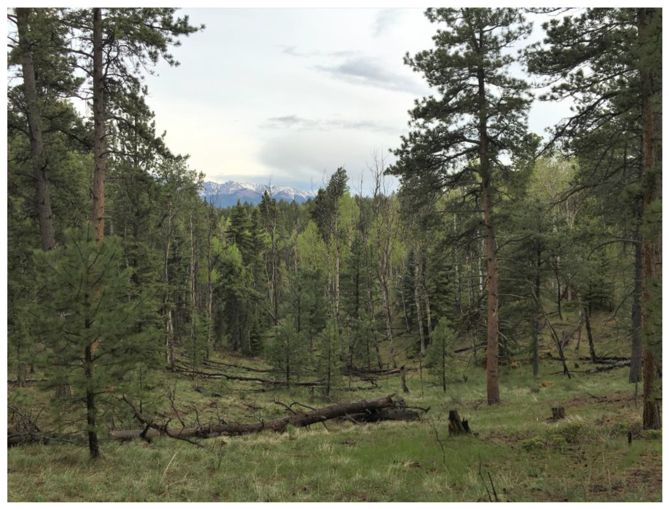
We conducted this study in a mixed conifer forest on the Pike-San Isabel National Forest in Colorado, USA (39.010°, −105.005°). Elevation at the study site ranges from 2795 to 2830 meters. The study area is composed of two forest communities that are determined by local topography. Drier, south-facing slopes are dominated by ponderosa pine with intermixed quaking aspen (Populus tremuloides Michx.) and limber pine (Pinus flexilis James). Wetter, north-facing slopes are dominated by Engelmann spruce (Picea engelmannii Parry ex Engelm.) and Douglas-fir (Figure 1). We mapped all trees within a 17.6 ha study area using measurement standards adopted from a broader global network of forest dynamics plots [42]. High-precision reference locations were established along the site perimeter using a Topcon HiPer-Ga real-time kinetic global positioning system (Topcon Corp., Livermore, California, USA; ±10 mm horizontal). From the reference locations, a Pentax PCS-515 laser total station (TI Asahi Co., Saitama, Japan; ±3 mm horizontal) was geolocated and referenced to true north and used to establish a square 20 × 20 m set of grid cells across the site. Grid cells were then used for locating all overstory trees and sampling locations. The perimeter of each cell created by the grid was framed with measuring tapes and used to record the location, species, diameter at breast height (dbh) for over 15,000 live trees exceeding 1 cm dbh. No tree was ever estimated more than 10 m from the framing tapes, resulting in an estimated RMSE of ±15 cm of the true horizontal location. Because treatment objectives in dry conifer forests of the region often include explicit goals for increasing spatial heterogeneity [16,19,43,44], we focus analyses on the 11.0 ha of drier south-facing slopes (Figure 2).
2.1. Modeling Light Availability
To estimate understory light availability across a density gradient, we selected 56 plots from a previously established set of approximately 400 plots from a related study (Tinkham, unpublished data). We selected plots within the dry mixed conifer portion of the stand (Figure 2) and stratified a gradient of basal area (ranging from 3 to 41 m2 ha−1 as measured from a 15 m fixed radius). In July 2017, we captured canopy photographs in the center of each plot using a 24 megapixel mirrorless DSLR camera with 180° hemispherical lens mounted on a self-leveling gyroscope and tripod (Compact OMount, Regent Instruments, Inc,. Quebec, Canada). We took photographs at dawn or dusk to produce a clear contrast between canopy and sky, with the camera mounted at 1.5 m in height and oriented toward true north. We classified each image as canopy and sky pixels using threshold grey values in Gap Light Analyzer [45]. We transferred classified photos to Winscanopy software (Regent Instruments, Quebec, Canada) and modeled understory solar radiation as photosynthetically active mean growing season photon flux density (PPFD; μmol m−2 s−1). To parameterize Winscanopy, we modeled understory radiation during the growing season (May–September) at an average elevation of 2810 m, and we assumed a solar constant of 1353 μmol m−2 s−1 [46], an atmospheric transmissivity of 0.622 (mean value for Colorado Springs, CO between May and September) [47], and a standard overcast sky diffuse light model [48]. To facilitate comparison with other studies, we converted all PPFD measurements to proportion of full sun (FS) by dividing radiation values by the maximum radiation modeled for the site of 577.4 μmol m−2 s−1.
Understory light availability depends on a number of forest structural attributes such as canopy cover, tree density, tree height and vertical stratification, canopy architecture, and tree spatial pattern [31,32,49]. To model how forest structure impacts understory light availability, we used a model selection approach to describe how understory light availability, as modeled through canopy photography, varied as a function of forest structural attributes at a range of spatial scales. We considered five basic overstory structural metrics including basal area (BA; m2 ha−1), tree density (all stems > 12.7 cm, D13; stems ha−1), large tree density (stems > 25.4 cm, D25; stems ha−1), stand density index (SDI; 25 cm stem equivalents ha−1) using the Shaw [50] method, and neighborhood index (NI). Neighborhood index and similar metrics have been used as proxies for tree competition (e.g., [51]), and the metric is based on tree size (BA), but trees are weighted as a function of distance from the observation point (plot center), implicitly including a spatial component in this metric. We calculated the neighborhood index for each plot center using the following equation:
where NIr is the neighborhood index of a plot with radius r, BAi is the basal area of the ith tree within radius r, di is the distance (in m) of the ith tree from the plot center for all n trees within radius r, and Ar is the area (in ha) of the plot. For all plots, we calculated each of the five overstory metrics at multiple scales, ranging from 3 to 30 m in radius (in 2 m increments). Next, we modeled light availability as a function of overstory structural metrics at a range of scales through a model selection procedure to determine what metric and scales best describe understory light availability. Structural metrics compared included BA, D13, D25, SDI, NI. We modeled light availability using each structural metric measured at a range of scales, and included both single- and dual-scale models. For single-scale linear models, light availability took the following form:
where ms is each structural metric (BA, D13, D25, SDI, NI) at scale s. Because light availability is typically non-linearly related to tree density [52,53] and because our calculation of light availability is a proportion bounded from 0 to 1, we modeled light availability using a beta regression with a natural log link using the betareg package in R with parameter optimization via the BFGS gradient method [54]. Spatial patterns such as edge effects may influence light availability, so we also generated dual-scale models that considered each structural metric as measured at two scales. Dual-scale linear models took the following form:
where ms is each structural metric as measured at scale s, ms′ is each structural metric at scale s′ for all scales where s < s′. Thus, these models included each forest metric at a small scale, s, and a larger scale s′. After combining five structural metrics (BA, D13, D25, SDI, NI), two model forms (single- and dual-scale), and scales between 2 to 30 m (every 2 m), we generated 75 single-scale models (5 structural metrics × 15 scales), and 525 dual-scale models (5 metrics × 105 combinations of s and s′). To select the combination of scales and metrics that best predicted understory light availability, we calculated and compared Akaike information criterion (AIC) for all 600 models [55].
2.2. Simulating Restoration Treatments
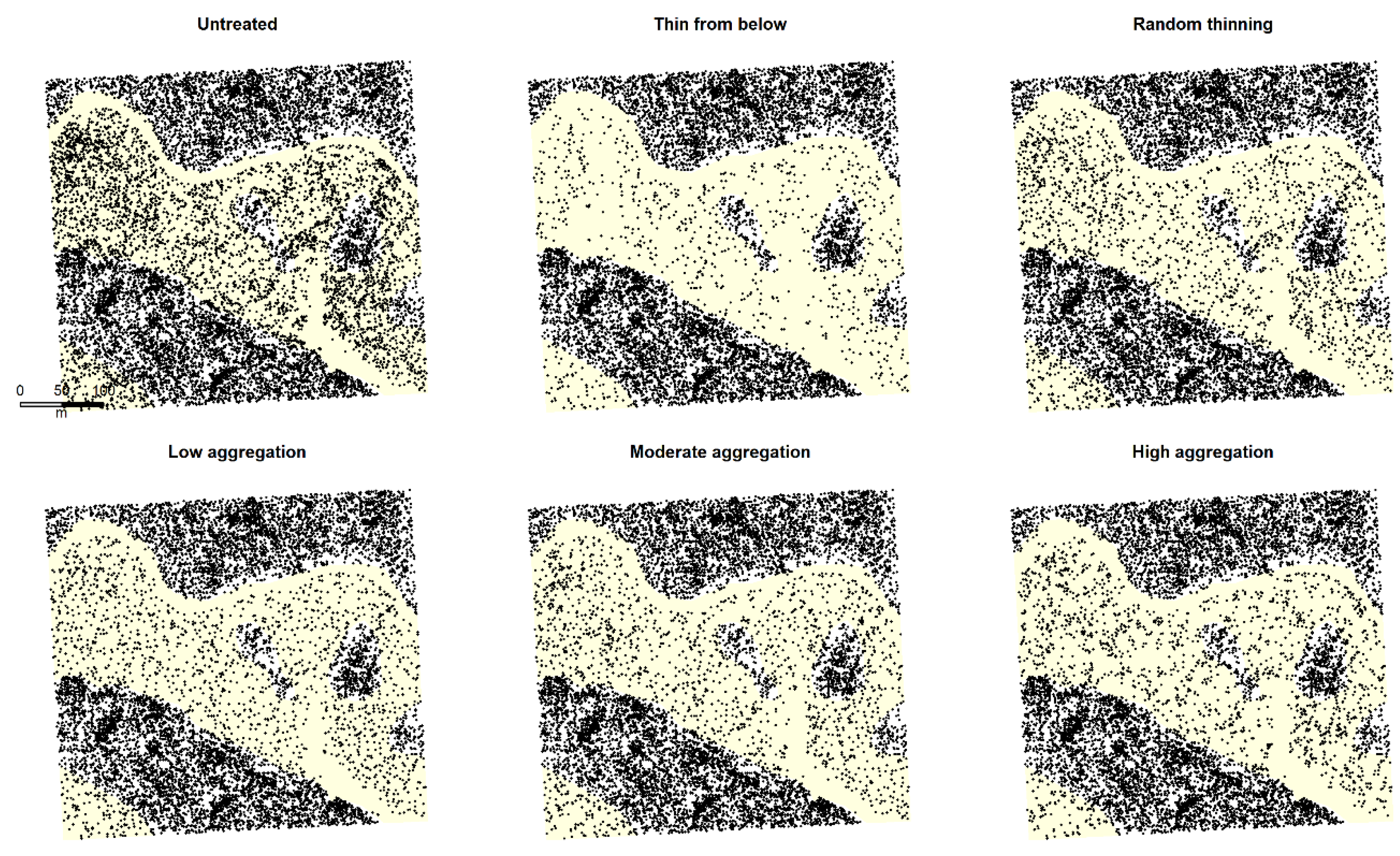
To assess how simulated treatments varying in spatial complexity changed the distribution of light availability, we generated stem maps simulating a range of treatment outcomes and applied the best model of light availability obtained in the above analysis. To simulate treatments varying in spatial pattern, we used the untreated stem map to simulate treatments that were similar in overall residual basal area, yet differing in tree spatial patterns including thinning from below, thinning overstory trees randomly, and restoration treatments varying in tree group size distributions (Figure 2, Table 1). Previous studies identify groups of trees as those with the potential for trees to develop interlocking crowns and continuous canopy, which in several studies of ponderosa pine is often represented as those with less than approximately 6 m spacing (e.g., [56,57]). In this study, we also used an intertree distance of 6 m based on the approximate 2.6–3.4 m crown radius range predicted from allometric equations linking tree diameter to crown radius [57] when trees reach the larger range of sizes noted at the site of 40–60 cm, and in the upper range of sizes noted in historical reconstructions of the region [2]. In addition, we use the term “group size” to refer to the number of individual trees in a group, rather than the areal coverage of tree groups which is more commonly referred to as “tree patch size” (e.g., [20]).
For each mechanical thinning simulation, we used a target basal area of 11.5 m2 ha−1 (Table 1). These values were chosen based on guidelines recommended for the region [19] and a silvicultural prescription developed for the site. We conducted 10 simulations for each stochastic thinning treatment. Example simulations for each treatment are shown in Figure 2. To simulate random thinning, we thinned all small trees (< 12.7 cm, < 5 in.) to a density of 40 ha−1 and then randomly selected larger trees for removal to reach the basal area target. To simulate thinning from below, we thinned starting with the smallest trees and proceeded to larger trees until the basal area target was reached.
To simulate more spatially complex restoration treatments, we first thinned small trees randomly to 40 ha−1, but overstory trees were thinned with varying degrees of spatial aggregation to a range of target tree group sizes (Table 1). We conducted 10 restoration simulations each with low, moderate, and high target levels of tree aggregation (Table 1), following Tinkham et al. [29]. We developed an algorithm in R that thins trees to the desired basal area, while reaching tree group size targets. The algorithm selects a tree in the stem map to initiate each group. The tree is randomly selected from a weighted probability of dbh in cm raised to the 1.6 power to simulate anchoring trees off of large existing trees (sensu [58,59]). Trees with boles within 6 m of the initial tree bole are added to the group, and proximal trees are added iteratively until a target group size is reached. The intertree distance used here represents a 3 m crown radius delineated to represent the potential for interlocking and adjacent crowns as trees mature.
When a tree group is formed, stems within 6 m of any group members are removed, and another group is initiated until the target stand basal area and target group size distributions are reached. See https://github.com/jbcannon/ICO_thinning_simulation (accessed on 12 November 2019) for example program and Figure S1 for example animation.
2.3. Assessment of Structural Complexity and Light Availability
To assess how simulated restoration treatments achieved desired conditions of decreasing density while maintaining horizontal and tree size complexity, we calculated basal area, stem density, quadratic mean diameter, and tree group size distributions. We used Shannon’s equitability (EH) to assess changes in horizontal complexity. This metric is often used to assess evenness in species assemblages but can be applied to other aspects of forest structure to assess complexity [60]. We determined tree density in 20 × 20 m grid cells and binned density into five classes (0–100, 100–200, 200–300, 300–400, and > 400 trees ha−1). We then calculated EH using proportions of the stand in each density class using the following equation:
where pi is the proportion of each stand in density class i, resulting in an estimate of horizontal complexity ranging from 0 to 1, with 1 representing equal representation among the five density classes [61,62]. To assess changes in tree size complexity, we calculated a stand density index ratio using the Reinke [63] and Shaw [50] methods, a proxy for tree size complexity [64,65] using the following equation:
where, SC is size complexity, Di is the diameter of the ith tree, TPHi is the number of trees represented by the ith tree, Dq is the stand-level quadratic mean diameter, and TPH is the stand-level stem density [65]. Note that we subtract from 1 the equation presented in Shaw [65] so that size complexity approaches 0 for even-aged stands, and increases for uneven-aged stands as size variability increases. We also present diameter distributions of treatment simulations to assess changes in tree size complexity.
To infer how simulated restoration treatments alter light availability, variability, and high light conditions, we applied the best predictive model of light availability from above to each stem map to generate raster data predicting light availability. A small edge buffer (6 m) was applied to the stem map to eliminate edge effects. Summary statistics were calculated to compare treatment effects on mean light availability (mean FS), light availability coefficient of variation (FS CV), and the 75th percentile light availability.
3. Results
3.1. Modeling Overstory Structural Effects on Light Availability
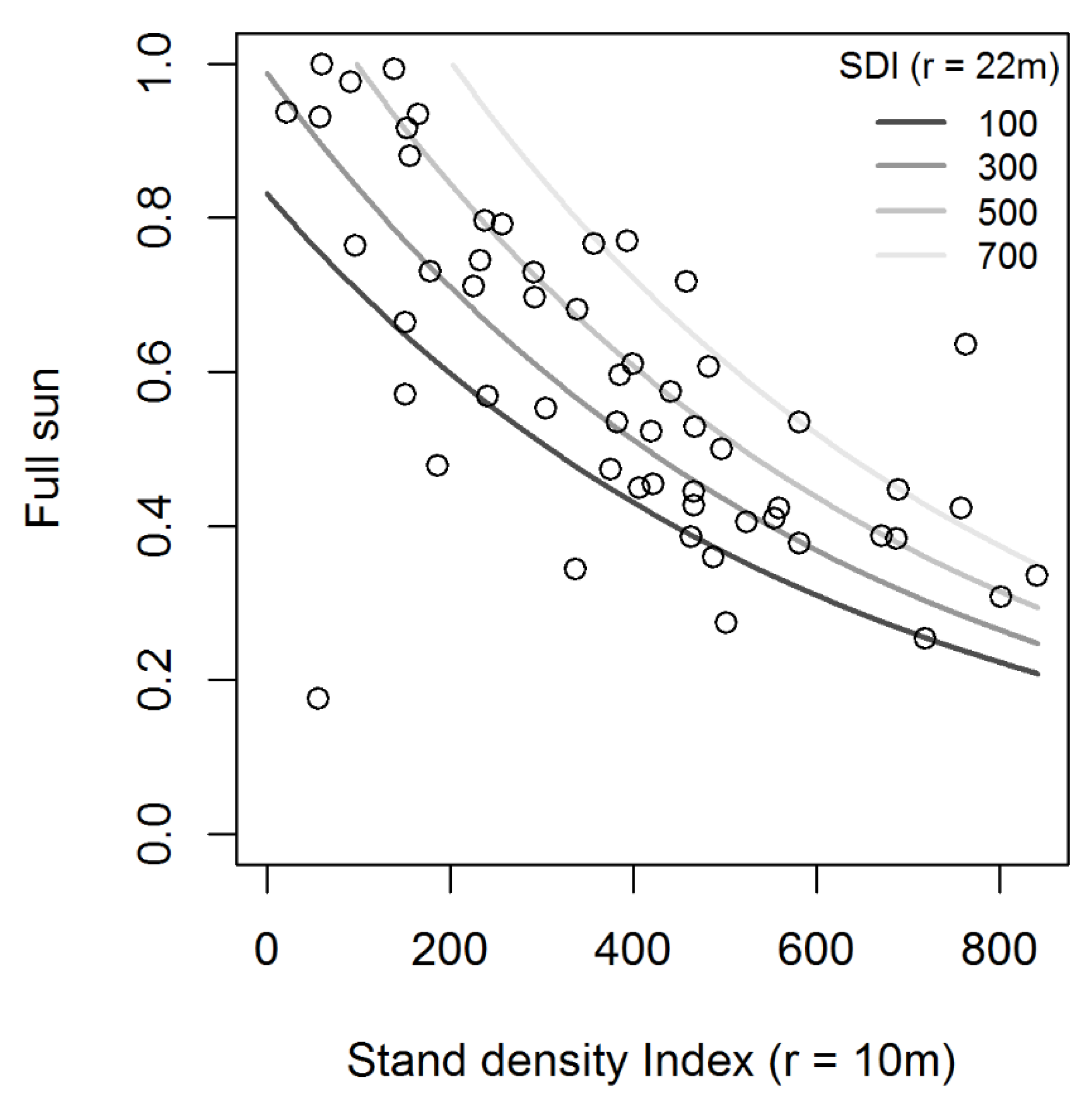
All of the top 10 best performing models included either stand density index or basal area as the metric capable of explaining the most variation in light availability and had pseudo−r2 values ranging from 0.4217 to 0.3512 (Table 2). The top three models (with ΔAIC < 2) consistently included a smaller scale of 10 m, and a larger scale between 22 and 24 m (Table 2). Although the models differ in the structural metric used (SDI versus BA), these metrics are closely correlated (r > 0.988) at all spatial scales. The best model of light availability included stand density index measured at 10 and 22 m (Table 3), which we used to predict light availability in subsequent simulation analysis. This model suggested that in dry mixed conifer stands, predicted light availability varies from 20% to 100% full sun, and that light availability increases rapidly when stand density index as measured at 10 m radius is reduced to < 300 to 500 ha−1 (Figure 3).
3.2. Effects of Treatment Simulations on Forest Structure and Complexity
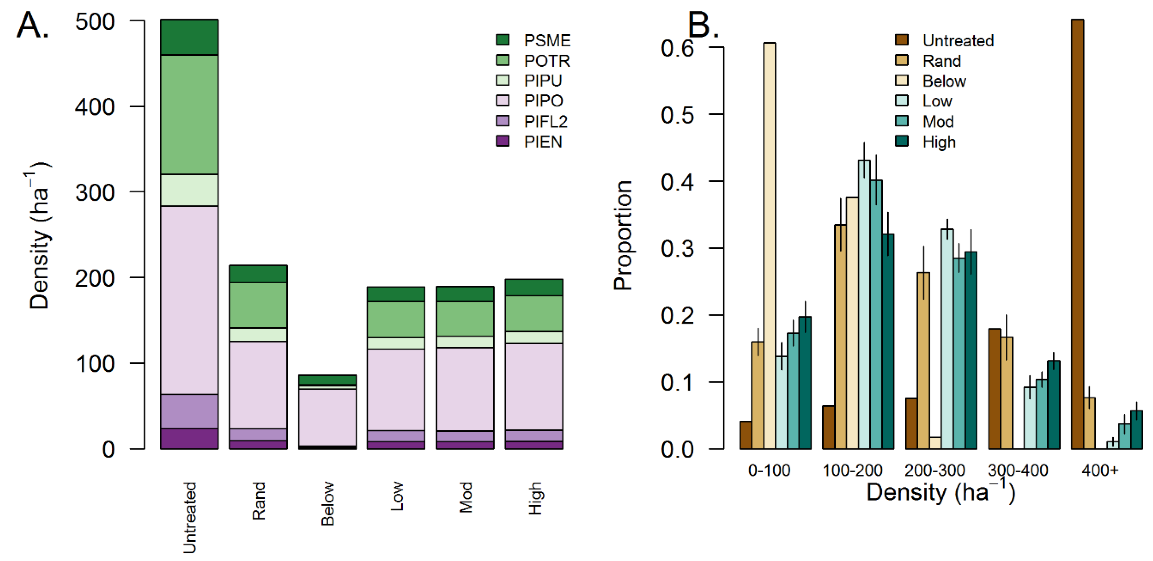
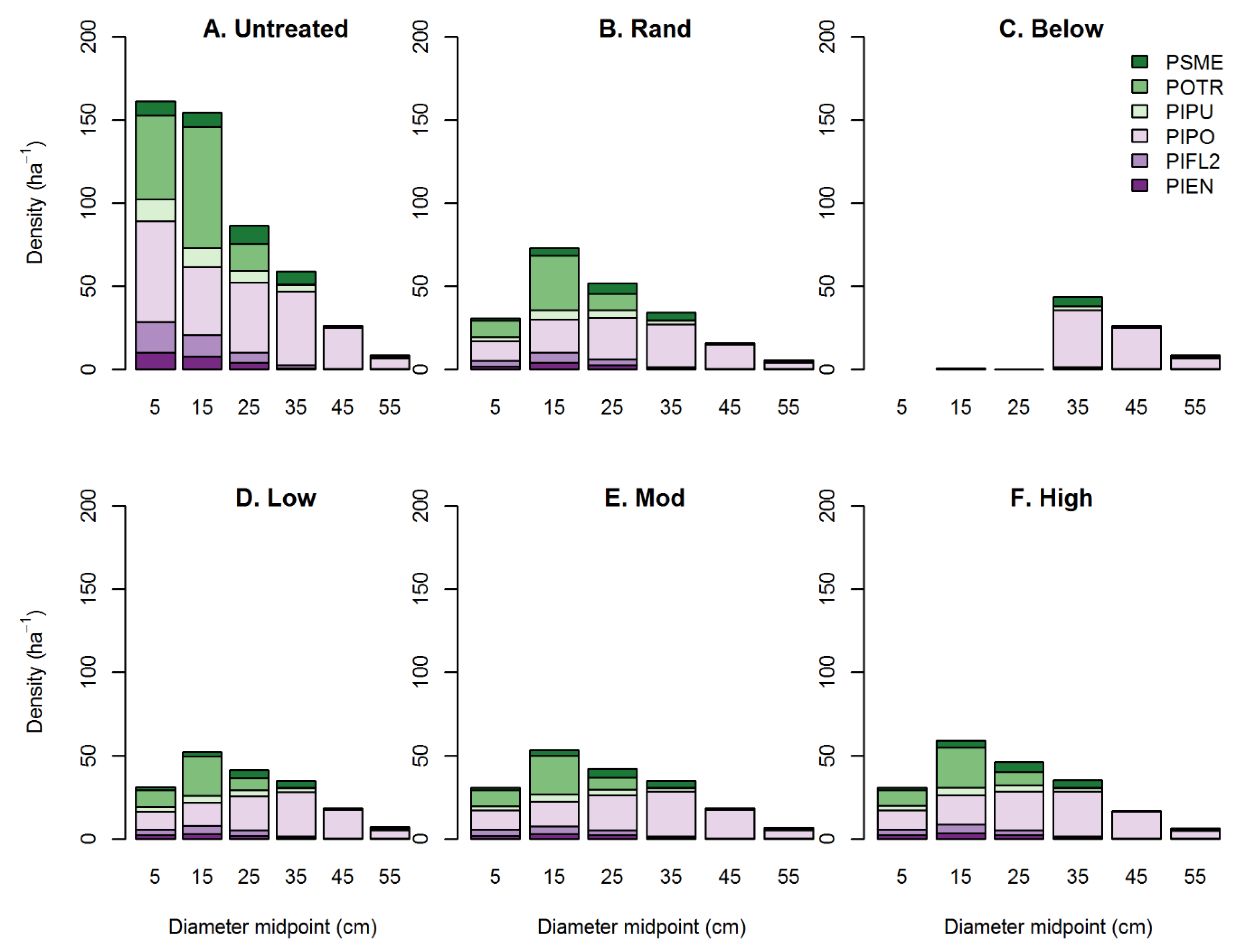
Treatment simulations resulted in stands with a constant basal area yet varying in other aspects of stand spatial structure such as density, tree group size distribution, horizontal complexity, and tree size complexity (Table 4). Simulations reduced basal area from an initial 20.0 m2 ha−1 to 11.5–11.6 m2 ha−1 in agreement with simulation constraints (Table 4). However, overall stem density varied among simulations. Simulated treatments reduced average tree density between 57% and 83%, with thinning from below resulting in the largest reduction (501 to 86 ha−1), random thinning resulting in the smallest reduction (501 to 214 ha−1), and aggregated treatments with moderate reductions (from 501 to approximately 195 ha−1, Table 4). We found that changes in tree group size distributions followed simulation parameters. Thinning from below the concentrated basal area in smaller tree group size classes, whereas random thinning led to greater evenness among tree group size classes (Table 4). Consistent with simulation constraints, we found that among the aggregated treatments, the low aggregation treatment exhibited the highest proportion of trees in smaller groups (1–4 trees per group), while the highly aggregated dry mixed conifer stands exhibited the greatest proportion of trees in larger groups (≥ 5 trees per group; Table 4). Simulations varied little in tree species composition and generally reduced species abundances proportionally to their initial abundance (Figure 4A). However, one exception was that thinning from below essentially eliminated species primarily represented by smaller diameter individuals such as quaking aspen (Figure 4A, Figure 5C).
Treatments varied in their ability to maintain or enhance aspects of horizontal and tree size complexity with thinning from below resulting in the largest reductions in complexity, while random and highly aggregated treatments best maintained both aspects of complexity (Table 4). Both untreated stands and thinning from below had the lowest horizontal complexity, with both stands having density equitability < 0.70 (Table 4) and > 60% of the total area with stem densities < 100 ha−1 or > 400 ha−1, respectively (Figure 4B). Random thinning had the highest horizontal complexity (0.93), and aggregated treatments had moderate horizontal complexity (from 0.78 to 0.91). Among the aggregated treatments, the highly aggregated treatment preserved the most area in the highest and lowest density classes (< 100 and > 400 ha−1), whereas the low- and moderately aggregated treatments resulted in a greater abundance of moderately dense classes (200–400 ha−1, Figure 4).
As expected, diameter distributions differed dramatically among untreated and treated stands with large reductions in density of stems < 30 cm in all simulated treatments (Figure 5) with the result that all treatments reduced tree size complexity (Table 4). However, the thin from below treatment especially reduced size complexity from an initial value of 0.11 in untreated stands to 0.01, whereas all other treatments only slightly reduced size complexity to between 0.07 and 0.08 (Table 4). Random thinning treatments retained more mid-sized stems (10–30 cm dbh) relative to all other treatments (Figure 5B). Thinning from below eliminated most stems < 30 cm (Figure 5C). Aggregated treatments were relatively similar in tree size complexity (ranging from 0.7 to 0.8). However, the high aggregation led to greater retention of mid-sized stems relative to the low- and moderately aggregated treatments and was thus most similar to the random thinning treatment (Figure 5D–F).
3.3. Effects of Treatment Simulations on Light Availability and Variability
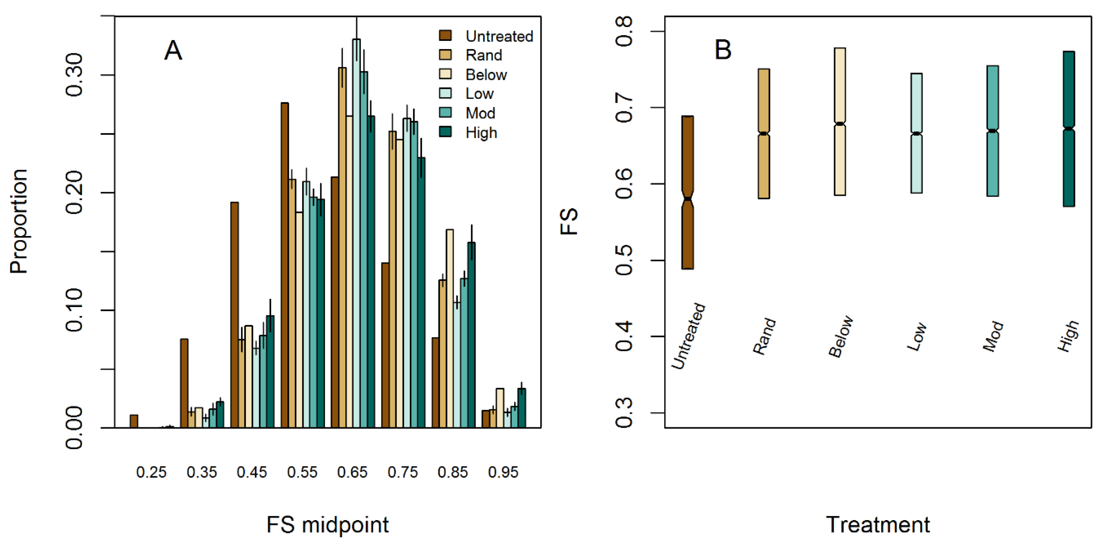
Increases in mean light availability were relatively similar across treatments, but treatments exhibited differences in within-stand variability in light levels (Table 5, Figure 6A). Mean light availability increased from 0.592 FS in the untreated stand to between 0.676 FS in the thin from below treatment to 0.665 in the low-aggregation treatment (Table 5). Variability of light levels paralleled results for within-stand horizontal complexity, where untreated stands had light levels primarily concentrated in the 0.40 to 0.60 FS range, whereas thinning from below concentrated a large area in the 0.70 to 1.0 FS range (Figure 6A). Among the aggregated treatments, the highly aggregated stand had the greatest variability in light availability (Table 5). Highly aggregated stands had more total area concentrated in the lowest (0.50) and highest (>0.80) light ranges compared to the other aggregated treatments. Conversely, the low- and moderate-aggregation treatments had a greater proportion of area concentrated in moderate light levels (0.50–0.80, Figure 6A). Changes in high-light availability increased in all treatments, with the 75th percentile FS increasing from 0.689 in untreated stands to between 0.745 to 0.778 (Table 5). Among the treated stands, 75th percentile FS was highest in the high-thin from below (0.778) and high-aggregation treatment (0.773), lowest in the low-aggregation treatment (0.745), and moderate in the random thinning and moderate-aggregation treatment (0.755) (Table 5).
4. Discussion
This study highlights how residual overstory spatial patterns have cascading impacts in mixed conifer forests such as altering the light environment and components of overstory structure such density, composition, and tree size complexity. The use of multi-scale models in predicting understory light transmittance from different forest structural metrics reveals an impactful spatial dependence. The 10 best performing models from our study highlight the importance of considering forest structure at two scales in heterogeneous forests. The larger scales (22–24 m) correspond approximately to the dominant overstory height in these stands, indicating that in spite of the high level of heterogeneity of forest structure in dry mixed conifer forests, light availability is in part driven by interactions between canopy height and latitude as has been found in temperate forests [49]. This spatial scale provides a logical approximation of the interaction between vegetation height and solar angle for representing the attenuation of light, which is approximated by basal area or stand density. Some studies have shown that a single radius (approximating vegetation height) can be used to model light availability when stands are homogeneous [66]. Conversely, in our study, a smaller scale (10 m radius) was also important to represent the highly variable fine-scale local forest density found within our study site. The natural clustering pattern found in most ponderosa pine sites [13,21] indicates that light availability in these forests is determined by both site-level density of trees, as well as fine scale differences in tree locations. Future modeling efforts could investigate the use of both distance-weighted metrics like the neighborhood index along with directional effects, as a tree along the solar incidence path should have a significantly stronger effect on light attenuation.
Our study demonstrated that while similar levels of density reduction can result in similar mean light availability, the range and variability of this resource differs due to the differences in overstory spatial pattern (Figure 6B). Increasing the degree of spatial aggregation within a treatment tended to increase variability in understory light availability. This is supported by both Martens et al. [67] and Battaglia et al. [31] who found that light variability increases when residual canopy structure is aggregated for both piñon pine (Pinus edulis Engelm.) and longleaf pine (Pinus palustris Mill.) forests, respectively. Our low-aggregation simulations extend this finding and indicate that when mechanical treatments decrease structural complexity, light variability can also be decreased relative to untreated stands. Such results highlight that a large range of ecological outcomes may occur across gradients of spatial pattern.
We found a non-linear regression best explained the relationship between basal area and light availability in dry mixed conifer stands (Figure 3 and Figure 6B), which has important implications for achieving ecological and management objectives related to structural variability and treatment longevity. A study by Vyse et al. [38] demonstrated greater survival of ponderosa pine seedlings over more shade-tolerant species when light availability exceeded approximately 65% full sun (crossover point irradiance (sensu [36])), and found that this crossover point occurred at 5.0 m2 ha−1 of basal area compared to an inflection point corresponding to between 10 and 20 m2 ha−1 in our study. Optimal light environments for ponderosa pine regeneration following traditional silvicultural regeneration treatments have been reported as 9–27.5 m diameter group-selection openings [68] or shelterwood treatments with 6–14 m2 ha−1 residual basal area (or not less than 4 m2 ha−1 [69]) in comparison with more continuous cover from alternative treatments [70]. Moreover, aggregated overstory retention is generally recommended to improve seedling growth of ponderosa pine [70], where openings provide adequate resource availability for ponderosa which can otherwise be significantly negatively affected by competition from saplings and larger canopy trees [33]. Yet in some cases, fuel hazard reduction treatments fall short of achieving the requisite high levels of overstory aggregation [20,28,30], and instead, result in more uniform overstory retention which may favor shade-tolerant species such as Douglas-fir [38]. Uniform overstory retention may thereby reduce the longevity of treatments with an objective to reduce ladder fuels [41]. Although exact light intensities and gap structures necessary to favor shade-intolerant species will differ by region, forest type, and species under consideration, the general finding that large basal area reductions are necessary to favor ponderosa pine indicate that careful consideration of the placement, size, and frequency of overstory gaps (i.e., fine-scale spatial pattern) is critical to increasing the proportion of stands that favor ponderosa pine over more shade-tolerant species.
Increasing heterogeneity in overstory and light conditions gives rise to cascading effects on many abiotic and biotic parameters creating variable microsite conditions that may impact plant diversity, ponderosa pine regeneration, and stand resilience. In our study, the high aggregation treatments generated the largest area of high light conditions, with the highest 75th percentile light availability among all treatments. The relatively high-light environments within low-density stands or openings have been linked to high understory productivity, as well as high herbaceous diversity in stands dominated by ponderosa pine [18,71]. Furthermore, high microclimatic variability characterizes many mixed conifer forests [72] and has been implicated in fostering high understory herbaceous diversity [73]. Ponderosa pine regeneration will be driven, in part, by microenvironments with biophysical conditions that support favorable moisture availability over both space and time [74,75,76,77,78,79]. Light environments that have been shown to favor ponderosa density and survival include open areas of few to no trees, and areas with moderate to low canopy cover, especially from intermediate canopy trees (e.g., 6–30 cm dbh) [33], where temperature extremes are alleviated, moisture is retained, and vegetation competition is moderated relative to resource requirements of ponderosa. In our study, the highly aggregated treatment simulation led to high overstory structural complexity and variable light environment that may better support ponderosa pine regeneration. Previous studies report that light environments defined by canopy cover and structure may drive fine-scale biotic conditions relevant to regeneration such as litterfall distribution and depths, vegetation type and structure, rainfall interception and throughfall, temperature and wind patterns, seedfall patterns, seed- and tree-predatory wildlife habitat, and moisture and nutrient uptake [39]. Variability in light conditions is, therefore, indicative of variable resource quantity and distribution [32,80] for tree regeneration. Variation in light and corresponding resource environments can increase stand forest resilience by providing a diverse range of microenvironments (spatially and temporally) to support complex regeneration dynamics [81]. In addition, variable microsite habitats may support or limit different life-stages of trees, and lead to facilitative interactions for young trees and competitive interactions for older individuals [75,82,83].
Beyond ponderosa pine, many pine-dominated systems, especially those shaped by fire, are characterized by high levels of heterogeneity that can impact resource availability and stand regeneration processes. Old-growth longleaf pine systems exhibit patchy regeneration driven by intra-specific competition, fire, and hurricane mortality [84]. Gap size and position drive light availability and regeneration success in longleaf stands [85,86], and aggregated harvest patterns have been shown to increase resource availability at both local and stand scales [35]. Although our study found relatively similar mean-light levels at the stand scale across treatments examined, we found large variability in light availability following aggregated retention (e.g., more area with high light, and more area with low light). Similarly, in mature red pine (Pinus resinosa Aiton) stands, both light availability and variability increased with aggregated harvests [87]. Further, within-gap variation in light availability in moisture led to differences in photosynthetic rates among three northern Pinus species, indicating the potential for gap portioning in these systems [88]. In moisture limited Scots pine (Pinus sylvestris L.) systems, successful regeneration is often associated with small gaps that provide moderate shade and improve summer moisture conditions [89], highlighting that fine-scale microclimate variability can impact stand-dynamics.
Direct field measurements of changing light conditions are useful for understanding changes in light availability and variability under relatively simple mechanical prescriptions such as individual or group selection studies [31]. However, given the range of target conditions and outcomes of restoration in ponderosa pine and mixed conifer forests, simulation studies such as the one presented here provide a framework for understanding the impacts of a large range of restoration outcomes on an important abiotic gradient. Nevertheless, there are several limitations to use of treatment simulations. To focus analysis and interpretation on spatial patterns of overstory retention, our simulation model was based strictly on retention of specific overstory patterns and size structure and did not explicitly consider overstory composition, although results may differ if stands contain a large component of spatially aggregated species such as quaking aspen. Furthermore, our simple spatial simulation model was based on specific targets for retaining a distribution of tree group sizes. Although this model successfully simulated fine-scale spatial structure (Table 4), it did not include larger-scale considerations such as creation of large openings or retention of groups of trees greater than 20 individuals. Future work can improve upon existing efforts by realistically simulating typical tree marking practices such as anchoring from large trees, identifying and expanding existing gaps, and explicit incorporation of larger openings, or by comparing changes in light variability following actual treatments where spatial patterns were specified in the prescription. Fine-scale simulations can be integrated with coarser-scale simulation models under development [90] to address nuances of treatment implementation and outcomes at multiple scales. Furthermore, our study was opportunistically conducted in a stand where extensive stem mapping had taken place, and used an empirical model of light availability based on stand structure, which may vary in other ecosystems and locations that vary greatly in latitude, stand composition, and tree height [49].
5. Conclusions
In ponderosa pine and dry mixed conifer forests, management goals for restoration typically emphasize structural changes to increase resistance and resilience to disturbances. Some of these objectives include (1) reducing overstory density, (2) increasing horizontal complexity, (3) maintaining tree size complexity, and (4) reducing the potential for regeneration by shade-tolerant species, such as Douglas-fir, that can act as ladder fuels and reduce treatment longevity [91]. Our results suggest that even with similar reductions in basal area, treatment prescriptions that differ in spatial pattern may differ markedly in their congruence with each of these goals, exhibiting important trade-offs among objectives related to tree density, structural complexity, and light environment. Thinning from below resulted in the largest reduction in overstory density, yet led to the largest reductions in structural complexity due to removal of all small stems. Conversely, random thinning maintained much of the existing horizontal and tree size complexity, yet resulted in modest density reductions and provided less with high light availability. Because the aggregation simulation was designed to anchor the formation of tree groups around large trees, the low-aggregation treatment was similar to an even-spaced thinning treatment and was dominated by single trees and small groups of trees, and was thus relatively uniform, resulting in relatively low horizontal complexity, light variability, and the least area with high-light availability. Conversely, the high-aggregation treatment after anchoring on larger trees retained many of the smaller surrounding trees creating spatial complexity while also maintaining tree size complexity. Thus, the high aggregation treatment balanced several objectives resulting in moderate density, relatively high horizontal and size complexity, and among the highest light variability and area with high-light availability. Treatments intentionally designed to create a wide distribution of tree group sizes may best meet restoration objectives and improve resilience in ponderosa pine forests.
Supplementary Materials
The following are available online at https://www.mdpi.com/1999-4907/10/11/1015/s1, Figure S1: Animation demonstrating tree group selection algorithm in 4 ha area.
Author Contributions
Conceptualization: J.B.C., M.A.B., and R.K.D.; Methodology: J.B.C., R.K.D., W.T.T., and M.A.B.; Software: J.B.C. R.K.D., and W.T.T.; Validation: R.K.D., J.B.C., and W.T.T.; Formal analysis: J.B.C., R.K.D., and W.T.T.; Investigation: R.K.D., J.B.C., W.T.T.; Resources: J.B.C. and M.A.B.; Data curation: R.K.D., J.B.C., and W.T.T.; Writing–Original draft preparation: J.B.C., R.K.D., W.T.T., and E.M.H.; Writing—Review and editing: J.B.C., W.T.T., R.K.D., E.M.H., and M.A.B.; Visualization: J.B.C., R.K.D., and W.T.T.; Supervision: J.B.C.; Project administration: J.B.C.; Funding acquisition: J.B.C. and W.T.T.
Funding
This work was supported by a USDA McIntire-Stennis Capacity Grant (COL00509) and based upon work supported by the Natural Resources Conservation Service, U.S. Department of Agriculture, Conservation Effects Assessment Project (Grazing Lands Component) under number 68-3A75-17-470.
Acknowledgments
The authors would like to thank L. Scott Baggett and two anonymous reviewers for statistical review and helpful comments that improved the analysis and discussion. We also thank Jonas Feinstein for insightful conversations on this topic and Brian Osterholzer for assistance with fieldwork.
Conflicts of Interest
The authors declare no conflict of interest.
References
- Allen, C.D.; Savage, M.; Falk, D.A.; Suckling, K.F.; Thomas, W.; Schulke, T.; Stacey, P.B.; Morgan, P.; Hoffman, M.; Klingel, J.T. Ecological restoration of southwestern Ponderosa pine ecosystems: A broad perspective. Ecol. Appl. 2002, 12, 1418–1433. [Google Scholar] [CrossRef]
- Battaglia, M.A.; Gannon, B.; Brown, P.M.; Fornwalt, P.J.; Cheng, A.S.; Huckaby, L.S. Changes in forest structure since 1860 in ponderosa pine dominated forests in the Colorado and Wyoming Front Range, USA. For. Ecol. Manag. 2018, 422, 147–160. [Google Scholar] [CrossRef]
- Brown, P.M.; Battaglia, M.A.; Fornwalt, P.J.; Gannon, B.; Huckaby, L.S.; Julian, C.; Cheng, A.S. Historical (1860) forest structure in ponderosa pine forests of the northern Front Range, Colorado. Can. J. For. Res. 2015, 45, 1462–1473. [Google Scholar] [CrossRef]
- Fornwalt, P.J.; Huckaby, L.S.; Alton, S.K.; Kaufmann, M.R.; Brown, P.M.; Cheng, A.S. Did the 2002 hayman fire, Colorado, USA, burn with uncharacteristic severity? Fire Ecol. 2016, 12, 117–132. [Google Scholar] [CrossRef]
- Sherriff, R.L.; Platt, R.V.; Veblen, T.T.; Schoennagel, T.L.; Gartner, M.H. Historical, observed, and modeled wildfire severity in montane forests of the colorado front range. PLoS ONE 2014, 9, e106971. [Google Scholar] [CrossRef]
- Chambers, M.E.; Fornwalt, P.J.; Malone, S.L.; Battaglia, M.A. Patterns of conifer regeneration following high severity wildfire in ponderosa pine—dominated forests of the Colorado Front Range. For. Ecol. Manag. 2016, 378, 57–67. [Google Scholar] [CrossRef]
- Griffis, K.L.; Crawford, J.A.; Wagner, M.R.; Moir, W.H. Understory response to management treatments in northern Arizona ponderosa pine forests. For. Ecol. Manag. 2001, 146, 239–245. [Google Scholar] [CrossRef]
- Certini, G. Effects of fire on properties of forest soils: A review. Oecologica 2005, 143, 1–10. [Google Scholar] [CrossRef]
- Moody, J.A.; Martin, D.A. Hydrologic and Sedimentologic Response of Two Burned Watersheds in CO; US Geological Survey Water Resources Investigation Report 01-4122; US Geological Survey: Denver, CO, USA.
- Rhoades, C.C.; Entwistle, D.; Butler, D. The influence of wildfire extent and severity on streamwater chemistry, sediment and temperature following the Hayman Fire, Colorado. Int. J. Wildl. Fire 2011, 20, 430–442. [Google Scholar] [CrossRef]
- Agee, J.K.; Skinner, C.N. Basic principles of forest fuel reduction treatments. For. Ecol. Manag. 2005, 211, 83–96. [Google Scholar] [CrossRef]
- Fulé, P.Z.; Crouse, J.E.; Roccaforte, J.P.; Kalies, E.L. Do thinning and/or burning treatments in western USA ponderosa or Jeffrey pine-dominated forests help restore natural fire behavior? For. Ecol. Manag. 2012, 269, 68–81. [Google Scholar] [CrossRef]
- Ziegler, J.P.; Hoffman, C.; Battaglia, M.; Mell, W. Spatially explicit measurements of forest structure and fire behavior following restoration treatments in dry forests. For. Ecol. Manag. 2017, 386, 1–12. [Google Scholar] [CrossRef]
- Larson, A.J.; Churchill, D. Tree spatial patterns in fire-frequent forests of western North America, including mechanisms of pattern formation and implications for designing fuel reduction and restoration treatments. For. Ecol. Manag. 2012, 267, 74–92. [Google Scholar] [CrossRef]
- Hessburg, P.F.; Agee, J.K.; Franklin, J.F. Dry forests and wildland fires of the inland Northwest USA: Contrasting the landscape ecology of the pre-settlement and modern eras. For. Ecol. Manag. 2005, 211, 117–139. [Google Scholar] [CrossRef]
- Reynolds, R.T.; Sánchez Meador, A.J.; Youtz, J.A.; Nicolet, T.; Matonis, M.S.; Jackson, P.L.; Delorenzo, D.G.; Graves, A.D.; Richard, T.; Meador, S.; et al. Restoring Composition and Structure in Southwestern Frequent-Fire Forests: A science-based framework for improving ecosystem resiliency. Gen. Tech. Rep. PSW-GTR-220 2013, 86, 310. [Google Scholar]
- Dodson, E.K.; Peterson, D.W. Dry coniferous forest restoration and understory plant diversity: The importance of community heterogeneity and the scale of observation. For. Ecol. Manag. 2010, 260, 1702–1707. [Google Scholar] [CrossRef]
- Matonis, M.S.; Binkley, D. Not just about the trees: Key role of mosaic-meadows in restoration of ponderosa pine ecosystems. For. Ecol. Manag. 2018, 411, 120–131. [Google Scholar] [CrossRef]
- Addington, R.N.; Aplet, G.H.; Battaglia, M.A.; Briggs, J.S.; Brown, P.M.; Cheng, A.S.; Dickinson, Y.; Feinstein, J.A.; Fornwalt, P.J.; Gannon, B.; et al. Principles and Practices for the Restoration of Ponderosa Pine and Dry Mixed Conifer Forests of the Colorado Front Range. Gen. Tech. Rep. RMRS-GTR-373; U.S. Department of Agriculture, Forest Service, Rocky Mountain Research Station: Fort Collins, CO, USA, 2018.
- Cannon, J.B.; Barrett, K.J.; Gannon, B.M.; Addington, R.N.; Battaglia, M.A.; Fornwalt, P.J.; Aplet, G.H.; Cheng, A.S.; Underhill, J.L.; Briggs, J.S.; et al. Collaborative restoration treatments on forest structure in ponderosa pine forests of Colorado. For. Ecol. Manag. 2018, 424, 191–204. [Google Scholar] [CrossRef]
- Churchill, D.J.; Carnwath, G.C.; Larson, A.J.; Jeronimo, S.A. Historical Forest Structure , Composition, and Spatial Pattern in Dry Conifer Forests of the Western Blue Mountains , Oregon; General Technical Report (GTR) PNW-GTR-956; Pacific Northwest Research Station: Portland, OR, USA, 2017; p. 93. [Google Scholar]
- Dickinson, Y. Landscape restoration of a forest with a historically mixed-severity fire regime: What was the historical landscape pattern of forest and openings? For. Ecol. Manag. 2014, 331, 264–271. [Google Scholar] [CrossRef]
- Larson, A.J.; Stover, K.C.; Keyes, C.R. Effects of restoration thinning on spatial heterogeneity in mixed-conifer forest. Can. J. For. Res. 2012, 42, 1505–1517. [Google Scholar] [CrossRef]
- Tuten, M.C.; Sánchez, A.; Fulé, P.Z. Forest Ecology and Management Ecological restoration and fine-scale forest structure regulation in southwestern ponderosa pine forests. For. Ecol. Manag. 2015, 348, 57–67. [Google Scholar] [CrossRef]
- Underhill, J.L.; Dickinson, Y.; Rudney, A.; Thinnes, J. Silviculture of the Colorado Front Range Landscape Restoration Initiative. J. For. 2014, 112, 484–493. [Google Scholar] [CrossRef]
- Churchill, D.J.; Larson, A.J.; Dahlgreen, M.C.; Franklin, J.F.; Hessburg, P.F.; Lutz, J.A. Restoring forest resilience: From reference spatial patterns to silvicultural prescriptions and monitoring. For. Ecol. Manag. 2013, 291, 442–457. [Google Scholar] [CrossRef]
- Dickinson, Y.; Pelz, K.; Giles, E.; Howie, J. Have we been successful? Monitoring horizontal forest complexity for forest restoration projects. Restor. Ecol. 2016, 24, 8–17. [Google Scholar] [CrossRef]
- Dickinson, Y.L.; Cadry, J.D. An evaluation of tree marking methods for implementing spatially heterogeneous restoration. J. Sustain. For. 2017, 36, 47–64. [Google Scholar] [CrossRef]
- Tinkham, W.T.; Dickinson, Y.; Hoffman, C.M.; Battaglia, M.A.; Ex, S.; Underhill, J.; Service, F. Visualization of Heterogeneous Forest Structures Following Treatment in the Southern Rocky Mountains Forest Structure Forest Structure Comparison of Treatment Effects; US Department of Agriculture, Forest Service, Rocky Mountain Research Station: Fort Collins, CO, USA, 2017.
- Briggs, J.S.; Fornwalt, P.J.; Feinstein, J.A. Short-term ecological consequences of collaborative restoration treatments in ponderosa pine forests of Colorado. For. Ecol. Manag. 2017, 395, 69–80. [Google Scholar] [CrossRef]
- Battaglia, M.A.; Mou, P.; Palik, B.; Mitchell, R.J. The effect of spatially variable overstory on the understory light environment of an open-canopied longleaf pine forest. Can. J. For. Res. 2002, 32, 1984–1991. [Google Scholar] [CrossRef]
- Boyden, S.; Montgomery, R.; Reich, P.B.; Palik, B. Seeing the forest for the heterogeneous trees: Stand-scale resource distributions emerge from tree-scale structure. Ecol. Appl. 2012, 22, 1578–1588. [Google Scholar] [CrossRef]
- Boyden, S.; Binkley, D.; Shepperd, W. Spatial and temporal patterns in structure, regeneration, and mortality of an old-growth ponderosa pine forest in the Colorado Front Range. For. Ecol. Manag. 2005, 219, 43–55. [Google Scholar] [CrossRef]
- Boyden, S.; Binkley, D. The effects of soil fertility and scale on competition in ponderosa pine. Eur. J. For. Res. 2015, 135, 1–8. [Google Scholar] [CrossRef]
- Palik, B.; Mitchell, R.J.; Pecot, S.; Battaglia, M.; Pu, M. Spatial distribution of overstory retention influences resources and growth of longleaf pine seedlings. Ecol. Appl. 2003, 13, 674–686. [Google Scholar] [CrossRef]
- Bigelow, S.W.; North, M.P.; Salk, C.F. Using light to predict fuels-reduction and group- selection effects on succession in Sierran mixed- conifer forest. Can. J. For. Res. 2011, 2063, 2051–2063. [Google Scholar] [CrossRef]
- Chen, H.Y.H. Interspecific responses of planted seedlings to light availability in interior British Columbia: Survival, growth, allometric patterns, and specific leaf area. Can. J. For. Res. 1997, 27, 1383–1393. [Google Scholar] [CrossRef]
- Vyse, A.; Ferguson, C.; Simard, S.W.; Kano, T.; Puttonen, P. Growth of Douglas-fir, lodgepole pine, and ponderosa pine seedlings underplanted in a partially-cut, dry Douglas-fir stand in south-central British Columbia. For. Chron. 2006, 82, 723–732. [Google Scholar] [CrossRef] [Green Version]
- Ma, S.; Concilio, A.; Oakley, B.; North, M.; Chen, J. Spatial variability in microclimate in a mixed-conifer forest before and after thinning and burning treatments. For. Ecol. Manag. 2010, 259, 904–915. [Google Scholar] [CrossRef]
- Parsons, R.A.; Linn, R.R.; Pimont, F.; Hoffman, C.; Sauer, J.; Winterkamp, J.; Sieg, C.H.; Jolly, W.M. Numerical Investigation of Aggregated Fuel Spatial Pattern Impacts on Fire Behavior. Land 2017, 6, 43. [Google Scholar] [CrossRef]
- Tinkham, W.T.; Hoffman, C.M.; Ex, S.A.; Battaglia, M.A.; Saralecos, J.D. Ponderosa pine forest restoration treatment longevity: Implications of regeneration on fire hazard. Forests 2016, 7, 137. [Google Scholar] [CrossRef] [Green Version]
- Anderson-Teixeira, K.J.; Davies, S.J.; Bennett, A.C.; Gonzalez-Akre, E.B.; Muller-Landau, H.C.; Joseph Wright, S.; Abu Salim, K.; Almeyda Zambrano, A.M.; Alonso, A.; Baltzer, J.L.; et al. CTFS-ForestGEO: A worldwide network monitoring forests in an era of global change. Glob. Chang. Biol. 2015, 21, 528–549. [Google Scholar] [CrossRef] [Green Version]
- Dickinson, Y.L.; SHSFRR. Desirable Forest Structures for a Restored Front Range, CFRI-TB-1402; Front Range Roundtable and Colorado Forest Restoration Institute: Fort Collins, CO, USA, 2014. [Google Scholar]
- Matonis, M.S.; Binkley, D.; Tuten, M.; Cheng, T. The Forests They Are A-Changin’: Ponderosa pine and Mixed Conifer Forests on the Uncompahgre Plateau in 1875 and 2010-13; Colorado Forest Restoration Institute: Forest Collins, CO, USA, 2010. [Google Scholar]
- Frazer, G.W.; Canham, C.D.; Lertzman, K.P. Gap Light Analyzer (GLA): Imaging software to extract canopy structure and gap light tranmision indices from true-colour fisheye photographs, users manual and program documentation. In User Manual and Program Documentation; Simon Fraser University, Burnaby, British Coloumbia, Canada and the Institute of Ecosysteme Studies: Millbrook, NY, USA, 1999. [Google Scholar]
- Thekaekara, M.P.; Drummon, A.J. Standard values for the solar constant and its spectral components. Nat. Phys. Sci. 1971, 229, 6–9. [Google Scholar] [CrossRef]
- Knapp, C.L.; Stoffel, T.L.; Whitaker, S.D. Insolation Data Manual: Long-Term Monthly Averages of Solar Radiation, Temperature, Degree-Days and Global KT for 248 National Weather Service Stations; Solar Energy Information Data Bank, Solar Energy Research Institute: Golden, CO, USA, 1980. [Google Scholar]
- Grant, R.H.; Heisler, G.M. Obscured overcast sky radiance distributions for ultraviolet and photosynthetically active. J. Appl. Meteorol. 1997, 36, 1336. [Google Scholar] [CrossRef]
- Canham, C.D.; Denslow, J.S.; Platt, W.J.; Runkle, J.R.; Spies, T.A.; White, P.S. Light regimes beneath closed canopies and tree-fall gaps in temperate and tropical forests. Can. J. For. Res. 1990, 20, 620–631. [Google Scholar] [CrossRef]
- Shaw, J.D. Application of stand density index to irregularly structured stands. West. J. Appl. For. 2000, 15, 40–42. [Google Scholar] [CrossRef] [Green Version]
- Canham, C.D.; Lepage, P.T.; Coates, K.D. A neighborhood analysis of canopy tree competition: Effects of shading versus crowding. Can. J. For. Res. 2004, 787, 778–787. [Google Scholar] [CrossRef]
- Monsi, M.; Saeki, T. Über den Lichtfaktor in den Pflanzengesellschaften und seine Bedeutung für die Stoffproduktion. Jpn. J. Bot. 1952, 1952 95, 549–567. [Google Scholar]
- Larcher, W. Physiological Plant Ecology. Ecophysiology and Stress Physiology of the Functional Groups; Springer Science & Business Media: Berlin, Germany, 2003. [Google Scholar]
- Cribari-Neto, F.; Zeileis, A. Beta regression in R. J. Stat. Softw. 2010, 34, 1–24. [Google Scholar] [CrossRef] [Green Version]
- Sakamota, Y.; Masato, I.; Katagawa, G. Akaike Information Criterion Statistics; Springer: Dordrecht, The Netherlands, 1986. [Google Scholar]
- Abella, S.R.; Denton, C.W. Spatial variation in reference conditions: Historical tree density and pattern on a Pinus ponderosa landscape. Can. J. For. Res. 2009, 39, 2391–2403. [Google Scholar] [CrossRef]
- Sánchez Meador, A.J.; Parysow, P.F.; Moore, M.M. A New Method for Delineating Tree Patches and Assessing Spatial Reference Conditions of Ponderosa Pine Forests in Northern Arizona. Restor. Ecol. 2011, 19, 490–499. [Google Scholar] [CrossRef]
- North, M.P.; Kane, J.T.; Kane, V.R.; Asner, G.P.; Berigan, W.; Churchill, D.J.; Conway, S.; Gutiérrez, R.J.; Jeronimo, S.; Keane, J.; et al. Cover of tall trees best predicts California spotted owl habitat. For. Ecol. Manag. 2017, 405, 166–178. [Google Scholar] [CrossRef]
- North, M.; Sherlock, J. Chapter 9. Marking and assessing forest heterogeneity. In Managing Sierra Nevada Forests. PSW-GTR-220; Forest Service, Pacific Southwest Research Station: Albany, CA, USA, 2012. [Google Scholar]
- Valbuena, R.; Packalén, P.; Martín-Fernández, S.; Maltamo, M. Diversity and equitability ordering profiles applied to study forest structure. For. Ecol. Manag. 2012, 276, 185–195. [Google Scholar] [CrossRef] [Green Version]
- Pielou, E.C. The measurement of diversity in different types of biological collections. J. Theor. Biol. 1966, 13, 131–144. [Google Scholar] [CrossRef]
- Shannon, C.E.; Weaver, W. The Mathematical Theory of Communication; University of Illinois Press: Urbana, IL, USA, 1963. [Google Scholar]
- Reineke, L.H. Perfecting a stand-density index for even-aged forests. J. Agric. Res. 1933, 46, 627–638. [Google Scholar]
- Ducey, M.J.; Larson, B.C. Is there a correct stand density index? An alternate interpretation. West. J. Appl. For. 2003, 18, 179–184. [Google Scholar] [CrossRef] [Green Version]
- Shaw, J.D.; Long, J.N. A density management diagram for even-aged ponderosa pine stands. West. J. Appl. For. 2005, 205–215. [Google Scholar]
- Perot, T.; Mårell, A.; Korboulewsky, N.; Seigner, V.; Balandier, P. Modeling and predicting solar radiation transmittance in mixed forests at a within-stand scale from tree species basal area. For. Ecol. Manag. 2017, 390, 127–136. [Google Scholar] [CrossRef]
- Martens, S.N.; Breshears, D.D.; Meyer, C.W. Spatial distributions of understory light along the grassland/forest continuum: Effects of cover, height, and spatial pattern of tree canopies. Ecol. Modell. 2000, 126, 79–93. [Google Scholar] [CrossRef]
- McDonald, P.M.; Abbott, C.S. Seedfall, Regeneration, and Seedling Development in Group-Selection Openings; Pacific Southwest Research Station, Forest Service, US Department of Agriculture: Albany, CA, USA, 1994.
- Shepperd, W.D.; Edminster, C.B.; Mata, S.A. Long-term seedfall, establishment, survival, and growth of natural and planted ponderosa pine in the Colorado Front Range. West. J. Appl. For. 2006, 21, 19–26. [Google Scholar] [CrossRef] [Green Version]
- McDonald, P.M. Forest Regeneration and Seedling Growth from Five Major Cutting Methods in North-Central California; Department of Agriculture, Forest Service, Pacific Southwest Forest and Range Experiment Station: Berkeley, CA, USA, 1976.
- Jameson, D.A. The Relationship of Tree Overstory and Herbaceous Understory Vegetation. J. Range Manag. 1967, 20, 247. [Google Scholar] [CrossRef]
- North, M.; Oakley, B.; Chen, J.; Erickson, H.; Gray, A.; Izzo, A.; Johnson, D.; Ma, S.; Marra, J.; Meyer, M.; et al. Vegetation and Ecological Characteristics of Mixed Conifer and Red Fir Forests at The Teakettle Experimental Forest; Gen. Tech. Rep. PSW-GTR-186; Pacific Southwest Research Station: Albany, CA, USA, 2002; p. 52.
- Korb, J.E.; Daniels, M.L.; Laughlin, D.C.; Fulé, P.Z. Understory communities of warm-dry, mxied-conifer forests in southwestern Colorado. Southwest. Nat. 2007, 52, 493–503. [Google Scholar] [CrossRef]
- Brown, P.M.; Wu, R. Climate and disturbance forcing of episodic tree recruitment in a southwestern ponderosa pine landscape. Ecology 2005, 86, 3030–3038. [Google Scholar] [CrossRef]
- Petrie, M.D.; Bradford, J.B.; Hubbard, R.M.; Lauenroth, W.K.; Andrews, C.M.; Schlaepfer, D.R. Climate change may restrict dryland forest regeneration in the 21st century. Ecology 2017, 98, 1548–1559. [Google Scholar] [CrossRef]
- Puhlick, J.J.; Laughlin, D.C.; Moore, M.M. Factors influencing ponderosa pine regeneration in the southwestern USA. For. Ecol. Manag. 2012, 264, 10–19. [Google Scholar] [CrossRef]
- Rother, M.T.; Veblen, T.T.; Furman, L.G. A field experiment informs expected patterns of conifer regeneration after disturbance under changing climate conditions. Can. J. For. Res. 2015, 45, 1607–1616. [Google Scholar] [CrossRef]
- Rother, M.T.; Veblen, T.T. Limited conifer regeneration following wildfires in dry ponderosa pine forests of the Colorado Front Range. Ecosphere 2016, 7. [Google Scholar] [CrossRef]
- Savage, M.; Mast, J.N.; Feddema, J.J. Double whammy: High-severity fire and drought in ponderosa pine forests of the Southwest. Can. J. For. Res. 2013, 43, 570–583. [Google Scholar] [CrossRef]
- Bartels, S.F.; Chen, H.Y.H. Is Understory Plant Species Diversity Driven by Resource Quantity or Resource Heterogeneity? Ecology 2010, 91, 1931–1938. [Google Scholar] [CrossRef] [PubMed]
- Getzin, S.; Wiegand, T.; Wiegand, K.; He, F. Heterogeneity influences spatial patterns and demographics. J. Ecol. 2008, 96, 807–820. [Google Scholar] [CrossRef]
- Dobrowski, S.Z.; Swanson, A.K.; Abatzoglou, J.T.; Holden, Z.A.; Safford, H.D.; Schwartz, M.K.; Gavin, D.G. Forest structure and species traits mediate projected recruitment declines in western US tree species. Glob. Ecol. Biogeogr. 2015, 24, 917–927. [Google Scholar] [CrossRef]
- Ffolliott, P.F.; Gottfried, G.J. Mixed conifer and aspen regeneration in small clearcuts within a partially harvested Arizona mixed conifer forest. Aspen Bibliography 1991. Paper 2764. [Google Scholar]
- Platt, W.J.; Rathbun, S.L. Dynamics of an old-growth longleaf pine population. In Proceedings of the Tall TImbers Fire Ecology Conference, Tallahassee FL, USA, 30 May–2 June 1993; p. 275. [Google Scholar]
- Gagnon, J.L.; Jokela, E.J.; Moser, W.K.; Huber, D.A. Dynamics of artificial regeneration in gaps within a longleaf pine flatwoods ecosystem. For. Ecol. Manag. 2003, 172, 133–144. [Google Scholar] [CrossRef]
- McGuire, J.P.; Mitchell, R.J.; Barry Moser, E.; Pecot, S.D.; Gjerstad, D.H.; Hedman, C.W. Gaps in a gappy forest: Plant resources, longleaf pine regeneration, and understory response to tree removal in longleaf pine savannas. Can. J. For. Res. 2001, 31, 765–778. [Google Scholar] [CrossRef]
- Peck, J.E.; Zenner, E.K.; Palik, B. Variation in microclimate and early growth of planted pines under dispersed and aggregated overstory retention in mature managed red pine in Minnesota. Can. J. For. Res. 2012, 42, 279–290. [Google Scholar] [CrossRef]
- Powers, M.D.; Pregitzer, K.S.; Palik, B.J. Physiological performance of three pine species provides evidence for gap partitioning. For. Ecol. Manag. 2008, 256, 2127–2135. [Google Scholar] [CrossRef]
- Barbeito, I.; Fortin, M.J.; Montes, F.; Cañellas, I. Response of pine natural regeneration to small-scale spatial variation in a managed Mediterranean mountain forest. Appl. Veg. Sci. 2009, 12, 488–503. [Google Scholar] [CrossRef]
- Cannon, J.B.; Gannon, B.M.; Feinstein, J.A.; Wolk, B.H. An effects assessment framework for dry forest conservation. Rangelands 2019, in press. [Google Scholar] [CrossRef]
- Ex, S.A.; Ziegler, J.P.; Tinkham, W.T.; Hoffman, C.M. Long-term impacts of fuel treatment placement with respect to forest cover type on potential fire behavior across a mountainous landscape. Forests 2019, 10, 438. [Google Scholar] [CrossRef] [Green Version]
Figure 1.
Mixed conifer forest study area within the Pike National Forest, Colorado USA (39.010°, −105.005°), illustrating variability in within-stand horizontal structure. Photo credit W.T.T.
Figure 1.
Mixed conifer forest study area within the Pike National Forest, Colorado USA (39.010°, −105.005°), illustrating variability in within-stand horizontal structure. Photo credit W.T.T.

Figure 2.
Example simulation output demonstrating overstory tree spatial patterns for all treatments described in Table 1. Yellow shaded portions represent south-facing aspects dominated by dry-mixed conifer cover included in the analysis.
Figure 2.
Example simulation output demonstrating overstory tree spatial patterns for all treatments described in Table 1. Yellow shaded portions represent south-facing aspects dominated by dry-mixed conifer cover included in the analysis.

Figure 3.
Light availability expressed as proportion of full sun for dry-mixed conifer stands as a function of stand density index measured at radii of 10 and 22 m. Solid grey lines represent predicted values for combinations of stand density index at small (r = 10 m), and large (r = 22 m) scales.
Figure 3.
Light availability expressed as proportion of full sun for dry-mixed conifer stands as a function of stand density index measured at radii of 10 and 22 m. Solid grey lines represent predicted values for combinations of stand density index at small (r = 10 m), and large (r = 22 m) scales.

Figure 4.
(A) Tree species composition with treated stands. Species include Pseudotsuga menziesii (PSME), Populus tremuloides (POTR), Picea pungens (PIPU), Pinus ponderosa (PIPO), Pinus flexilis (PIFL2), and Picea engelmannii (PIEN). (B) Within-stand horizontal stem density variability for simulated treatments calculated within 20 m × 20 m grid cells. Bars present mean 1 standard deviation among 10 simulations.

Figure 5.
Diameter distribution by tree species among simulated treatments in dry mixed conifer stands. Numbers on x-axis represent midpoint of 10 cm diameter bins. Simulations for (A) untreated, (B) random thinning, (C) thinning from below, and (D) low, (E) moderate, and (F) high aggregation are shown. Species codes are as in Figure 4.

Figure 6.
(A) Modeled within-stand light variability for simulated treatments. (B) Interquartile range of within-stand light availability for simulated treatments.
Figure 6.
(A) Modeled within-stand light variability for simulated treatments. (B) Interquartile range of within-stand light availability for simulated treatments.


Table 1.
Summary of treatment simulations. Target tree group size refers to the proportion of residual basal area in each class.
Table 1.
Summary of treatment simulations. Target tree group size refers to the proportion of residual basal area in each class.
| Simulation | Basal Area Target (m2 ha−1) | Small Trees (< 12.7 cm) | Overstory Retention Pattern |
|---|---|---|---|
| Thin from below | 11.5 | Thinned randomly to 40 ha−1 | Smallest trees removed preferentially to stand target |
| Random | 11.5 | Thinned randomly to 40 ha−1 | Trees removed randomly to stand target |
| Low aggregation | 11.5 | Thinned randomly to 40 ha−1 | Single trees (50%); 2–4 trees (40%); 5–9 tree (10%) |
| Mod. aggregation | 11.5 | Thinned randomly to 40 ha−1 | Single trees (35%); 2–4 trees (30%); 5–9 tree (20%); 10–15 trees (10%); 16+ trees (5%) |
| High aggregation | 11.5 | Thinned randomly to 40 ha−1 | Single trees (10%); 2–4 trees (30%); 5–9 tree (35%); 10–15 trees (15%); 16+ trees (10%) |
Table 2.
AIC scores of top 10 performing models for light availability (FS), indicating the structural metric used and the two scales (s and s’) at which it was measured. The top three models included stand density index (SDI) or basal area (BA) measured at scales of 10 and between 22 and 24 m.
Table 2.
AIC scores of top 10 performing models for light availability (FS), indicating the structural metric used and the two scales (s and s’) at which it was measured. The top three models included stand density index (SDI) or basal area (BA) measured at scales of 10 and between 22 and 24 m.
| Metric | s | s′ | Pseudo-r2 | AIC | ΔAIC |
|---|---|---|---|---|---|
| SDI | 10 | 22 | 0.4217 | −69.42 | 0.00 |
| BA | 10 | 22 | 0.4152 | −69.05 | 0.37 |
| SDI | 10 | 24 | 0.4199 | −67.95 | 1.47 |
| SDI | 10 | 26 | 0.4158 | −66.97 | 2.45 |
| BA | 10 | 24 | 0.4127 | −66.95 | 2.47 |
| SDI | 10 | 28 | 0.4068 | −65.80 | 3.62 |
| SDI | 10 | 20 | 0.4123 | −65.68 | 3.74 |
| SDI | 10 | 30 | 0.3977 | −65.52 | 3.90 |
| NI | 10 | 22 | 0.3512 | −65.49 | 3.93 |
| BA | 10 | 26 | 0.4069 | −65.31 | 4.11 |
Table 3.
Parameter estimates of light availability modeled as beta regression with log link function from top model listed in Table 2.
Table 3.
Parameter estimates of light availability modeled as beta regression with log link function from top model listed in Table 2.
| Coefficient | Estimate | Standard Error | p |
|---|---|---|---|
| Intercept | −0.27069 | 0.08399 | 0.001 |
| SDI (r = 10 m) | −0.00164 | 0.00012 | < 0.001 |
| SDI (r = 22 m) | 0.00086 | 0.00021 | < 0.001 |
| Phi | 9.480 | 1.724 | < 0.001 |
Table 4.
Results of treatment simulations on metrics of stand-scale forest structure. Metrics include basal area (BA), stem density, quadratic mean diameter (Dq), and tree group size distribution (single, 2–4 trees, 5–9 trees, 10–15 trees, 16+ trees). Horizontal complexity (EH, Equation 4, [60]) and tree size complexity as measured by SDI ratio (Equation 5, [62]). For both EH and size complexity, values of 1 indicate greater horizontal or size complexity, respectively, while values closer to 0 indicate less complexity. Values shown are mean (sd) of ten stochastic simulations. Untreated stands had only one replicate and thus no variability metrics shown. Note some proportions do not sum to unity due to rounding.
| Metric | Units | Untreated | Random | Thin Below | Low Aggregation | Mod. Aggregation | High Aggregation |
|---|---|---|---|---|---|---|---|
| Basal area | m2 ha−1 | 20 | 11.5 (0) | 11.5 (0) | 11.6 (0) | 11.6 (0) | 11.6 (0) |
| Stem density | ha−1 | 501 | 214 (3) | 86 (0) | 189 (1) | 190 (2) | 198 (3) |
| Dq | cm | 22.5 | 26.2 (0.2) | 41.4 (0) | 27.9 (0.1) | 27.9 (0.2) | 27.3 (0.2) |
| Single trees | proportion BA | 0.027 | 0.13 (0.01) | 0.36 (0) | 0.27 (0.01) | 0.24 (0.01) | 0.08 (0.01) |
| 2–4 trees | proportion BA | 0.059 | 0.24 (0.03) | 0.48 (0) | 0.34 (0.02) | 0.27 (0.02) | 0.23 (0.01) |
| 5–9 trees | proportion BA | 0.051 | 0.18 (0.02) | 0.13 (0) | 0.23 (0.03) | 0.22 (0.01) | 0.29 (0.03) |
| 10–15 trees | proportion BA | 0.031 | 0.11 (0.02) | 0.04 (0) | 0.1 (0.02) | 0.12 (0.02) | 0.15 (0.03) |
| 16+ trees | proportion BA | 0.832 | 0.34 (0.02) | 0 (0) | 0.06 (0.01) | 0.15 (0.02) | 0.24 (0.02) |
| Horizontal complexity | proportion BA | 0.68 | 0.93 (0.01) | 0.46 (0) | 0.78 (0.02) | 0.86 (0.03) | 0.91 (0.02) |
| Tree size complexity | proportion BA | 0.11 | 0.07 (0) | 0.01 (0) | 0.08 (0) | 0.07 (0) | 0.07 (0) |
Table 5.
Mean (sd) values for modeled light availability, light variability (FS coefficient of variation), and 75th percentile FS for simulated treatments.
Table 5.
Mean (sd) values for modeled light availability, light variability (FS coefficient of variation), and 75th percentile FS for simulated treatments.
| Treatment | Light Availability (FS) | FS Coefficient of Variation | 75th Percentile FS |
|---|---|---|---|
| Untreated | 0.592 | 0.244 | 0.689 |
| Random | 0.665 (0.002) | 0.181 (0.004) | 0.751 (0.004) |
| Thin below | 0.676 (0.000) | 0.196 (0.000) | 0.778 (0.000) |
| Low agg. | 0.664 (0.001) | 0.17 (0.003) | 0.745 (0.003) |
| Mod. agg | 0.666 (0.001) | 0.184 (0.005) | 0.755 (0.006) |
| High agg. | 0.669 (0.002) | 0.205 (0.003) | 0.773 (0.004) |
© 2019 by the authors. Licensee MDPI, Basel, Switzerland. This article is an open access article distributed under the terms and conditions of the Creative Commons Attribution (CC BY) license (http://creativecommons.org/licenses/by/4.0/).
Share and Cite
MDPI and ACS Style
Cannon, J.B.; Tinkham, W.T.; DeAngelis, R.K.; Hill, E.M.; Battaglia, M.A. Variability in Mixed Conifer Spatial Structure Changes Understory Light Environments. Forests 2019, 10, 1015. https://doi.org/10.3390/f10111015
AMA Style
Cannon JB, Tinkham WT, DeAngelis RK, Hill EM, Battaglia MA. Variability in Mixed Conifer Spatial Structure Changes Understory Light Environments. Forests. 2019; 10(11):1015. https://doi.org/10.3390/f10111015
Chicago/Turabian StyleCannon, Jeffery B., Wade T. Tinkham, Ryan K. DeAngelis, Edward M. Hill, and Mike A. Battaglia. 2019. "Variability in Mixed Conifer Spatial Structure Changes Understory Light Environments" Forests 10, no. 11: 1015. https://doi.org/10.3390/f10111015
Note that from the first issue of 2016, this journal uses article numbers instead of page numbers. See further details here.