The Potential of High Resolution (5 m) RapidEye Optical Data to Estimate Above Ground Biomass at the National Level over Tanzania

Abstract

In this paper, we review the potential of high resolution optical satellite data to reduce the significant investment in resources required for a national field survey for producing estimates of above ground biomass (AGB). We use 5 m resolution RapidEye optical data to support a country wide biomass inventory with the objective of bringing to the attention of the traditional forestry sector the advantages of integrating remote sensing data in the planning and execution of field data acquisition. We analysed the relationship between AGB estimates from a subset of the national survey field plot data collected by the Tanzania Forest Service, with a set of remote sensing biophysical parameters extracted from a sample of fine spatial (5 m) resolution RapidEye images using a regression estimator. We processed RapidEye data using image segmentation for 76 sample sites each of 20 km by 20 km (covering 2.3% of the land area of the country) to image objects of 1 ha. We extracted reflectance and texture information from those objects which overlapped with the field plot data and tested correlations between the two using four different models: Two models from inferential statistics and two models from machine learning. The best results were found using the random forests algorithm (R² = 0.69). The most important explicative factor extracted from the remote sensing data was the shadow index, measuring the absorption of light in the visible bands. The model was then applied to all image objects on the RapidEye images to obtain AGB for each of the 76 sample sites, which were then interpolated to estimate the AGB stock at the national scale. Using the relative efficiency measure, we assessed the improvement that the introduction of remote sensing data brings to obtain an AGB estimate at the national level, with the same precision as the full survey. The improvement in the precision of the estimate (by reducing its variance) resulted in a relative efficiency of 3.2. This demonstrates that the introduction of remote sensing data at this fine resolution can substantially reduce the number of field plots required, in this case threefold.

1. Introduction

1.1. Background to the Study—The REDD+ Initiative

Deforestation and forest degradation account for up to 12% of the global carbon emissions [1]. Most of these emissions (>80%) [2] originate from the tropics, where over 90% of humid forests are located. The United Nations Framework Convention on Climate Change (UNFCCC) aims to reduce such emissions via its REDD+ mechanism (Reducing Emissions from Deforestation and forest Degradation), by financially rewarding developing countries for reducing greenhouse gas (GHG) emissions from deforestation and degradation. Countries may claim financial incentives by submitting reports on carbon stock changes based on the area changes in forest cover (activity data) and density of forest carbon stock (emission factors) [2].

To estimate GHG emissions, countries should use the Intergovernmental Panel on Climate Change (IPCC) guidance and guidelines as adopted (i.e., [3]) or encouraged [4]. According to such guidelines, there are three approaches for assessing forest area changes (activity data) and three tiers for assessing emissions factors, each with increasing accuracy and precision.

The activity data must be assessed with satellite data at a minimum mapping unit of up to a maximum of 1.0 ha. Area changes of forest to non-forest (i.e., deforestation) consider that a forest has a minimum tree-crown cover of 10–30%, with trees that have reached, or could reach, a minimum height of 2–5 m at maturity in the same location. Changes within the same forest class are also accounted for when there is a reduction of the carbon stock (i.e., degradation). Challenges remain for consistently mapping activity data [5], notably forest degradation [6].

For emissions factors, three tiers are proposed: Tier 1 uses default above-ground biomass (AGB) values per ecological zone and continent. Tier 2 and Tier 3 are more elaborate, based on country-specific remote sensing or permanent sample-plot data. Although the Tier 1 approach has large uncertainties, for the time being, many developing countries have to use this representative carbon stock as they lack the financial and technical capacities to implement forest carbon stock inventories to derive Tier 2 and Tier 3 emission factors [7].

While plot data are often regarded as ‘ground truth’, they also have many uncertainties—location, measurements [8,9] size of plots [10], and extrapolation models (i.e., allometric equations) [11,12,13,14].

A key challenge, therefore, is to enable participating countries to obtain estimates of carbon stocks (AGB) in a cost effective way.

It is in this context that we place the current work. We wish to demonstrate that by combining optical RS data with a reduced number of field measurements, substantial savings can be made in making AGB estimates, both in time and resources. The work is undertaken not as a test case, where all data are available for a chosen test site, but as an ‘operational’ national study, where we work with the data available—both remote sensing and field measurements. In addressing a country wide survey, we also must deal with different ecosystems manifesting different vegetation types that exist across Tanzania. In addition, the availability of satellite images and their utility varies across the country, restricted by available cloud free imagery, and vegetation conditions due to phenology. This paper attempts to address these problems.

1.2. Use of Remote Sensing Data to Map Above Ground Biomass

Mapping and monitoring of forest carbon stocks in the tropics has traditionally relied on field surveys that are often limited to particular ecosystems and locations [15]. Given the restrictions of the scope and of the costs of recurring surveys, many researchers have used available satellite and aerial remote sensing instead [16,17,18].

Earth Observation offers the unique opportunity to assess the state and changes of vegetation dynamics, providing data over large (e.g., continental scale) areas and long (e.g., a decade or more) periods, at spatial and temporal sampling frequencies that are potentially suitable for detecting key forest carbon stock distribution and changes [19,20].

Remote sensing-based datasets that are widely used are: (1) Light Detection and Ranging (LiDAR); (2) optical data at various spatial resolutions; and (3) Synthetic Aperture Radar (SAR). LiDAR data are able to map forest structure and height in the three dimensions [21,22,23,24]. However, acquisition costs, processing, and difficulties in replicating in both space and time often render the use of LiDAR difficult. Optical data have been extensively used for AGB modelling with very high (less than 10 m) or coarse spatial resolution (circa 250m) data. Generally, AGB estimation from optical remotely sensed data is carried out through regression models, based on relationships between AGB and reflectance [25]. Direct biomass estimations based on optical satellite data have been successfully carried out with very high resolution images (VHR) [26,27,28,29,30]. Despite good results, such approaches are only currently applicable to small area sites, due to their costs and availability of VHR data.

At the regional level, coarse spatial resolution satellite imagery have been used in combination with field plot measurements and space-borne LiDAR data to derive wall-to-wall pan-tropical biomass maps at 1 km resolution for the year, 2000 [31], and 500 m resolution for 2007 [32]. Both studies use a similar approach, correlating tree height from Geoscience Laser Altimeter System (GLAS) data points to AGB values of (spatially overlapping) field inventory plots. These are then interpolated to deduce the AGB values for all non-overlapping GLAS data points.

Langner [33] reviewed these two pantropical biomass maps and a combination of both (combined dataset) in comparison with the IPCC Tier 1 values, which led to an overestimation of AGB as the values often refer to intact forest sites [31]. The mean AGB show a good consistency between the two datasets values per pan-tropical ecological zone with a correlation coefficient (R²) of 0.87. When restricting the regression to intact forest areas (IFA [34]), R² is even higher: 0.97. For non-IFA, R² is lower: 0.80. A comparison between these two pan-tropical maps generally shows higher AGB values from the 500 m map [32] than the 1 km map [31]. However, a detailed look at the data shows significant differences (both in spatial distribution and magnitude of AGB) between the maps, notably for tropical dry Africa. Nevertheless, Mitchard et al. [35] concluded that no single map was generally superior to the other despite the substantial differences.

The main limitations of optical satellite data are: (i) Cloud cover can significantly affect AGB estimates by limiting the number of satellite orbits acquired over a cloudy area; (ii) optical data become saturated with dense canopy and high biomass.

SAR (Synthetic Aperture Radar) data are considered as reliable indicators of AGB [36,37,38,39]. Radar backscatter is highly sensitive to vegetation structural properties that are related to biomass [40], with C, L, and P bands giving higher backscatters to leaves, branches, and trunks respectively [41,42,43]. The ability of SAR to penetrate cloud cover makes it particularly valuable in cloudy areas, such as the tropics, however, limitations occur in areas of high topography. L-band is the most widely used for forest AGB estimation. The physical properties of vegetation and woody components (comparable in size to the wavelengths used) influences the AGB-backscatter relationship. However, the L-band is only efficient up to around 100 t ha⁻¹, above which sensitivity to AGB is lost [44].

To overcome this limitation, data fusion of SAR and optical images has been proposed [45,46,47]. The combination of ALOS PALSAR 2 (Phased Array type L-band Synthetic Aperture Radar) and WorldView-2 data has been shown to be a promising approach to improve biomass estimation over a larger area in China [48]. Scientific consensus on the accuracy of SAR and optical data fusion is still not complete [49], and most of these tests are of limited area coverage, unlike this study where a country wide estimate is reviewed.

1.3. The Current Study

We use field plot data collected by Tanzania’s NAFORMA project (National Forest Monitoring and Assessment) in conjunction with RapidEye, 5 m resolution optical satellite data. The choice of RapdiEye data was seen as the opportunity to have high spatial resolution data over a large area. Previous studies on linking optical data at this (national) scale rely on low (circa 250 m) to medium (circa 30 m) resolution data [50].

Nationwide field surveys for measuring biomass, such as that carried out by NAFORMA, are expensive and time consuming and contain errors, in some cases up to 30% [9]. We assess the possibility of combining a limited sample of the field survey data (circa 1000 field plots out of 32,000) to train and validate estimates of AGB using remotely sensed images through a regression estimator. We use a readily available fine spatial (5 m) resolution RapidEye optical data systematically distributed across Tanzania in 76 sample sites, in conjunction with a corresponding subset of field plots extracted from the national survey carried out by NAFORMA. Different parametric and non-parametric approaches were applied to develop linear and nonlinear regressions between input variables and AGB, using random forest (RF) and support vector machine (SVM) regression methods.

If by combining these two data sets (through modelling and extrapolation), we can demonstrate the potential for providing estimates of AGB at the national level with less field data, significant financial savings could be achieved. This would allow more countries to rapidly provide data on AGB for REDD+ reporting [51]. The measure of the improvement of the combined approach compared to the field plots alone is provided by the relative efficiency [10,52], which gives the improvement in precision (i.e., reduction in variance). A relative efficiency of two would mean that a ground survey of X plots with remote sensing correction would give the same precision as a ground survey of 2X plots without remote sensing data.

The novelties of this study are in the combination of: (i) The use of 5m optical data to support a country wide biomass inventory across all ecosystems; (ii) the use of object segmentation at this scale along with texture measures [26,27,53] and (iii) the provision of traditional forestry sector agencies with guidelines for integrating remote sensing data in the planning of field data acquisition. If the remote sensing parameters and field data results on AGB can be shown to be correlated, one can obtain significant cost savings by reducing field data acquisition.

The work therefore addresses two related themes: (1) Specific results and quantification of increased precision from use of RapidEye optical data, and (2) a variety of practical, operational considerations and potential applications of RapidEye data.

2. Materials and Methods

The methodology was applied in the following steps: We determined the optimal minimum mapping unit (MMU) to employ when processing the remote sensing data and applied it to the RapidEye data after cloud and cloud shadow masking. Reflectance, texture, and indices were extracted from those image objects which corresponded spatially to the field data (geometric location), and ambiguous or erroneous field data were screened and removed. We then tested models so as to relate field data on AGB with the spectral and textural parameters extracted from satellite data. The best model was then applied to all the image objects in the full Remote Sensing data set, so as to obtain AGB estimates for each of the remote sensing sample sites. These results were then interpolated by direct expansion to the national level and compared to the results from the full field survey.

2.1. Study Area

The study area covers the full land surface of mainland Tanzania, which is located on the east coast of Africa between parallels 1° S and 12° S and meridians 30° E and 40° E. Tanzania has an area of 945,090 km². Following the White classification scheme [54], the country is covered by five ecosystems (percentage area of the country is given in brackets); the Zambezian ecoregion (55.7%), the Zanzibar-Inhambane (8.5%) the Somali Masai (26.5%), and the Afromontane region (4.8%). The Victoria region refers to the area around Lake Victoria (4.5%) The predominant vegetation covers are respectively: Miombo woodland, heavily disturbed coastal forests, arid shrub-lands, and dense forests (Figure 1) [55].

Almost all of the forests are naturally regenerated, with only 1% of the forest cover being considered as ‘primary’. The national survey does not give AGB levels by ecological zone, however, estimates are given by vegetation type (

Table 1. Above ground biomass (AGB) by vegetation type: National Forestry Resources monitoring and Assessment (NAFORMA) Main Report [55].

Vegetation	Area (ha)	AGB (t/ha)	Share of Carbon Stock (%)
Forest	3,364,457	59.5	11.5
Woodland	44,726,246	27.7	73.5
Bushland	6,445,471	11	4.4
Grassland	8,242,245	2.9	2.3
Cultivated land	22,248,092	5.9	8
Water	1,162,552		0.3

) from which we see that the country average will be close to that of woodlands, which are pre-dominant.

2.2. NAFORMA Field Data

The National Forestry Resources monitoring and Assessment (NAFORMA) project was set up by the Ministry of Natural Resources of Tanzania (MNRT) and the United Nations Programme on Reducing Emissions from Deforestation and Forest Degradation (UN-REDD), with the technical support of FAO (the Food and Agriculture Organization) and Finland [56,57] for assessing and monitoring forest carbon pools compatible with REDD+ requirements. The national field data set collected by NAFORMA was designed to provide a national estimate of forest area, wood volume, and growing stock [58], along with a set of social indicators and a soil database. The survey design was stratified using potential biomass and accessibility to facilitate the field visits [59,60]. Some 32,000 plots were visited over a period of 3 years, collecting the biophysical and social variables. The final results were released in 2015 [55].

The sampling design produced clusters each of 10 plots, five plots running west-east and five north-south, with a distance of 250 m between plots (see inset in Figure 1). The size of the plots (15 m radius circle) was devised for efficiency in the field, however, this may not be optimum for linking with remote sensing data [10]. The field work started in May 2010 and was completed in June 2013. Data for over half the field plots were collected during the period of RapidEye satellite acquisition. The remaining images were acquired up to a maximum of 14 months after the field data (see Supplementary Materials). For each plot, data were collected on canopy cover, tree and shrub height, trunk diameter (DBH), species, dead wood, and soil. The tree measurements (DBH ≥ 1 cm) were conducted in concentric circular plots. Species, health, and diameter were measured for all trees, and height, stump diameter, and bole height measured for tally trees (i.e., every 5th tree) [58,61]. We used the data from individual plots, rather than aggregating the data at the cluster scale, due to the observed heterogeneity between adjacent plots.

The biophysical data on basal area and tree height were then used by NAFORMA to calculate bole volume in a model and hence carbon biomass for each plot, from which national and regional level estimates were made. Allometric equations were used to calculate tree volume using the DBF and estimated height for each plot. Different models were used, three for commonly used plantation tree species and two generic models for the remaining natural species. To obtain AGB, the tree volume was multiplied by the wood specific density, which was given as 0.58 for forest species and 0.50 for woodlands [58]. While we use these data as our reference, we also need to be aware that the models used to calculate AGB from field data also suffer from bias [62].

Through a collaborative agreement with the Tanzania Forest Service, our institution, the European Commission’s Joint Research Centre (JRC), was given access to a subset of the NAFORMA field data. This subset consisted of those plots falling within 20 km by 20 km boxes centered on the 76 latitude-longitude confluence points (i.e., the crossing of the integral longitude and latitude) in Tanzania, a total of around 1000 plots. These sites were chosen as they corresponded to the satellite image sample sites used for the Global Forest Resources Assessment Remote Sensing Survey 2010 carried out by the JRC and United Nations Food and Agriculture Organization (FAO) [63]. Their geographical distribution means that the remote sensing data cover all types of different ecosystems in the country.

2.3. RapidEye Satellite Data

To support the FAO FRA remote sensing survey, the European Union’s GMES (Global Monitoring for Environment and Security) provide a RapidEye dataset [64] over the 76 confluence points in Tanzania. For providing continental estimates of forest change between 2000 and 2010, the FRA project, in conjunction with the JRC, used this systematic sample of satellite images across the globe with samples based on the latitude-longitude confluence points (i.e., the crossing for the integral longitude and latitude) [65]. These data were the only freely available 5 m resolution data set which covered Tanzania. Over 80% of the images were acquired in the second half of 2010, with the remaining images coming from the first quarter of 2011. On average, the image acquisition precedes the field data collection by 10 months (see Supplementary Materials Figure S1 for image acquisitions and differences between field data collection).

RapidEye data come from a constellation of five radiometrically inter-calibrated satellites [66], each with a swath width of approximately 500 km, acquiring data in 5 spectral bands (

Table 2. RapidEye Spectral Channels.

Channel	Spectral Band Name	Spectral Range (nm)
1	Blue	440–510
2	Green	520–590
3	Red	630–685
4	Red Edge	690–730
5	Near infra-red	760–850

), from blue to near infra-red (including a ‘red edge’ band). The data revisit period is a nominal of 1 day on request, however, the effective acquisition is limited due to recording and receiving capacities, relatively high cloud cover over the target area, and priority demands for commercial acquisitions. The latter is especially true for Africa, where lower data availability can occur due to the demand for images over the European agricultural zone. The ‘best’ (cloud and artefact free) images from RapidEye satellites 3, 4, and 5 were selected and mosaicked using all bands to cover a 20 km by 20 km box around each confluence point (Figure 2).

2.4. RapidEye Preprosessing—Radiometric Calibration

RapidEye level 3A data are provided as 5 band layer stacked Geo-Tiff files, with a nominal 5 m pixel size stored as 16 bit data. The data were converted to at-sensor radiance (W m⁻² sr⁻¹ μm⁻¹), and then the top of atmosphere reflectance was calculated using the local solar zenith angle and sun irradiance supplied for each band in the metadata and published calibration coefficients [64]. To obtain at sensor radiance in watts per steradian per square meter (W m⁻² sr⁻¹ μm⁻¹), a scale factor is applied as follows:

L_λ = DN_λ × ScaleFactor(λ)

(1)

where ScaleFactor(λ) = 0.01.

The Top of Atmosphere reflectance is calculated by:

ρ_λ = π × L_λ × d²/ESUN_λ × cos θ_SZ

(2)

where:

• ρ_λ = TOA reflectance for band λ
• L_λ = Radiance for band λ
• θ_SZ = Local solar zenith angle
• d = (1 − 0.01672 × cos (0.01745 × (0.9856 × (Julian Day Image − 4)))

The mean exoatmospheric solar irradiance, ESUN λ, in W/m²/μm) for each channel is respectively: ESUN λ_1-5 = (B1 = 1997.8 B2 = 1863.5 B3 = 1560.4 B4 = 1395.0 B5 = 1124.4).

The reflectance values, ranging between 0 and 1, are rescaled to 16 bit Unsigned Integer (0–10,000) with a linear multiplication factor of 10,000. The required formulas and parameters are taken from the literature [64]. We performed an ‘evergreen forest normalization’ [67,68]), based on the theory of dark object subtraction [69], which reduces the variance in reflectance between images acquired at different dates and locations.

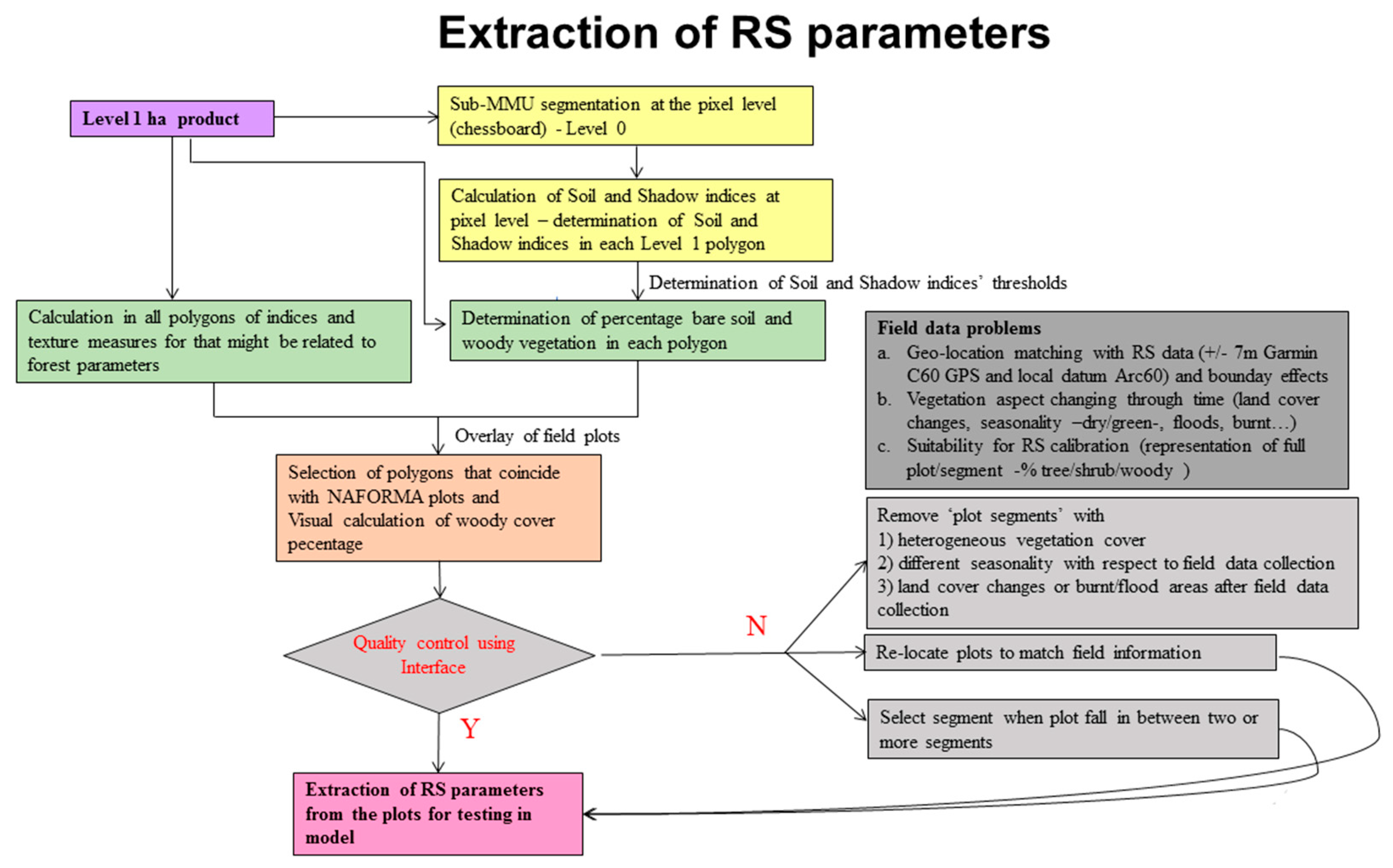
2.5. RapidEye Preprosessing—Image Segmentation to Obtain The MMU

The UNFCC, at its 7th Convention of the Parties (COP), proposed that countries should choose an MMU no greater than 1 ha [70]. For its submission to the UNFCCC, Tanzania used a 0.5 ha MMU [71].

Image segmentation was chosen to map landscape units at a cartographic MMU corresponding as closely as possible to that set by the national authority responsible for forests (the Tanzania Forest Service) and international guidelines. Almost all national forest definitions are based on tree height and tree cover with a minimum mapping unit. Remote sensing data are imaged at the pixel level and so segmentation allows us to cluster pixels of a similar reflectance and texture into objects (vector polygons) that correspond to landscape units (e.g., ‘a forest’) [72]. The segmentation of the image into the objects is achieved through the software package, eCognition [73].

To select the segmentation parameters which determine the aggregation of pixels to objects (or polygons), we effectuated a series of tests changing the shape factor, the compactness, and reflectance weights of the segmentation process executed in the eCognition software package. We found that a high compact value (0.9) provided results that were more in line with traditional photo interpretation results. Results with lower compactness gave us highly fragmented polygons.

The shape factor is the parameter (integer > 1) that controls the size of the objects [74]. The greater the shape factor, the larger the objects. However, the results of the segmentation (i.e., object size) are dependent not only on the shape factor, but on the image itself, i.e., the image contrast, variance and landscape fragmentation. Therefore, a different value of the shape factor parameter may be required to obtain objects of the same size on different images. In conjunction with the FAO, the JRC developed an iterative routine applied to each image to create initial, small, landscape units, and then in a stepwise process, increased these units until the mean object area of each of the image corresponded to the MMU (Figure 3). Objects smaller than the MMU were then dissolved and added to the adjacent object with the closest spectral signature [72]. As the mean object area must be calculated only on land cover features, objects corresponding to clouds and cloud shadows had to be detected, masked out, and omitted from the routine. An example of the increasing shape factor iteration is given in the Supplementary Materials Figure S3 with the final result in Figure S4.

The texture of the image’s reflectance can be an effective parameter for measuring AGB [26,27,75]. To have a consistent measure of texture, the scale of analysis (kernel) needs to be large enough to cover the variation in the target landcover with respect to the resolution of the satellite data. At fine spatial scales (e.g., 1 m), the texture of tree crowns shows high variance. This variation remains high until the unit of observation, i.e., the kernel, is larger than a single tree. We carried out a series of tests extracting texture measures from the RapidEye data using a set of incrementally increasing circular units in homogeneous landscapes from 0.25 ha to 6.25 ha to find a MMU that gave stable (i.e., invariant) results (Supplementary Materials Figure S2). Some texture measurements were highly sensitive to the size of the image object, but stabilized at 1 ha. This was then used as the MMU for our objects. One hectare is larger than the final national specification (0.5 ha), but is in line with international guidelines.

2.6. Cloud and Cloud Shadow Masking

The RapidEye data exhibited two artefacts that needed to be addressed: (i) Cloud and cloud shadow displayed a locational shift of several pixels between image bands, (ii) the sun azimuth angle, which is used in classification software for detecting cloud shadow, was missing in the metadata.

The locational shift (i) between bands is as a result of the push-broom design of the RapidEye sensor, which means that different spectral channels are acquired at slightly different times. This effect is combined with a parallax effect, which depends on the height of the cloud in the individual images [76]. We therefore used an incremental approach whereby an initial (high) reflectance threshold of 50% was applied to detect core cloud areas in each band [77], creating ‘core cloud objects’. These objects were then merged together and then a lower (10%) threshold was applied only to those areas adjacent to the core areas (i.e., edge of cloud). This has the effect of expanding the area classified as cloud.

To address (ii) that of the missing the sun azimuth angle, an interface was developed to visually estimate the sun azimuth angle. An operator used the position of clouds and their respective shadows to provide an angle for the missing value to replace the missing metadata.

2.7. Extraction of Remote Sensing Parameters for Developing Models for AGB

After cloud and cloud shadow masking, the segmentation iteration loop, as described in Section 2.5, was run to obtain image objects at the MMU (1 ha) for all images. A set remote sensing parameters were then extracted from the level 1 ha objects corresponding (spatially) to the field data plots. These parameters were then used as the basis for generating a model for relating AGB to remotely sensed data (Figure 4).

The parameters fall into five categories: Simple reflectance means and standard deviations for the objects; derived vegetation indices designed to highlight vegetation characteristics, advanced texture measures based on Grey Level Co-occurrence Matrices (GLCM) [78], and a categorical class giving the percentages of the polygon belonging either to bare soil, grasslands, or woody vegetation.

Spectral indices have been used for detecting vegetation and more specifically forest parameters in a number of studies [79,80]. The shortwave infrared bands (1.6 and 2.7 μm) are found to be highly correlated with forest parameters and canopy cover [52]. Unfortunately, these bands are absent from the RapidEye sensor. Indices, such as the shadow index, have also been used for forest applications [81,82]. Improvements in assessing AGB have been achieved using temporal series to monitor phenological changes [83], however, in our study, we were limited to single data imagery.

As satellite data of finer spatial resolution have become more readily available, the use of the texture measures has become more common (e.g., [84]). The number of texture indices available is extensive (200 are available in the image processing software, eCognition). Each measure (column 1 of Table 2) can be assessed in 5 different directions for each individual band or for all bands combined. Since these indices are computationally time consuming, we used pairwise correlation tests on the parameters to identify those indices that were highly inter-correlated (see correlation matrix in the Supplementary Materials Figure S5). As a result, we reduced the number of potential texture indices to 25.

For the percentages of bare soil, woody vegetation, and photosynthetically active non-woody vegetation, we used the Shadow Index (SI), the Bare Soil Index (BSI) [85], and the Modified Chlorophyll Absorption Ratio Index (MCARI) [86]. To restrict our final models to ‘woody’ vegetation, we produced a classification of each of the RapidEye images based on a decision tree approach [77], which assigns each object to either forest, shrub, or non-forest. The data extraction processing chain (Figure 4) was implemented in eCognition (the rule set is available both as text and an eCognition dcp file in the Supplementary Materials). The list of reflectance and texture measures extracted from the RapidEye objects is shown in

Table 3. List of reflectance and texture measures extracted from the RapidEye objects.

Single Band Reflectance of Objects	Equation	Acronym
Mean bands 1 to 5	BLUE, GREEN, RED, REdge, NIR	R1–R5
Standard deviation bands 1 to 5		SD1–SD5
Simple Ratios
Ratio of mean to standard deviation for all bands	[Mean band #]/[SD band #]	e.g., R1SD1
Standard deviation. ratios	[SD band #]/[SD band #]	e.g., SD1SD2
Red Vegetation Index	NIR/RED	RVI
Green Vegetation Index	NIR/GREEN	GVI
Green Red Vegetation Index	GREEN/RED	GRVI
Other Indices
Normalised Difference Vegetation Index [87]	(NIR − RED)/(NIR + RED)	NDVI
Enhanced Vegetation Index [88]	2.5 × ((NIR − RED))/((NIR + 6 × RED − 7.5 × BLUE + 1))	EVI
Soil Adjusted Vegetation Index [89]	(NIR − RED)/((NIR + RED + L)) × (1 + L)	SAVI
Shadow Index [85]	((1 − BLUE) × (1 − GREEN) × (1 − RED))0.33	Shadow_Index
Modified Transverse Vegetation Index [86]	(1.5 × (1.2 × ([R5] − [R2]) − 2.5 × ([R3] − [R2])))/((2 × [R5] + 1)^2 − (6 × [R5] − 5 × ([R3])^0.5) − 0.5)^0.5	MTVI
Modified Chlorophyll Absorption Reflectance Index [90]	(([NIR] − [RED]) − 0.2 × ([NIR] − [GREEN])) × ([NIR]/[RED])	MCARI
Bare Soil Index	((([NIR] + [RED]) − ([REdge] + [BLUE]))/(([NIR] + [RED]) + ([REdge] + [BLUE]))) + 1	Bare_soil
Shadow to Soil Ratio	ShadowIndex/Bare_Soil	Shadsoil
GLCM Texture Features	(1) In all directions, 0°, 45°, 90°, 135°
	(2) For combined and for individual bands
Homogeneity	See Haralick [91]	GCLM_Hom
Contrast		GCLM_Con
Dissimilarity		GCLM_Diss
Angular 2nd moment		GCLM_Ang2
Entropy		GCLM_Entro
Mean		GCLM_Mean
Variance		GCLM_StdDev
Correlation		GCLM_Corr
Object Proportions
Bare Soil	Percentage classed as bare soil	Rel_soil
Shadow	Percentage classed as woody	Rel_shad

.

2.8. Reviewing the Field Plot Data with Respect to the Rapideye Data

To assess the compatibility between field data and image data, we developed an interface displaying the image data, the plot location, and the plot information (see Supplementary Materials Figure S6). A number of problems came into evidence during this review. These related to spatial mismatches, temporal mismatches between image acquisition and field visits, and the impact of mixed land cover within the sample sites.

Specifically:

-

The field data (15 m circle plots—circa 700 m²) cover 27 RapidEye pixels. However, the precision of the plot geolocation taken in the field (Garmin C60) had limited accuracy (+/−7 m). There are also known problems in changing between the Arc60 datum of topographic maps of East Africa used in the field survey, and that of the satellite reference datum, UTM-WGS84 [92];

-

there were a number of discrepancies in the geolocation of various RapidEye scenes, which after the review, were addressed by shifting images to a reference data base of Landsat scenes. Over 50 sample site images were shifted by up to 12 pixels, 30 in the X direction and 41 in the Y direction;

-

temporal differences; the field data collection took place over three years; satellite data were only available for one of these years. On average, the difference between field data collection and satellite image acquisition was 10 months (see Supplementary Materials Figure S1), with most of the field data collected after the image acquisition;

-

data collected in the field gave no systematic estimation of the respective cover of trees, shrubs, or other land cover classes, despite being foreseen in the original protocol. On a number of occasions, when given, the canopy cover did not correspond to that seen from the satellite image—perhaps due to problems of geolocation between the data sets, or differences in the time between the field visit and the image acquisition. Also, canopy density is known to be difficult to measure with accuracy from the ground [8];

-

the land cover classification given to the field teams was not adapted to providing adequate field data for calibrating remote sensing data. The vast majority of plots were classified as ‘woodland’, without further elaboration;

-

even if the land cover has not changed throughout the year, its condition does, especially in the tropics, predominantly due to seasonality. It may be in a lush green phase, drying out, exceptionally dry, burnt, or flooded. All these present different spectral signatures for the same land cover. We removed 33 plots that were burnt, 9 that were flooded, and 13 that had cloud or cloud shadow; and

-

finally, we found that the field plot was not always representative of the 1 ha image object on the remote sensing data.

2.9. Models for Predicting Above Ground Biomass

We tested four predictive models to relate the remotely sensed parameters to AGB and evaluated their accuracies. Two models using inferential statistics (i.e., a generalised linear model and a generalised exponential model) and two machine learning models (i.e., a random forest model and a support vector machine (SVM) model). The predictors of the models are image bands, their textures, and spectral indices, while the response variable is the AGB. A scatterplot of each input variable (predictors in the y axis) and biomass is shown in the Supplementary Materials Figure S7.

In the generalised linear model, the dependent variables are assumed to be a linear function of several independent variables, where each of them has a weight (i.e., a regression coefficient). Generalised linear models require a linear relation between predictors and response variables.

Allometric equations relating tree height and basal area to volume, hence calculating AGB, are generally non-linear [11]. We therefore employed a logarithmic transformation to the dependent variables, which is a generalised exponential regression.

Random forest (RF) [93] is an ensemble method that builds several decision trees (weak learners) and outputs the mean prediction of the individual decision tree models. The improved RF strategy alleviates the often reported overfitting problem of simple trees. The decorrelation of the decision trees is achieved through the random selection of the input explanatory variables [94] by bootstrap methods. In this case, 63% of the data is used for training (in-bag data) and the remaining 37% (out-of-bag data) for validation. The choice of random forest was mainly motivated by: (i) RF runs efficiently on large databases (i.e., it is relatively fast to build and even faster to predict), (ii) RF is resistant to outliers and over-training, (iii) RF does not require cross-validation for model selection, (iv) RF provides further information about the most relevant variables inputted in the model, and (v) RF is computationally parallelizable. In a decision tree, an input is entered at the top and as it moves down the decision tree the data gets binned into smaller and smaller sets. The main principle behind ensemble methods is that a group of “weak learners” can come together to form a “strong learner”, for details see [93]. Two parameters are important in the RF algorithm: (i) The number of decision trees used in the forest (ntree) and (ii) the number of random variables used in each decision tree (mtry). In our RF model, we have 500 decision trees (i.e., ntree = 500) and the default mtry value (i.e., mtry = 9). To find the correct ntree number, we built RF models with different ntree values, recorded the error, and computed the number of decision trees needed to reach the minimum error estimate. RF provides the percentage of variance explained and the most relevant input variables in the model. For reproducibility, we used a fixed random number parameter, which forces the generator to give the same random numbers in the random forest function. Since random forest performances generally increase as the size of training data increases, we trained the final model with the entire ground truth dataset.

Random forest is also able to provide information about the importance of the predictors. Specifically, the mean decrease accuracy (“%IncMSE”) (Figure 5) has been used as a measure of variable importance. The %IncMSE quantifies by how much the removal of each variable reduces the accuracy of the model. The higher the %IncMSE is, the more important the variable. We ran random forest 100 times to find a robust estimate of these predictors, with the average values and the quartile distributions of the 20 most relevant predictors shown in Figure 5. The Shadow Index was found to be the most important variable. R2SD2 (that is the ratio of band 2 reflectance to its standard deviation) and MCARI are also able to influence AGB variability. Other predictors are ranked lower in their relative variable importance. The main limitation of the random forest model is the lack of capacity to predict beyond the range of the response values in the training data.

The support vector machines (SVM) are supervised learning methods used for regression tasks that originated from statistical learning theory [95]. SVM methods perform a linear regression in a high dimension using kernels. This allows it to capture nonlinear tendencies in the original input data. SVM has some parameters that need to be selected (i.e., the kernel) and tuned (i.e., cost and gamma) to obtain a better performance. Among all the kernels available in the literature, we chose the radial basis function (RBF) kernel, due to theoretical and computational convenience. In order to optimise the SVM, we have tested several different cost and gamma values, and returned the one which minimizes the mean squared error for a 10-fold cross validation. Specifically, the optimal values were found as 10 and 0.5 for the cost and gamma parameters, respectively.

The ground truth dataset is the national field data set collected by NAFORMA that consists of 512 points where we have AGB information (circa 500 other points were excluded due to very low or zero biomass, detected on the basis of the decision tree classifier—Section 2.7). The ground truth dataset was split, 85% into a training dataset (435 points) and 15% into a validation dataset (77 points). Random forest already separates partial data for an internal validation (i.e., 63% of the data is used for training and 37% for validation as discussed in Section 2.9), but to compare results with other models, it has been trained and validated with the same validation dataset as for the other models. This scheme ensures: (i) That identical datasets are used for training and (ii) an independent validation with a dataset not included in the training phase.

Once we obtained the best model for AGB, we created the final model using all of the ground truth dataset (for further details see next section). The final model was then applied to all the image objects pre-classified as ‘woody’ in the full Remote Sensing data set, so as to obtain AGB estimates for each of the remote sensing sample sites.

Four statistical indicators were used to evaluate the performances of the models: (i) Root mean square error (RMSE); (ii) mean absolute error (MAE); (iii) relative root mean square error (relRMSE); and (iv) the coefficient of determination (R²). Note that results of models refer only to the validation dataset, however, the performance of the model with the training dataset is shown in the Supplementary Materials Figure S8.

2.10. Interpolating the Results to the National Level

To obtain the country level estimates, we interpolate by direct expansion to using the Direct Expansion Estimator. The application of the direct expansion method has been used in various studies [52].

$$AGB=D\times \overline{y}$$

(3)

where D is the total study area and $\overline{y}$ is the average AGB ha⁻¹ of the sample areas.

2.11. The Relative Efficiency to Measure the Improvement in Precision Brought by the Remote Sensing Data

We calculated REff, the relative efficiency (i.e., the ratio of the variance of the estimates for the AGB calculated from the RapdiEye data combined with field data (VAR_REFD) to the variance of the AGB from the field plots alone (VAR_FD). This measures the improvement in precision (as opposed to accuracy) that the introduction of the remote sensing data brings [96]. In theory, a relative efficiency of X would mean that the improvement brought about by the introduction of the remotely sensed data could be achieved by using X times as many field plots [10].

REff = VAR_REFD/VAR_FD

(4)

An estimate [52] can be made with:

$$\mathrm{REff}=\frac{1}{1-R^2}$$

(5)

where R² is the square of the Pearson coefficient of correlation between the remote sensing data and the field data.

3. Results

3.1. Model Results

Table 4. Statistical indicators of modelled data versus observed AGB.

Model	RMSE	MAE	R2	relRMSE
Generalized Exponential Regression	44.55	36.44	0.32	21%
Generalized Linear Regression	41.81	35.07	0.39	20%
Random Forest	30.00	21.64	0.69	14%
SVM	39.08	29.76	0.42	19%

summarizes these main statistical indicators, with scatterplots of the difference between the observed and modelled AGB shown in Figure 6. All performance measures (i.e., RMSE, MAE, relRMSE, R², and observed vs. modelled scatterplots) were assessed using only the validation dataset, with random forest exhibiting the best correlation (R² = 0.69).

The RMSE of the random forest model is ~30, with an MAE of ~20 and an relRMSE of 15%. The performance of SVM is less satisfactory: RMSE is ~40, MAE is ~30, and relative RMSE is ~40%. As expected, the four methods presented a gain in performance on the training dataset, showing the RF with very high accuracies (i.e., RMSE~15, R² = 0.93), while the exponential and linear regression methods still presented poor (biased) estimates of AGB (see Supplementary Materials Figure S8). However, all four methods produce biased results, overestimating low AGB and underestimating AGB, as indicated by the slopes’ deviation from the 1:1 line.

3.2. Analysis at the National Level and by Ecoregion

For our sample sites, covering 2.3% of the country, we find an average of 22.1 tons per ha of above ground biomass (AGB). This is only for those landscape units that are classed as being ‘woody biomass’. Using the areas provided by NAFORMA for forests and woodlands (54,534,500 ha), this results in a total of 602.4 MtC for the country and compared to the estimate from the field plots of 624.9 MtC, a difference of 4%. The standard deviation is high—25%, however, this is not unusual, as land cover is not generally distributed in a regular manner, especially in Tanzania, which exhibits land covers of highly different levels of biomass.

Using the location of the individual sample sites, we calculated the average AGB for the respective ecoregions (

Table 5. Estimates of average AGB (t ha⁻¹) by White ecoregion. *, Refers to the number of RapidEye sites in each ecoregion.

	Afromontane	Zanzibar-Inhambane	Somalia-Masai	Zambezian	Lake Victoria
Area (km2)	43,500	77,100	238,965	502,052	40,300
Count *	5	6	19	41	4
Minimum	17.3	15.1	9.8	11.6	17.8
Maximum	27.7	30.4	22.4	34.3	25.9
Mean	20.9	21.5	16.7	25.2	22.3
SD	4.9	5.6	4.1	4.6	3.3

). Due to the limited number of samples in the other ecoregions, the informative results are for the Somalia-Masai and Zambezian regions.

3.3. Relative Efficiency

The relative efficiency (REff) is calculated using Equation (5), which gives a REff of 3.2. The introduction of the remote sensing data can therefore reduce the field data collection by three, obtaining the same precision.

This result helps in answering one of the main questions of the study: “How much RapidEye can improve the precision of field-based inventory estimates of above-ground biomass in forests and woodlands of Tanzania?”

4. Discussion

A key point that this paper wishes to address is how to improve the link between remote sensing parameters and data collected in the field.

4.1. Practical and Operational Consderations to Imprvve AGB Estimates from RapidEye Data

In preparing data for testing models to relate remote sensing parameters to field data (AGB), we found that a major effort was required in ‘cleaning’ the field data. By ‘cleaning’ we mean removing those aspects of the field data that reduce their potential to calibrate remote sensing data for biomass estimation. The country wide RS data acquired under the GMES initiative was restricted to 2010–2011, whereas the field data were collected over a period of three years. Hence a temporal difference often occurs between a specific image and the corresponding field measurement. However, few plots would have undergone a change during this time lapse. To avoid cloud contamination, most images come from the dry season. At this time, the vegetation is senescent, with trees and shrubs losing their leaves. In this situation, the differences in reflectance between grasslands, shrub and tree savannah, and open woodlands is reduced.

4.1.1. Co-Location of the Data Sets

The site visits for field data plots were organized without using remote sensing imagery. Field teams, using the national topographic maps (in Arc60 datum), navigated to the pre-selected sites. Such field visits should be supported by cartographic and digital extracts of the field locations. Both high cost (high precision GPS with inbuilt satellite and/or map visualisation) and low cost (smart phone/pad and PDF maps) exist to facilitate both navigation and on site location. When local datum are used, so as relate to the national mapping datum, dual GPS locations with WGD 1984 should be employed.

4.1.2. Data Collected

The data collected for the national assessment were suited for the statistical assessment of biomass and for other parameters. However, we found that they were not specific enough to easily correlate them to the satellite data. Optical satellite data record reflectance values within the plot that can be related to the vegetation canopy cover, distribution condition (dry/green/burnt/flooded), and structure. The field data collected need to correspond to these vegetation parameters, which should be recorded and mapped on site during the survey with the aid of an orthomap produced from the remote sensing data to be used in calibration.

4.1.3. Data Cleaning

The inclusion of non-woody, low biomass sites was found to introduce high variance in the spectral signatures for similar values of AGB. These sites have a high variation in land cover and land cover condition. They include barren surfaces, agriculture exploitations, grasslands, and park savannah, each of which manifested different states—burnt, flooded, green flush, senescence, bare soil. We therefore removed them from the data set, reducing the available points from circa 1000 to circa 500.

4.1.4. Spectral Signatures

The reflectance of forest canopy depends on a number of factors, structure, or row orientation (for young artificial forests), optical properties of the background (soil and understory), and canopy geometry [97]. The Shadow Index was found to be the most relevant parameter related to AGB, followed by texture measures. The value of the Shadow Index increases as the forest density increases, hence it is appropriate for relating to woody biomass.

Mature, natural forest stands tend to have more heterogeneous surfaces than non-forest and young regrowth, creating more shadows. The shortwave (1.6 µm and 2.7 µm) infrared bands (SWIR) have been shown to be highly successful in mapping forests [97]. This is mainly because at these wavelengths, there is very low diffuse light, hence shadows are more contrasted. In the absence of SWIR bands on the RapidEye sensor, we used the shadow index as defined by Rikimaru et al. (2002) [58], which uses the visible bands only. Similarly, texture measures, at finer spatial resolutions, differentiate between heterogeneous and homogenous surfaces (Table 3).

4.1.5. Ancillary Data

The parameters entered into the model came exclusively from the single date RapidEye data. While these (RapidEye) are superior in terms of resolution, they are limited for temporal analysis. With the arrival of the Sentinel 2a & 2b sensors, 10 m resolution data are now available at a 5 day frequency. Simulation of this scenario with the SPOT4take5 program [98] has already shown that differences in forest canopy cover (and as a result AGB) can be determined [99].

4.2. Reviewing the Results

4.2.1. Estimation by Ecozone

The Somalia-Masai shows a significantly lower biomass than the Zambezian region (Table 5) as expected, the former is dominated by shrub formations, the latter by woodlands. The other zones are too small to consider using this methodology due to the small number of RapidEye images available in each zone. The Zanzibar-Inhambane, home of the Coastal forests, should have a high average AGB, however, it is these forests that have been depleted most by the impact of exploitation by residents of Dares Salaam and Morogoro [100].

4.2.2. Relative Efficiency

It is difficult to quantify the potential financial savings the inclusion of remote sensing data would bring to the project without knowing the direct costs of the field survey. In the NAFORMA project, the total spent on salaries for the field survey component alone was circa $5 million [63]. However, this includes household surveys (n = 3500) and soil data collections (n = 4000). The costs of overheads, vehicles, and fuel would need to be added. In any case, a relative efficiency of over three indicates that when combined with remote sensing data, the field component could be more than halved to obtain the same precision. The cost of RapidEye data at the time was around $1 per square kilometre, giving a commercial cost of just over $30,000 for the satellite data used in this study. Full country coverage by RapidEye would be around $1 million. Such a coverage would also provide a wall-to-wall map of biomass, which could allow for the estimation of biomass in small ecozones described above.

4.2.3. Model Results

The final model has to cover the full variation in vegetation types and conditions across Tanzania. Clearly, studies on small areas [45], single ecosystems [39], or a mono-species plantation [46] will provide better results, however, these are not comparable to a country wide assessment.

It should be noted that two field plots may have the same AGB, but with totally different characteristics, in terms of vegetation type, cover, and condition. We can imagine a plot with one tree surrounded by grass having the same AGB as a plot fully covered by shrub. This is where the strength of random forest lies, applying a decision tree to associate different input parameters (in this case RS variables) to the same class.

Compared with the other methods available, random forest considerably reduces the dispersion of residuals (e.g., RMSE) and increases the model fit (R²). Despite this improvement in accuracy and precision, the AGB estimate presents a reduced range (40–150 t ha⁻¹ in the case of random forest), which is much lower than the response values in the training data (in the range of 10–200 t ha⁻¹). Specifically, the statistics by the biomass range show that RF tends to overestimate biomass in the range of 0–40 t ha⁻¹ and underestimates it at higher values (i.e., above 150 t ha⁻¹).

Note that this behavior is present for all the four models and is minimized for RF. This behaviour has been observed in many other AGB products [101]. A solution to this would be to compute AGB error statistics for biomass ranges (i.e., 0–50 t ha⁻¹, 50–100 t ha⁻¹). It also has to be remembered that the biomass estimates themselves are interpolated from field measures using allometric equations, which in themselves may have bias for certain ranges of AGB [62].

The AGB overestimation at low biomass and underestimation at high biomass is still an open issue, which has been widely reported in the literature using either optical or radar data (e.g., [102]). Although the presence of a bias can be regarded as a main drawback of such maps, this caveat does not mean that the model result is without merit, as all models are affected by various limitations, and their identification allows a proper use of the outputs. For example, if the map accuracy is not sufficient for certain applications (e.g., local level management), other applications (e.g., stratification, regional analysis) can benefit from knowing the spatial distribution of biomass in relative terms. In any case, quantile analysis on the results of RF regression (Supplementary Materials Figure S9) shows that RF is able to discriminate four main levels of AGB with a relatively good accuracy (e.g., 70% and almost 80% for low and high values, respectively) and the bias in the extremes is not so important.

Underestimation of high biomass values may be due to the following reasons:

(i)

The limited sensitivity of satellite sensors to variations in canopy height and tree diameter in dense forests. Specifically, optical sensors’ radiometers (such as RapidEye) tend to saturate at high biomass in dense forest where there is a weak reflectance-biomass relationship, e.g., [103]. For this reason, the combined use optical data in combination with SAR and LiDAR data would improve results as shown in [104,105];

(ii)

we were limited to the use of single date imagery with most of the images acquired in the dry season when many seasonal forests have lost their leaves and are spectrally similar to low biomass grasslands; and

(iii)

RF is trained on a dataset where high biomass values represent the tail of the frequency distribution and therefore its performance decreases as the biomass increases.

With regards to low biomass values, there could be two explanations: (i) Confusion between understory vegetation and forest canopy where shrubs might be confused with the canopy thus overestimating AGB; and (ii) tree savanna, isolated trees may tend to have a larger canopy, which is relatively similar (as seen from satellite) to that of a denser forest.

The use of diverse data sources may overcome this problem: Combining space borne SAR (e.g., ALOS PALSAR 2, Envisat ASAR, Sentinel-1), optical (e.g., Landsat 7 & 8, Sentinel-2), LiDAR (ICESAT), and auxiliary datasets with multiple estimation procedures as executed by Avitabile et al. [106].

Our work demonstrated that forest services face major hurdles when trying to integrate remote sensing data into a national inventory. These hurdles include obtaining cloud free data for all reference (field) measurements at dates as close to the data collection campaign as possible; ensuring a good geolocation of the two data sets; and having an adequate representation of the distribution of the biomass levels across the full country. We provide potential users with techniques to cope with these problems and show that optical data of finer spatial resolution, in this case 5 m resolution, can be used to obtain biomass estimates at a national level, albeit, with some bias. The arrival of the freely available Sentinel-2 satellite data (although at 10 m resolution) provides an opportunity for more frequent wall-to-wall national coverage. Since 2016, wide area coverage has been available from the commercial 3 m spatial resolution PlanetScope set of satellites [107].

In our study, we were limited by the sampling scheme and the acquisition dates of the available RapidEye data. The scheme, a regular systematic grid, was devised for a continental scale forest change estimates. A more appropriate approach would be to use a stratified random scheme with more (smaller) samples (e.g., [50]) so as to better capture the variance of the biomass across the different ecosystems. While the sampling approach is an efficient method for obtaining biomass estimates, is does not provide a wall-to-wall cartographic product, which would be a benefit for forest management planning and provide orthomaps to support the field survey and stratified estimation [108].

5. Conclusions

We found that remote sensing parameters extracted from 5 m resolution satellite data combined with modelling using the random forest algorithm were an effective method for improving the precision of AGB estimates.

The Shadow Index was found to the most relevant parameter related to AGB, followed by texture measures. The use of both vegetation indices and texture data confirms our hypothesis that a combination of different information extracted from the RS data enhances the precision of AGB estimation, but also can increase bias. This is because the relationship between reflectance and AGB over dense forests is affected by the saturation phenomenon. In contrast, textures and non-woody vegetation cover information (i.e., shadow index) might be more sensitive to canopy architecture and structure. As expected, the high performances of random forest are more evident when the response variables are a result of non-linear and complex interactions between multiple predictors, as has been demonstrated in numerous previous studies. The RF was shown to be quite robust for including a large number of heterogeneous input variables. Also, many predictors of AGB are highly inter-correlated and RF handles both these and redundant variables well.

In terms of supporting REDD+ initiatives, this work demonstrates that nationwide AGB inventories can be carried out in a more rapid and cost effective way by combining 5 m resolution optical satellite data with field plots.

The codes and data used for this study have been made permanently and publicly available in the Supplementary Materials so that results are entirely reproducible.

References

1. Van der Werf, G.R.; Morton, D.C.; DeFries, R.S.; Olivier, J.G.J.; Kasibhatla, P.S.; Jackson, R.B.; Collatz, G.J.; Randerson, J.T. CO2 emissions from forest loss. Nat. Geosci. 2009, 2, 737–738. [Google Scholar] [CrossRef]
2. UNFCCCC. Report of the Conference of the Parties on Its Nineteenth Session, Held in Warsaw from 11 to 23 November 2013. Part One: Proceedings; United Nations Framework Convention on Climate Change: Bonn, Germany, 2014. [Google Scholar]
3. IPCC. Revised 1996 IPCC Guidelines for National Greenhouse Gas Inventories; IPCC: Geneva, Switzerland, 1996. [Google Scholar]
4. IPCC. Good Practice Guidance for Land Use, Land-Use Change and Forestry (GPG-LULUCF); IPCC: Geneva, Switzerland, 2003. [Google Scholar]
5. GOFC-GOLD; Achard, F.; Boschetti, L.; Brown, S.; Brady, M.; DeFries, R.; Grassi, G.; Herold, M.; Mollicone, D.; Pandey, D.; et al. A Sourcebook of Methods and Procedures for Monitoring and Reporting Anthropogenic Greenhouse Gas Emissions and Removals Associated with Deforestation, Gains and Losses of Carbon Stocks in Forests Remaining Forests, and Forestation. Available online: https://www.researchgate.net/publication/283417201_A_sourcebook_of_methods_and_procedures_for_monitoring_and_reporting_anthropogenic_greenhouse_gas_emissions_and_removals_associated_with_deforestation_gains_and_losses_of_carbon_stocks_in_forests_remai (accessed on 28 January 2019).
6. Herold, M.; Román-Cuesta, R.M.; Mollicone, D.; Hirata, Y.; Van Laake, P.; Asner, G.P.; Souza, C.; Skutsch, M.; Avitabile, V.; MacDicken, K. Options for monitoring and estimating historical carbon emissions from forest degradation in the context of REDD+. Carbon Balance Manag. 2011, 6, 1–7. [Google Scholar] [CrossRef] [PubMed]
7. Maniatis, D.; Mollicone, D. Options for sampling and stratification for national forest inventories to implement REDD+ under the UNFCCC. Carbon Balance Manag. 2010, 5, 9. [Google Scholar] [CrossRef] [PubMed] [Green Version]
8. Jennings, S.; Brown, N.; Sheil, D. Assessing canopies and understorey illumination: Canopy closure, canopy cover and other measures. Forestry 1999, 72, 60–73. [Google Scholar] [CrossRef]
9. Gonçalves, F.; Treuhaft, R.; Law, B.; Almeida, A.; Walker, W.; Baccini, A.; dos Santos, J.; Graça, P. Estimating Aboveground Biomass in Tropical Forests: Field Methods and Error Analysis for the Calibration of Remote Sensing Observations. Remote Sens. 2017, 9, 47. [Google Scholar] [CrossRef]
10. Hansen, E.; Gobakken, T.; Solberg, S.; Kangas, A.; Ene, L.; Mauya, E.; Næsset, E. Relative Efficiency of ALS and InSAR for Biomass Estimation in a Tanzanian Rainforest. Remote Sens. 2015, 7, 9865–9885. [Google Scholar] [CrossRef] [Green Version]
11. Chave, J.; Andalo, C.; Brown, S.; Cairns, M.A.; Chambers, J.Q.; Eamus, D.; Fölster, H.; Fromard, F.; Higuchi, N.; Kira, T.; et al. Tree allometry and improved estimation of carbon stocks and balance in tropical forests. Oecologia 2005, 145, 87–99. [Google Scholar] [CrossRef]
12. Henry, M.; Picard, N.; Trotta, C.; Manlay, R.J.; Valentini, R.; Bernoux, M.; Saint-André, L. Estimating tree biomass of sub-Saharan African forests: a review of available allometric equations. Silva Fennica 2011, 45, 477–569. [Google Scholar] [CrossRef]
13. Lewis, S.L.; Sonke, B.; Sunderland, T.; Begne, S.K.; Lopez-Gonzalez, G.; van der Heijden, G.M.F.; Phillips, O.L.; Affum-Baffoe, K.; Baker, T.R.; Banin, L.; et al. Above-ground biomass and structure of 260 African tropical forests. Philos. Trans. R. Soc. B Biol. Sci. 2013, 368, 20120295. [Google Scholar] [CrossRef]
14. Feldpausch, T.R.; Banin, L.; Phillips, O.L.; Baker, T.R.; Lewis, S.L.; Quesada, C.A.; Affum-Baffoe, K.; Arets, E.J.M.M.; Berry, N.J.; Bird, M.; et al. Height-diameter allometry of tropical forest trees. Biogeosciences 2011, 8, 1081–1106. [Google Scholar] [CrossRef] [Green Version]
15. Goetz, S.; Dubayah, R. Advances in remote sensing technology and implications for measuring and monitoring forest carbon stocks and change. Carbon Manag. 2011, 2, 231–244. [Google Scholar] [CrossRef] [Green Version]
16. Timothy, D.; Onisimo, M.; Riyad, I. Quantifying aboveground biomass in African environments: A review of the trade-offs between sensor estimation accuracy and costs. Trop. Ecol. 2016, 57, 393–405. [Google Scholar]
17. Goetz, S.J.; Hansen, M.; Houghton, R.A.; Walker, W.; Laporte, N.; Busch, J. Measurement and monitoring needs, capabilities and potential for addressing reduced emissions from deforestation and forest degradation under REDD+. Environ. Res. Lett. 2015, 10, 123001. [Google Scholar] [CrossRef] [Green Version]
18. Avitabile, V.; Herold, M.; Henry, M.; Schmullius, C. Mapping biomass with remote sensing: A comparison of methods for the case study of Uganda. Carbon Balance Manag. 2011, 6, 7. [Google Scholar] [CrossRef]
19. Baccini, A.; Laporte, N.; Goetz, S.J.; Sun, M.; Dong, H. A first map of tropical Africa’s above-ground biomass derived from satellite imagery. Environ. Res. Lett. 2008, 3, 045011. [Google Scholar] [CrossRef] [Green Version]
20. Hansen, M.C.; Potapov, P.V.; Moore, R.; Hancher, M.; Turubanova, S.A.; Tyukavina, A.; Thau, D.; Stehman, S.V.; Goetz, S.J.; Loveland, T.R.; et al. High-Resolution Global Maps of 21st-Century Forest Cover Change. Science 2013, 342, 850–853. [Google Scholar] [CrossRef]
21. Asner, G.P.; Mascaro, J.; Muller-Landau, H.C.; Vieilledent, G.; Vaudry, R.; Rasamoelina, M.; Hall, J.S.; van Breugel, M. A universal airborne LiDAR approach for tropical forest carbon mapping. Oecologia 2012, 168, 1147–1160. [Google Scholar] [CrossRef] [PubMed]
22. Asner, G.P.; Mascaro, J. Mapping tropical forest carbon: Calibrating plot estimates to a simple LiDAR metric. Remote Sens. Environ. 2014, 140, 614–624. [Google Scholar] [CrossRef]
23. Hajj, M.E.; Baghdadi, N.; Fayad, I.; Vieilledent, G.; Bailly, J.-S.; Minh, D.H.T. Interest of Integrating Spaceborne LiDAR Data to Improve the Estimation of Biomass in High Biomass Forested Areas. Remote Sens. 2017, 9, 213. [Google Scholar] [CrossRef]
24. Nelson, R.; Margolis, H.; Montesano, P.; Sun, G.; Cook, B.; Corp, L.; Andersen, H.-E.; deJong, B.; Pellat, F.P.; Fickel, T.; et al. Lidar-based estimates of aboveground biomass in the continental US and Mexico using ground, airborne, and satellite observations. Remote Sens. Environ. 2017, 188, 127–140. [Google Scholar] [CrossRef] [Green Version]
25. Foody, G.M.; Boyd, D.S.; Cutler, M.E.J. Predictive relations of tropical forest biomass from Landsat TM data and their transferability between regions. Remote Sens. Environ. 2003, 85, 463–474. [Google Scholar] [CrossRef]
26. Ploton, P.; Pélissier, R.; Barbier, N.; Proisy, C.; Ramesh, B.R.; Couteron, P. Canopy Texture Analysis for Large-Scale Assessments of Tropical Forest Stand Structure and Biomass. In Treetops at Risk; Lowman, M., Devy, S., Ganesh, T., Eds.; Springer: New York, NY, USA, 2013; pp. 237–245. ISBN 978-1-4614-7160-8. [Google Scholar]
27. Bastin, J.-F.; Barbier, N.; Couteron, P.; Adams, B.; Shapiro, A.; Bogaert, J.; De Cannière, C. Aboveground biomass mapping of African forest mosaics using canopy texture analysis: Toward a regional approach. Ecol. Appl. 2014, 24, 1984–2001. [Google Scholar] [CrossRef] [PubMed]
28. Ploton, P. Assessing aboveground tropical forest biomass using Google Earth canopy images. Ecol. Appl. 2012, 22, 993–1003. [Google Scholar] [CrossRef]
29. Baynes, J. Assessing forest canopy density in a highly variable landscape using Landsat data and FCD Mapper software. Aust. For. 2004, 67, 247–253. [Google Scholar] [CrossRef]
30. Gonzalez, P.; Asner, G.P.; Battles, J.J.; Lefsky, M.A.; Waring, K.M.; Palace, M. Forest carbon densities and uncertainties from Lidar, QuickBird, and field measurements in California. Remote Sens. Environ. 2010, 114, 1561–1575. [Google Scholar] [CrossRef]
31. Saatchi, S.S.; Harris, N.L.; Brown, S.; Lefsky, M.; Mitchard, E.T.; Salas, W.; Zutta, B.R.; Buermann, W.; Lewis, S.L.; Hagen, S.; et al. Benchmark map of forest carbon stocks in tropical regions across three continents. Proc. Natl. Acad. Sci. USA 2011, 108, 9899–9904. [Google Scholar] [CrossRef] [PubMed] [Green Version]
32. Baccini, A.; Goetz, S.J.; Walker, W.S.; Laporte, N.T.; Sun, M.; Sulla-Menashe, D.; Hackler, J.; Beck, P.S.A.; Dubayah, R.; Friedl, M.A.; et al. Estimated carbon dioxide emissions from tropical deforestation improved by carbon-density maps. Nat. Clim. Chang. 2012, 2, 182–185. [Google Scholar] [CrossRef]
33. Langner, A.; Achard, F.; Grassi, G. Can recent pan-tropical biomass maps be used to derive alternative Tier 1 values for reporting REDD+ activities under UNFCCC? Environ. Res. Lett. 2014, 9, 124008. [Google Scholar] [CrossRef] [Green Version]
34. Potapov, P.; Yaroshenko, A.; Turubanova, S.; Dubinin, M.; Laestadius, L.; Thies, C.; Aksenov, D.; Egorov, A.; Yesipova, Y.; Glushkov, I.; et al. Mapping the World’s Intact Forest Landscapes by Remote Sensing. Ecol. Soc. 2008, 13, 51. [Google Scholar] [CrossRef]
35. Mitchard, E.T.; Saatchi, S.S.; Baccini, A.; Asner, G.P.; Goetz, S.J.; Harris, N.L.; Brown, S. Uncertainty in the spatial distribution of tropical forest biomass: A comparison of pan-tropical maps. Carbon Balance Manag. 2013, 8, 10. [Google Scholar] [CrossRef]
36. Peregon, A.; Yamagata, Y. The use of ALOS/PALSAR backscatter to estimate above-ground forest biomass: A case study in Western Siberia. Remote Sens. Environ. 2013, 137, 139–146. [Google Scholar] [CrossRef]
37. Soja, M.J.; Sandberg, G.; Ulander, L.M.H. Regression-Based Retrieval of Boreal Forest Biomass in Sloping Terrain Using P-Band SAR Backscatter Intensity Data. IEEE Trans. Geosci. Remote Sens. 2013, 51, 2646–2665. [Google Scholar] [CrossRef] [Green Version]
38. Cartus, O.; Kellndorfer, J.; Walker, W.; Franco, C.; Bishop, J.; Santos, L.; Fuentes, J.M.M. A National, Detailed Map of Forest Aboveground Carbon Stocks in Mexico. Remote Sens. 2014, 6, 5559–5588. [Google Scholar] [CrossRef] [Green Version]
39. Pham, T.D.; Yoshino, K.; Bui, D.T. Biomass estimation of Sonneratia caseolaris (L.) Engler at a coastal area of Hai Phong city (Vietnam) using ALOS-2 PALSAR imagery and GIS-based multi-layer perceptron neural networks. GISci. Remote Sens. 2017, 54, 329–353. [Google Scholar] [CrossRef]
40. Le Toan, T.; Quegan, S.; Davidson, M.W.J.; Balzter, H.; Paillou, P.; Papathanassiou, K.; Plummer, S.; Rocca, F.; Saatchi, S.; Shugart, H.; et al. The BIOMASS mission: Mapping global forest biomass to better understand the terrestrial carbon cycle. Remote Sens. Environ. 2011, 115, 2850–2860. [Google Scholar] [CrossRef] [Green Version]
41. Englhart, S.; Keuck, V.; Siegert, F. Aboveground biomass retrieval in tropical forests—The potential of combined X- and L-band SAR data use. Remote Sens. Environ. 2011, 115, 1260–1271. [Google Scholar] [CrossRef]
42. Yu, Y.; Saatchi, S. Sensitivity of L-Band SAR Backscatter to Aboveground Biomass of Global Forests. Remote Sens. 2016, 8, 522. [Google Scholar] [CrossRef]
43. Schlund, M.; Davidson, M.W.J. Aboveground Forest Biomass Estimation Combining L- and P-Band SAR Acquisitions. Remote Sens. 2018, 10, 1151. [Google Scholar] [CrossRef]
44. Joshi, N.; Mitchard, E.T.A.; Brolly, M.; Schumacher, J.; Fernández-Landa, A.; Johannsen, V.K.; Marchamalo, M.; Fensholt, R. Understanding ‘saturation’ of radar signals over forests. Sci. Rep. 2017, 7, 3505. [Google Scholar] [CrossRef] [PubMed] [Green Version]
45. Vafaei, S.; Soosani, J.; Adeli, K.; Fadaei, H.; Naghavi, H.; Pham, T.D.; Tien Bui, D. Improving Accuracy Estimation of Forest Aboveground Biomass Based on Incorporation of ALOS-2 PALSAR-2 and Sentinel-2A Imagery and Machine Learning: A Case Study of the Hyrcanian Forest Area (Iran). Remote Sens. 2018, 10, 172. [Google Scholar] [CrossRef]
46. Pham, T.D.; Yoshino, K.; Le, N.N.; Bui, D.T. Estimating aboveground biomass of a mangrove plantation on the Northern coast of Vietnam using machine learning techniques with an integration of ALOS-2 PALSAR-2 and Sentinel-2A data. Int. J. Remote Sens. 2018, 39, 7761–7788. [Google Scholar] [CrossRef]
47. Ho Tong Minh, D.; Ndikumana, E.; Vieilledent, G.; McKey, D.; Baghdadi, N. Potential value of combining ALOS PALSAR and Landsat-derived tree cover data for forest biomass retrieval in Madagascar. Remote Sens. Environ. 2018, 213, 206–214. [Google Scholar] [CrossRef]
48. Deng, S.; Katoh, M.; Guan, Q.; Yin, N.; Li, M. Estimating Forest Aboveground Biomass by Combining ALOS PALSAR and WorldView-2 Data: A Case Study at Purple Mountain National Park, Nanjing, China. Remote Sens. 2014, 6, 7878–7910. [Google Scholar] [CrossRef] [Green Version]
49. Hame, T.; Rauste, Y.; Antropov, O.; Ahola, H.A.; Kilpi, J. Improved Mapping of Tropical Forests with Optical and SAR Imagery, Part II: Above Ground Biomass Estimation. IEEE J. Sel. Top. Appl. Earth Obs. Remote Sens. 2013, 6, 92–101. [Google Scholar] [CrossRef]
50. Potapov, P.; Hansen, M.C.; Stehman, S.V.; Loveland, T.R.; Pittman, K. Combining MODIS and Landsat imagery to estimate and map boreal forest cover loss. Remote Sens. Environ. 2008, 112, 3708–3719. [Google Scholar] [CrossRef]
51. Köhl, M.; Lister, A.; Scott, C.T.; Baldauf, T.; Plugge, D. Implications of sampling design and sample size for national carbon accounting systems. Carbon Balance Manag. 2011, 6, 10. [Google Scholar] [CrossRef] [PubMed] [Green Version]
52. Gallego, F.J. Remote sensing and land cover area estimation. Int. J. Remote Sens. 2004, 25, 3019–3047. [Google Scholar] [CrossRef]
53. Gong, P.; Marceau, D.J.; Howarth, P.J. A comparison of spatial feature extraction algorithms for land-use classification with SPOT HRV data. Remote Sens. Environ. 1992, 40, 137–151. [Google Scholar] [CrossRef]
54. White, F. The Vegetation of Africa: A Descriptive Memoir to Accompany the UNESCO/AETFAT/UNSO Vegetation Map of Africa; UNESCO: Paris, France, 1983; ISBN 92-3-101955-4. [Google Scholar]
55. MNRT. NAFORMA Main Results; MNRT: Dodoma, Tanzania, 2015.
56. UN-REDD. Draft Action Plan for Implementation of National Strategy for REDD+; UN-REDD: Geneva, Switzerland, 2012. [Google Scholar]
57. UN-REDD. Estimating the Cost Elements of REDD+ in Tanzania; UN-REDD: Geneva, Switzerland, 2012. [Google Scholar]
58. NAFORMA. Field Manual, Biophysical Survey; Ministry of Natural Resources and Tourism, Forestry and Beekeeping Division: Dar es Salaam, Tanzania, 2010.
59. Tomppo, E.; Katila, M.; Peräsaari, J.; Malimbwi, R.; Chamuya, N.; Otieno, J.; Dalsgaard, S.; Leppänen, M. A Report to the Food and Agriculture Organization of the United Nations (FAO) in Support of Sampling Study for National Forestry Resources Monitoring and Assessment (NAFORMA) in Tanzania; Sokoine University of Agriculture: Morogoro, Tanzania, 2010. [Google Scholar]
60. Tomppo, E.; Malimbwi, R.; Katila, M.; Mäkisara, K.; Henttonen, H.M.; Chamuya, N.; Zahabu, E.; Otieno, J. A sampling design for a large area forest inventory: case Tanzania. Can. J. For. Res. 2014, 44, 931–948. [Google Scholar] [CrossRef]
61. Hojas Gascón, L.; Eva, H. Field Guide for Forest Mapping with High Resolution Satellite Data; Publications Office: Luxembourg, 2014; ISBN 978-92-79-44012-0. [Google Scholar]
62. Mascaro, J.; Litton, C.M.; Hughes, R.F.; Uowolo, A.; Schnitzer, S.A. Minimizing Bias in Biomass Allometry: Model Selection and Log-Transformation of Data. Biotropica 2011, 43, 649–653. [Google Scholar] [CrossRef]
63. FAO; JRC; SDSU; UCL. The 2010 Global Forest Resources Assessment Remote Sensing Survey: FRA Working Paper 155; FAO: Rome, Italy, 2009. [Google Scholar]
64. Tyc, G.; Tulip, J.; Schulten, D.; Krischke, M.; Oxfort, M. The RapidEye mission design. Acta Astronaut. 2005, 56, 213–219. [Google Scholar] [CrossRef]
65. Beuchle, R.; Grecchi, R.C.; Shimabukuro, Y.E.; Seliger, R.; Eva, H.D.; Sano, E.; Achard, F. Land cover changes in the Brazilian Cerrado and Caatinga biomes from 1990 to 2010 based on a systematic remote sensing sampling approach. Appl. Geogr. 2015, 58, 116–127. [Google Scholar] [CrossRef]
66. RapidEye. Planet Labs San Francisco Satellite Imagery Product Specifications, version 6.1; RapidEye: Berlin, Germany, 2016. [Google Scholar]
67. Beuchle, R.; Eva, H.D.; Stibig, H.-J.; Bodart, C.; Brink, A.; Mayaux, P.; Johansson, D.; Achard, F.; Belward, A. A satellite data set for tropical forest area change assessment. Int. J. Remote Sens. 2011, 32, 7009–7031. [Google Scholar] [CrossRef]
68. Hojas Gascón, L.; Eva, H.; Laporte, N.; Simonetti, D.; Fritz, S. The Application of Medium-Resolution MERIS Satellite Data for Continental Land-Cover Mapping over South America: Results and Caveats. In Remote Sensing of Land Use and Land Cover: Principles and Applications; CRC Press/Taylor & Francis: Boca Raton, FL, USA, 2012. [Google Scholar]
69. Hansen, M.C.; Roy, D.P.; Lindquist, E.; Adusei, B.; Justice, C.O.; Altstatt, A. A method for integrating MODIS and Landsat data for systematic monitoring of forest cover and change in the Congo Basin. Remote Sens. Environ. 2008, 112, 2495–2513. [Google Scholar] [CrossRef]
70. UNFCCC. Report of the Conference of the Parties on Its Seventh Session, Held at Marrakesh from 29 October to 10 November 2001; United Nations Framework Convention on Climate Change: Bonn, Germany, 2001. [Google Scholar]
71. The United Republic of Tanzania. Tanzania’s Forest Reference Emission Level Submission to the UNFCCC 2016. Available online: https://redd.unfccc.int/files/frel__for__tanzania_december2016_27122016.pdf (accessed on 28 January 2019).
72. Raši, R.; Bodart, C.; Stibig, H.-J.; Eva, H.; Beuchle, R.; Carboni, S.; Simonetti, D.; Achard, F. An automated approach for segmenting and classifying a large sample of multi-date Landsat imagery for pan-tropical forest monitoring. Remote Sens. Environ. 2011, 115, 3659–3669. [Google Scholar] [CrossRef]
73. Flanders, D.; Hall-Beyer, M.; Pereverzoff, J. Preliminary evaluation of eCognition object-based software for cut block delineation and feature extraction. Can. J. Remote Sens. 2003, 29, 441–452. [Google Scholar] [CrossRef]
74. Blaschke, T. Object based image analysis for remote sensing. ISPRS J. Photogramm. Remote Sens. 2010, 65, 2–16. [Google Scholar] [CrossRef] [Green Version]
75. Dube, T.; Mutanga, O. Investigating the robustness of the new Landsat-8 Operational Land Imager derived texture metrics in estimating plantation forest aboveground biomass in resource constrained areas. ISPRS J. Photogramm. Remote Sens. 2015, 108, 12–32. [Google Scholar] [CrossRef]
76. Konstanski, H. Apparent Cloud Shift in RapidEye Image Data; RapidEye: Berlin, Germany, 2012. [Google Scholar]
77. Simonetti, D.; Simonetti, E.; Szantoi, Z.; Lupi, A.; Eva, H.D. First results from the phenology-based synthesis classifier using Landsat 8 imagery. IEEE Geosci. Remote Sens. Lett. 2015, 12, 1496–1500. [Google Scholar] [CrossRef]
78. Haralick, R.M.; Shanmugam, K.; Dinstein, I. Textural features for image classification. IEEE Trans. Syst. Man Cybern. 1973, SMC-3, 610–621. [Google Scholar] [CrossRef]
79. Haboudane, D. Hyperspectral vegetation indices and novel algorithms for predicting green LAI of crop canopies: Modeling and validation in the context of precision agriculture. Remote Sens. Environ. 2004, 90, 337–352. [Google Scholar] [CrossRef]
80. Xue, J.; Su, B. Significant Remote Sensing Vegetation Indices: A Review of Developments and Applications. J. Sens. 2017, 2017, 1353691. [Google Scholar] [CrossRef]
81. Lu, D.; Mausel, P.; Brondízio, E.; Moran, E. Relationships between forest stand parameters and Landsat TM spectral responses in the Brazilian Amazon Basin. For. Ecol. Manag. 2004, 198, 149–167. [Google Scholar] [CrossRef] [Green Version]
82. Lu, D.; Chen, Q.; Wang, G.; Liu, L.; Li, G.; Moran, E. A survey of remote sensing-based aboveground biomass estimation methods in forest ecosystems. Int. J. Digit. Earth 2016, 9, 63–105. [Google Scholar] [CrossRef]
83. Gwenzi, D.; Helmer, E.; Zhu, X.; Lefsky, M.; Marcano-Vega, H. Predictions of Tropical Forest Biomass and Biomass Growth Based on Stand Height or Canopy Area Are Improved by Landsat-Scale Phenology across Puerto Rico and the U.S. Virgin Islands. Remote Sens. 2017, 9, 123. [Google Scholar] [CrossRef]
84. Eckert, S. Improved Forest Biomass and Carbon Estimations Using Texture Measures from WorldView-2 Satellite Data. Remote Sens. 2012, 4, 810–829. [Google Scholar] [CrossRef] [Green Version]
85. Rikimaru, A.; Roy, P.S.; Miyatake, S. Tropical forest cover density mapping. Trop. Ecol. 2002, 43, 39–47. [Google Scholar]
86. Eitel, J.U.H.; Long, D.S.; Gessler, P.E.; Smith, A.M.S. Using in-situ measurements to evaluate the new RapidEye satellite series for prediction of wheat nitrogen status. Int. J. Remote Sens. 2007, 28, 4183–4190. [Google Scholar] [CrossRef]
87. Tucker, C.J.; Pinzon, J.E.; Brown, M.E.; Slayback, D.A.; Pak, E.W.; Mahoney, R.; Vermote, E.F.; El Saleous, N. An extended AVHRR 8-km NDVI dataset compatible with MODIS and SPOT vegetation NDVI data. Int. J. Remote Sens. 2005, 26, 4485–4498. [Google Scholar] [CrossRef]
88. Huete, A.; Didan, K.; Miura, T.; Rodriguez, E.P.; Gao, X.; Ferreira, L.G. Overview of the radiometric and biophysical performance of the MODIS vegetation indices. Remote Sens. Environ. 2002, 83, 195–213. [Google Scholar] [CrossRef]
89. Huete, A. A soil-adjusted vegetation index (SAVI). Remote Sens. Environ. 1988, 25, 295–309. [Google Scholar] [CrossRef]
90. Haboudane, D.; Miller, J.R.; Tremblay, N.; Zarco-Tejada, P.J.; Dextraze, L. Integrated narrow-band vegetation indices for prediction of crop chlorophyll content for application to precision agriculture. Remote Sens. Environ. 2002, 81, 416–426. [Google Scholar] [CrossRef]
91. Haralick, R.M. Statistical and structural approaches to texture. Proc. IEEE 1979, 67, 786–804. [Google Scholar] [CrossRef]
92. Moses, M.; Stevens, T.S.; Bax, G. GIS Data Ineroperability in Uganda. Int. J. Spat. Data Infrastruct. Res. 2012, 7, 488–507. [Google Scholar]
93. Breiman, L. Random Forests. Mach. Learn. 2001, 45, 5–32. [Google Scholar] [CrossRef] [Green Version]
94. Hastie, T.; Tibshirani, R.; Friedman, J. The Elements of Statistical Learning—Data Mining, Inference, and Prediction; Springer Series in Statistics; Springer: New York, NY, USA, 2001; Volume 1. [Google Scholar]
95. Vapnik, V.N. The Nature of Statistical Learning Theory; Springer, Inc.: New York, NY, USA, 1995; ISBN 978-0-387-94559-0. [Google Scholar]
96. Payandeh, B. Relative Efficiency of Two-Dimensional Systematic Sampling. For. Sci. 1970, 16, 271–276. [Google Scholar]
97. Guyot, G.; Guyon, D.; Riom, J. Factors affecting the spectral response of forest canopies: A review. Geocarto Int. 1989, 4, 3–18. [Google Scholar] [CrossRef]
98. Hagolle, O.; Huc, M.; Dedieu, G.; Sylvander, S. SPOT4 (Take 5) Times series over 45 sites to prepare Sentinel-2 applications and methods. In Proceedings of the ESA’s Living Planet Symposium, Edinburgh, UK, 9–13 September 2013; Volume 11. [Google Scholar]
99. Hojas-Gascon, L.; Belward, A.; Eva, H.; Ceccherini, G.; Hagolle, O.; Garcia, J.; Cerutti, P. Potential improvement for forest cover and forest degradation mapping with the forthcoming Sentinel-2 program. ISPRS Int. Arch. Photogramm. Remote Sens. Spat. Inf. Sci. 2015, XL-7/W3, 417–423. [Google Scholar] [CrossRef]
100. Hojas-Gascon, L.; Eva, H.D.; Ehrlich, D.; Pesaresi, M.; Achard, F.; Garcia, J. Urbanization and Forest Degradation in East Africa—A Case Study around Dar es Salaam, Tanzania; IEEE: Piscataway, NJ, USA, 2016; pp. 7293–7295. [Google Scholar]
101. Avitabile, V.; Camia, A. An assessment of forest biomass maps in Europe using harmonized national statistics and inventory plots. For. Ecol. Manag. 2018, 409, 489–498. [Google Scholar] [CrossRef]
102. Gao, Y.; Lu, D.; Li, G.; Wang, G.; Chen, Q.; Liu, L.; Li, D. Comparative Analysis of Modeling Algorithms for Forest Aboveground Biomass Estimation in a Subtropical Region. Remote Sens. 2018, 10, 627. [Google Scholar] [CrossRef]
103. Mutanga, O.; Adam, E.; Cho, M.A. High density biomass estimation for wetland vegetation using WorldView-2 imagery and random forest regression algorithm. Int. J. Appl. Earth Obs. Geoinf. 2012, 18, 399–406. [Google Scholar] [CrossRef]
104. Shao, Z.; Zhang, L. Estimating Forest Aboveground Biomass by Combining Optical and SAR Data: A Case Study in Genhe, Inner Mongolia, China. Sensors 2016, 16, 834. [Google Scholar] [CrossRef] [PubMed]
105. Attarchi, S.; Gloaguen, R. Improving the Estimation of Above Ground Biomass Using Dual Polarimetric PALSAR and ETM+ Data in the Hyrcanian Mountain Forest (Iran). Remote Sens. 2014, 6, 3693–3715. [Google Scholar] [CrossRef] [Green Version]
106. Avitabile, V.; Herold, M.; Heuvelink, G.B.M.; Lewis, S.L.; Phillips, O.L.; Asner, G.P.; Armston, J.; Ashton, P.S.; Banin, L.; Bayol, N.; et al. An integrated pan-tropical biomass map using multiple reference datasets. Glob. Chang. Biol. 2016, 22, 1406–1420. [Google Scholar] [CrossRef] [PubMed] [Green Version]
107. Hoa, N.H. Comparison of various spectral indices for estimating mangrove covers using PlanetScope data: A case study in Xuan Thuy national park, Nam Dinh province. J. For. Sci. Technol. 2017, 5, 74–83. [Google Scholar]
108. McRoberts, R.E.; Holden, G.R.; Nelson, M.D.; Liknes, G.C.; Gormanson, D.D. Using satellite imagery as ancillary data for increasing the precision of estimates for the Forest Inventory and Analysis program of the USDA Forest Service. Can. J. For. Res. 2005, 35, 2968–2980. [Google Scholar] [CrossRef]
109. Guidolavespa. Guidolavespa/Forest v1.0; Zenodo: Geneva, Switzerland, 2018. [Google Scholar]
Figure 1. The ecological zone map of Tanzania [54] with the location of the field plots (not to scale) to coincide with the satelite data. An excert of the points for one cluster overlaid on a RapidEye image is shown to the right.
Forests 10 00107 g001
Figure 2. The RapidEye ABG map (a) for a sample centered on the 9° S 38° E confluence point and (b) the satellite image false colour composite (Shortwave Infrared (SWIR), Near-Infrared (NIR), Red). Cloud and cloud shadow are masked out in the first stages of the pre-processing, then image segments are assigned AGB values using the model developed using random forest.
Forests 10 00107 g002aForests 10 00107 g002b
Figure 3. Processing scheme to obtain 1 ha MMUs.
Forests 10 00107 g003
Figure 4. Data extraction scheme.
Forests 10 00107 g004
Figure 5. Box-plot of the importance of variables for AGB in the final Random forest model, showing the increase in mean standard error (MSE) when removing a variable (y-axis), and their importance on the x-axis. For the sake of simplicity, only the first 12 variables are shown. RXSDX denotes the ratio of the band X reflectance to its standard deviation.
Forests 10 00107 g005
Figure 6. Scatterplot of predicted vs. modelled AGB in tha−1 for the four models using the independent validation dataset. Both circle size and colour refer to the actual AGB. Model performance indicators are also shown in Table 4. The blue line indicates the linear regression between the actual and modelled data and the grey area is the 95% confidence level interval.
Forests 10 00107 g006