Combining a Quantum Cascade Laser Spectrometer with an Automated Closed-Chamber System for δ¹³C Measurements of Forest Soil, Tree Stem and Tree Root CO₂ Fluxes

Abstract

Recent advances in laser spectroscopy have allowed for real-time measurements of the ¹³C/¹²C isotopic ratio in CO₂, thereby providing new ways to investigate carbon cycling in natural ecosystems. In this study, we combined an Aerodyne quantum cascade laser spectrometer for CO₂ isotopes with a LI-COR LI-8100A/8150 automated chamber system to measure the δ¹³C of CO₂ during automated closed-chamber measurements. The isotopic composition of the CO₂ flux was determined for each chamber measurement by applying the Keeling plot method. We found that the δ¹³C measured by the laser spectrometer was influenced by water vapour and CO₂ concentration of the sample air and we developed a method to correct for these effects to yield accurate measurements of δ¹³C. Overall, correcting for the CO₂ concentration increased the δ¹³C determined from the Keeling plots by 3.4‰ compared to 2.1‰ for the water vapour correction. We used the combined system to measure δ¹³C of the CO₂ fluxes automatically every two hours from intact soil, trenched soil, tree stems and coarse roots during a two-month campaign in a Danish beech forest. The mean δ¹³C was −29.8 ± 0.32‰ for the intact soil plots, which was similar to the mean δ¹³C of −29.8 ± 1.2‰ for the trenched soil plots. The lowest δ¹³C was found for the root plots with a mean of −32.6 ± 0.78‰. The mean δ¹³C of the stems was −30.2 ± 0.74‰, similar to the mean δ¹³C of the soil plots. In conclusion, the study showed the potential of using a quantum cascade laser spectrometer to measure δ¹³C of CO₂ during automated closed-chamber measurements, thereby allowing for measurements of isotopic ecosystem CO₂ fluxes at a high temporal resolution. It also highlighted the importance of proper correction for cross-sensitivity with water vapour and CO₂ concentration of the sample air to get accurate measurements of δ¹³C.

1. Introduction

The isotopic composition of carbon in CO₂ of ecosystem fluxes can reveal quantitative information about both physiological processes and carbon cycling [1]. In forests, CO₂ enters the ecosystem via C3 photosynthesis, a process that favours the light isotope ¹²C over the heavy isotope ¹³C in CO₂ [2]. This results in a lower ratio of ¹³C to ¹²C, often expressed by the δ notation as δ¹³C, of ecosystem C than in the atmosphere [3]. The ecosystem ultimately loses C by respiration, where soil respiration (R_soil) accounts for more than half of forest ecosystem respiration [4]. R_soil is traditionally measured as soil CO₂ flux by the closed chamber method, where a chamber is placed on top the soil and the flux is calculated based on the CO₂ concentration increase in the chamber headspace over time [5]. The increase in chamber CO₂ concentration can be measured with online laser-based spectroscopy and automated chamber systems have been constructed that provide measurements of soil CO₂ fluxes at a high temporal resolution [6,7,8,9]. Closed chambers have also been used to yield information about the δ¹³C of R_soil. This requires measuring the change in δ¹³C in the chamber headspace as the CO₂ concentration increases. By fitting a linear equation to the δ¹³C and the reciprocal CO₂ concentration, a so-called Keeling plot, the source δ¹³C of the respired CO₂ can be calculated [10]. In contrast to the measurements of CO₂ concentration, measurements of δ¹³C have traditionally been done by labour-intensive manual field samplings followed by laboratory analysis by isotope-ratio mass spectrometers (IRMS) that provide high precision measurements of δ¹³C but are bulky, unfit for field operation and most often only allow for measurements of discrete samples [11]. A recent, novel alternative to IRMS is the emerging use of laser spectroscopy capable of real-time, fast response measurements of δ¹³C. Laser spectrometers have the advantage of being able to perform high frequency, δ¹³C measurements of a continuous air sample and to be operated under field conditions, similar to infrared gas analysers for CO₂. A few technologies have been developed in recent years for measuring δ¹³C in ecosystems including wavelength-scanned cavity ring-down spectroscopy, tunable diode laser absorption spectroscopy and quantum cascade laser absorption spectroscopy [12,13,14,15,16]. Quantum cascade lasers can operate in the mid-infrared where CO₂ show strong fundamental vibrational bands, thus allowing for high precision measurements [17]. They have successfully been used to measure the isotopic flux of CO₂ at ecosystem scale by eddy covariance [18,19], for tree branch photosynthesis in the field [20] and for field measurement of δ¹³C of R_soil by closed chambers [21]. Although a high accuracy can be achieved, the instruments are found to be highly temperature sensitive, why they need to be placed in a temperature-controlled environment during field application, such as inside a temperature-controlled cabin or box [15,22]. Furthermore, closed path laser spectroscopy has been found to be influenced by changes in water vapour in the sample air, which dilutes the gas of interest and causes pressure line broadening that might act differently on ¹²C and ¹³C, thus affecting the apparent measured δ¹³C [23]. Likewise, concentration dependence might be present, which can cause the measured δ¹³C to be influenced by the absolute concentration of CO₂ in a gas sample [24]. Both the influence of water vapour and the absolute CO₂ concentration dependence are instrument specific and must be determined for each individual instrument. For many purposes, including eddy covariance, the sample air can be dried, which eliminates the effect of water vapour on the measured δ¹³C [19]. Furthermore, the change in CO₂ concentration over time during eddy covariance measurements is relatively small and thus, the concentration dependence may be limited. However, it still needs to be quantified, which has been done by varying the CO₂ concentration in calibration gases while keeping the δ¹³C constant [25,26]. In contrast to eddy covariance, the concentration of both CO₂ and H₂O, as well as δ¹³C may all change significantly during a closed-chamber measurement. In addition, sample air is constantly cycled in a loop between the chamber and the laser spectrometer, which can complicate or make it impossible to dry the air before it enters the laser, without potentially disturbing the chamber headspace environment. Thus, the effect of water vapour on δ¹³C must be quantified. Furthermore, because the δ¹³C of the flux is calculated based on the change in CO₂ concentration and δ¹³C during a measurement, the concentration dependence of δ¹³C in the range of CO₂ concentrations during a measurement must also be correctly quantified to accurately estimate δ¹³C.

In the current study we aimed to (I) combine an Aerodyne quantum cascade laser spectrometer for CO₂ isotopes with an LI-8100A/8150 automated closed-chamber system, (II) deploy the system under field conditions in a forest ecosystem to yield high-frequency measurements of δ¹³C of chamber CO₂ flux measurements from tree stems, tree roots, intact soil and trenched soil and (III) quantify the dependence on measured δ¹³C of water vapour in the sample air and on the varying CO₂ concentrations during chamber measurements to yield accurate δ¹³C measurements.

2. Materials and Methods

2.1. Site Description

Measurements were performed at the Danish Integrated Carbon Observation System Research Infrastructure (ICOS RI) site DK-Sor at 40 meters above sea level (55°29′13″ N, 55°28′45″ E), where tower-based eddy covariance measurements have been made since 1996. A dense forest consisting mostly of European beech (Fagus sylvatica L.) covers the site. The climate is temperate maritime with an annual mean temperature of 8.5 °C and an annual mean precipitation of 564 mm. For a comprehensive description of the site see References [27,28].

2.2. Measurements of Soil, Root and Stem Respiration

Respiration from intact soil, trenched soil, coarse tree roots and tree stems was measured by automated closed-chambers controlled by a LI-8100A Automated Soil CO₂ Flux System connected to a LI-8150 Multiplexer (LI-COR Environmental, Lincoln, NE, USA), which allowed for automated sequential measurements of each of the chambers. Eight 4 L opaque soil chambers each measured soil CO₂ flux at circular soil collars with a diameter of 20 cm that were permanently inserted 4 cm into the soil. The soil collars contained soil and litter but no aboveground plant parts. Three of the soil chambers were 8100-101 Long-Term CO₂ flux chambers and five were 8100-104 Long-Term CO₂ flux chambers (LI-COR Environmental, Lincoln, NE, USA). A trenching was performed on 6 April 2016 to remove the contribution of autotrophic root respiration to the total R_soil from four of the plots. The soil was vertically cut to a depth of 25 cm in a circle around four of the eight soil chambers using a spade. Large roots were cut with a saw. To prevent ingrowth of roots over time, a re-trenching was performed monthly.

Root and stem respiration were measured with two custom-made root chambers and two custom-made stem chambers, respectively, similar to the chambers used in Reference [29]. These chambers did not open between measurements. Instead they were continuously flushed with atmospheric air at a flowrate of 1 L min⁻¹ between measurements, which resulted in ambient atmospheric CO₂ concentration in the chambers. A 10 cm tube, with a filter in the end, was attached to the chamber which acted as a vent to the atmosphere.

The root chambers were made of transparent acrylic glass and were cylindrical in shape with an inner length of 24 cm and an inner diameter of 7 cm, giving a volume of 923 cm³. The chambers were installed in June 2015. For each chamber, a coarse root with a diameter of about 0.5 cm was carefully exposed from a depth of 5–10 cm and rinsed with tap water. The cylinder was made of two halves that allowed the root to be enclosed intact in the chamber. The holes in each end of the cylinder, where the root went through, were sealed with Blu-tack. Following this, the chambers were covered in soil.

The stem chambers were cylindrical in shape and made of opaque polypropylene, with an inner diameter of 15 cm and an inner height of 10 cm, giving a volume of 1757 cm². They were attached to the stem surfaces at a height of 1.3 m by a rubber extrusion with a u-profile that was attached to the chamber and sealed with silicone. Each chamber was held in place on the stem by an adjustable nylon strap.

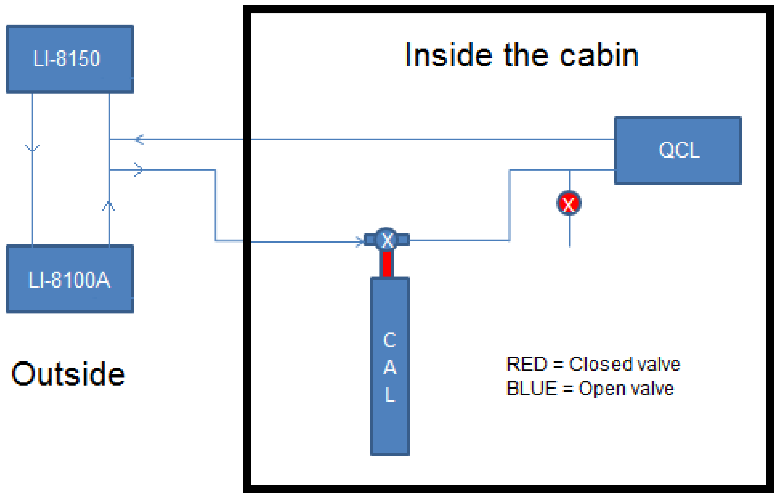
2.3. Combining the Aerodyne Laser Spectrometer with the Li-8100A/8150

We combined the Aerodyne Single Continuous Wave Quantum Cascade Laser Trace Gas Analyzer for CO₂ (δ¹³C and δ¹⁸O) Isotopes (the Mini Laser Trace Gas Monitor, Aerodyne Research Inc. 45 Manning Road Billerica, MA), henceforth called the QCL system, with the LI-COR LI-8100A/8150 system in a parallel loop on the outlet side of the LI-COR system in accordance with Application note 138 [30]. See Figure 1 for setup. Thus, the flow to and from the laser to the LI-8100A/8150 was introduced as a sub loop between the LI-8100A and LI-8150. The nominal flowrate between the LI-8100A and LI-8150 is 1.5 to 1.7 L min⁻¹. The precision of δ¹³C for the QCL system was analysed by the manufacturer. The Allan deviation was 0.062, 0.023 and 0.013‰ for an integration time of 1, 10 and 100 s, respectively. The QCL system was placed in an air-conditioned cabin in the forest where the temperature was kept constant at 20 °C, while the LI-8100A/8150 was placed 10 m outside the cabin. The pressure in the QCL system cell was kept at a pressure below ambient (30 Torr in this case, controlled with a flow controller by the QCL system valve), while the pressure in the LI-8100A/8150 was kept at ambient. A Pfeiffer Vacuum MVP 070-3 pump (Pfeiffer Vacuum GmbH) was connected to the QCL system outlet, which drew air through the QCL system at a flow rate of 1.0 L min⁻¹, that is, slightly lower that the nominal flowrate between the LI-8100A and LI-8150. The lower flow rate to the QCL system is required to prevent “back-looping” of output air from the QCL system into the sub loop, which could cause time-delays in the signal of the QCL system compared to the LI-8100A. The closed-chamber method requires an air-tight system. However, introducing another loop with a heavy pump can potentially cause leaks, thereby biasing the measurements. We therefore tested for leakage in the system by performing a soil chamber measurement where the soil collar was sealed by plastic. The Pfeiffer pump and the QCL system were placed inside the cabin, at a time when the CO₂ concentration in the cabin was high (≈1000 ppm). If the system was leaky, this would result in an increase in CO₂ concentration in the system over time. Following careful fitting and tightening of the tube fittings to and from the pump, a constant ambient CO₂ concentration in the system was achieved, indicating a non-leaky system.

2.4. Measurement Protocol

A measurement campaign using the LI-8100A/8150 system combined with the QCL system was made from 6 June to 15 August 2016. For the campaign, the system was set up in a repeated automated two-hour cycle during which a measurement of each of the intact soil, trenched soil, coarse root and stem chambers was performed, followed by a calibration of the QCL system. The chamber enclosure time was set to 5 min and pre-purge and post-purge were both set to 40 s. During the last 12 min of each two-hour measurement cycle, an automatic calibration of the QCL system was performed. The calibration was performed with a sample of atmospheric air supplied by a 50 L gas cylinder (AGA A/S, Copenhagen, Denmark). A single calibration gas was used, following the recommendation from the QCL system manufacturer. The δ¹³C of the calibration gasses were determined by IRMS (Gasbench in continuous flow mode with a Delta V PLUS, Thermo Scientific, Bremen, Germany) at the Laboratory for Stable Isotopes in soil, plant and air at the University of Copenhagen. Working standards for the IRMS analysis were two mixtures of synthetic air with CO₂ at near ambient concentration certified at −2.7 (‰ vs PDB) and −29.3 (‰ vs PDB), respectively, supplied by Air Liquide (Air Liquide, Høje Taastrup, Denmark). The δ¹³C of the four calibration gases were −10.05, −9.47, −9.39 and −10.48‰, respectively and the average deviation of the gas analysis was <0.2‰. The CO₂ concentrations ranged from 390 to 410 ppm. The calibration gas cylinder was connected to the laser inlet tube with a three-way solenoid valve (Figure 1). During normal chamber measurements, the valve from the gas cylinder was closed, thus keeping the closed loop between the QCL system the Li-8100A/8150. During calibration, the valve switched such that the gas from the cylinder was directed to the QCL system inlet. Furthermore, a normally closed one-way solenoid valve in a tee before the QCL system inlet opened as well. This opened the closed loop and provided an overflow of any access gas from the gas cylinder (Figure 1). The timing of opening and closing of the valves was controlled by the QCL system TDL Wintel software (version 14.92, Aerodyne Research Inc., Billerica, MA, USA). The first 80 s of the calibration were set as a flush time, followed by 20 s used to obtain data for the calibration. Following this, the valves switched back to normal operation and a new two-hour cycle could begin.

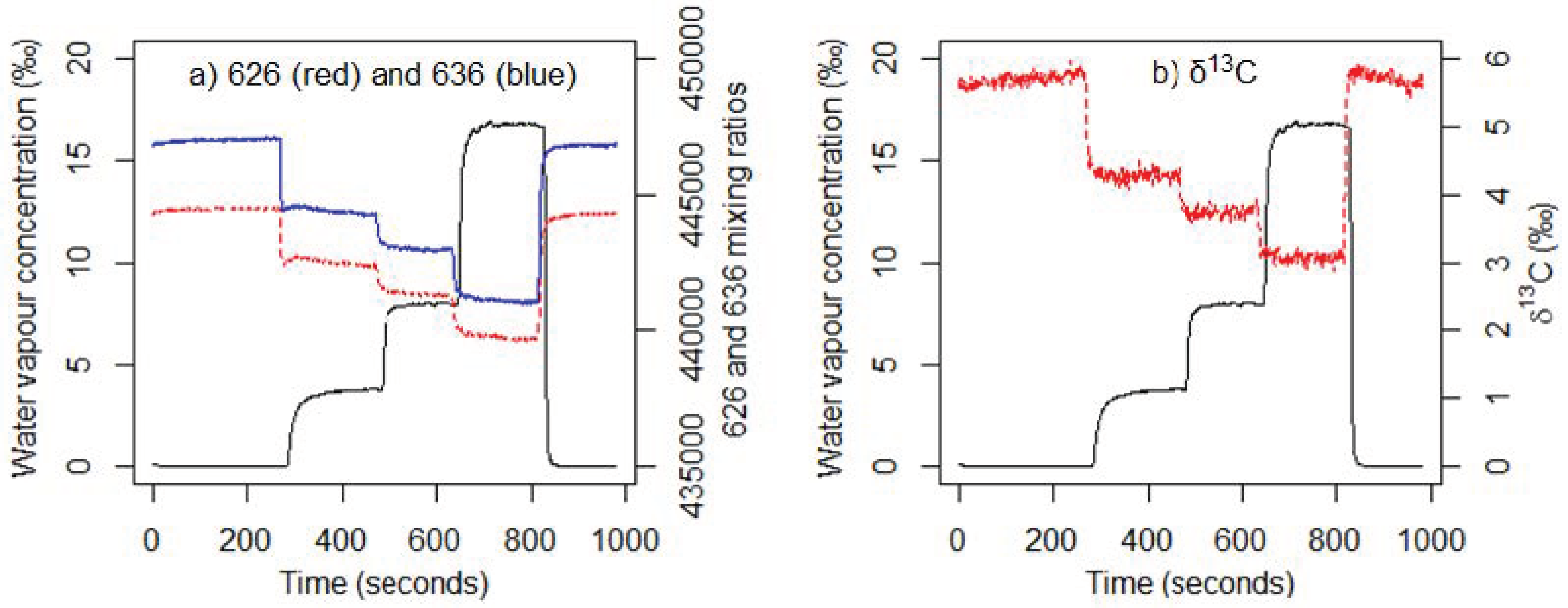
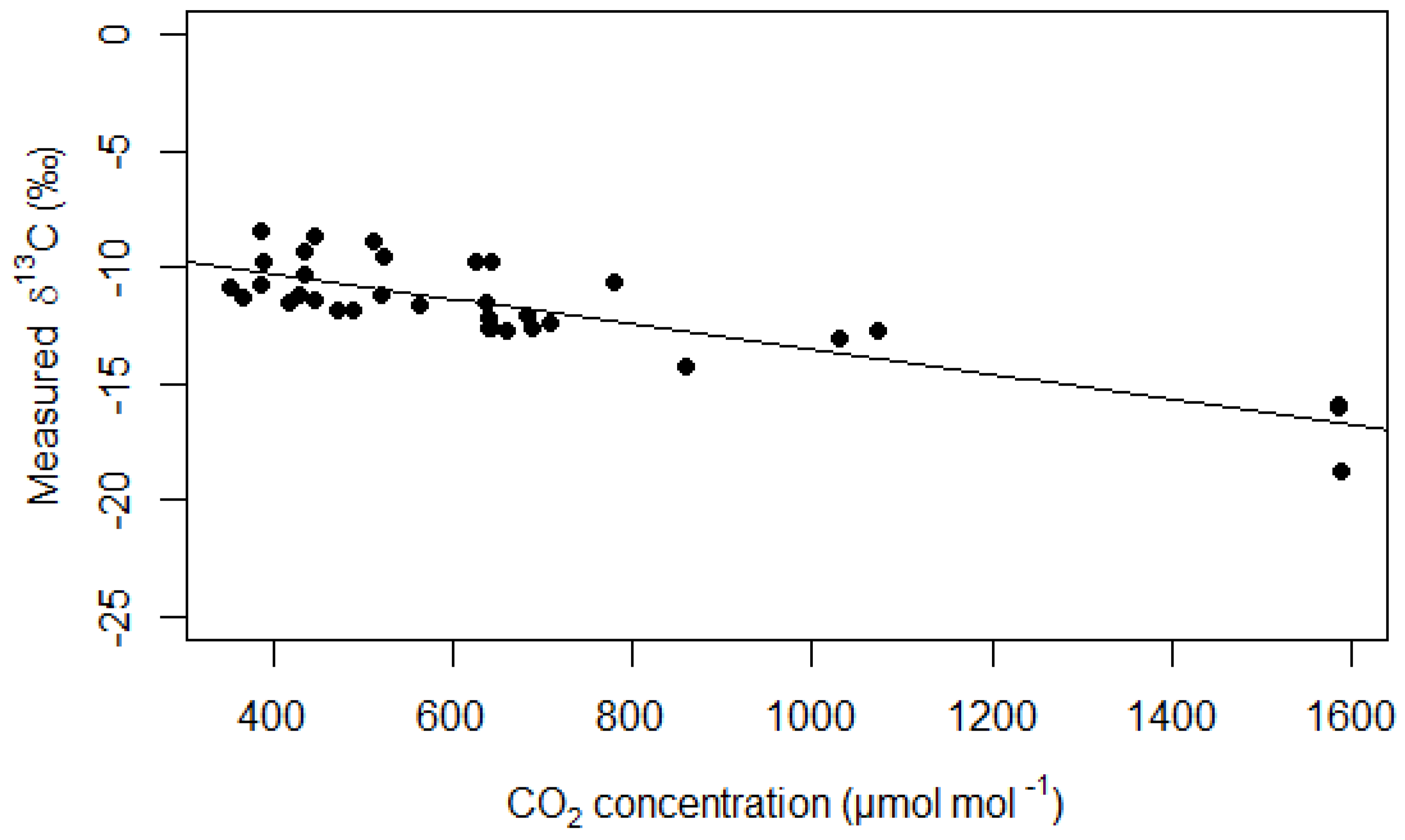
2.5. Test for Water Vapour and CO₂ Concentration Dependence

To allow for accurate and un-biased measurements of δ¹³C, the effect of sample water vapour and absolute CO₂ concentration on the measured δ¹³C was determined.

The mixing ratios of the isotopologues ¹⁶O¹²C¹⁶O and ¹⁶O¹³C¹⁶O measured by the QCL system are reported by the TDL Wintel software following the high-resolution transmission molecular absorption database (HITRAN) notation as 626 and 636, respectively, which are scaled by standard isotopic abundances in ppb [31]. We will use the HITRAN notation in this paper. The effect of water vapour on measured 626 and 636 was determined by varying the water vapour content in a gas from a gas cylinder with a known δ¹³C (−24.47‰, determined by IRMS). We constructed a system where part of the gas from the gas cylinder could pass through a 20 L blue cap bottle containing tap water (a water bubbler) and part of the gas could bypass the water bubbler, controlled by two restriction valves before the air was let to the laser inlet. By varying the amount of gas that passed through the water bubbler, different water vapour contents of the gas could be made ranging from 0 mmol mol⁻¹ (completely bypassing the water bubbler) to 20 mmol mol⁻¹ (all gas passing through the water bubbler). This spanned the concentration range of water vapour during the chamber measurements that typically was between 10 to 15 mmol mol⁻¹. The QCL system does not measure the water vapour content of the air. Thus, we connected a LI-7000 infrared gas analyser (LI-COR Environmental, Lincoln, NE, USA) to the outlet of the QCL system to measure water vapour concentration. The results were used to calculate the water vapour dilution effect and the vapour pressure line broadening (VPB) correction coefficient (α_v). From this we derived an equation to calculate the dry mixing ratios 626 and 636, which we then used to calculate the dry δ¹³C corrected for water vapour.

The dependence of sample CO₂ concentration on measured δ¹³C was determined by varying the CO₂ concentration while keeping the δ¹³C constant in a dry gas from a cylinder of known δ¹³C. The gas had a CO₂ concentration of 1590 ppm and a δ¹³C of −24.5‰ (determined by IRMS). Samples with different CO₂ concentrations were made by mixing the gas of known δ¹³C with CO₂ free synthetic air from a gas cylinder into a 20 L plastic bag. The CO₂ concentration and δ¹³C of the sample were then measured by placing the QCL system inlet tube in the plastic bag. Different mixes ranging from 350 ppm to 1590 ppm were made during a 3-h experiment. The relationship between measured δ¹³C and the CO₂ concentration of the sample was quantified by linear regression.

2.6. Data Analysis

All data analysis was performed in R version 3.2.0 [32]. From the raw QCL system data of 626 and 636, a corrected δ¹³C was calculated from the calibration with the gas of known δ¹³C and by including the experimentally determined impact of CO₂ concentration and water vapour of the sample on the measured mixing ratios of 626 and 636. Subsequently, the δ¹³C of the CO₂ for each chamber measurement was determined by the Keeling plot method.

For each chamber measurement, the data from the initial period of 120 s after chamber closure was discarded (the dead band) from further analysis. This relative long dead band was necessary to ensure adequate mixing of air between the QCL system and the LI-8100A/8150 system.

The mixing ratios of 626 and 636 were corrected based on the empirically determined effects of water vapour on the measured mixing ratios (see Section 3.1.). From this, the dry δ¹³C corrected for water vapour was calculated in accordance with TDL Wintel manual as

$${\delta }^{13}{C}_{dry}=\left(\frac{{\chi }_{636}^{\mathrm{dry}}}{{\chi }_{626}^{\mathrm{dry}}}-1\right)1000$$

(1)

where ${\chi }_{636}^{\mathrm{dry}}$ and ${\chi }_{626}^{\mathrm{dry}}$ are the dry mixing ratios of 636 and 626, respectively. In the second step, the δ¹³C was corrected for the effect of sample CO₂ concentration based on the empirical relationship observed between CO₂ concentration and measured δ¹³C. The δ¹³C was normalised to a CO₂ concentration of 400 ppm. Finally, the fully corrected δ¹³C was calculated by correcting for the difference in the measurement of calibration gas δ¹³C between the QCL system and the IRMS. During the measurement campaign, the calibration gas was measured every two hours and linear interpolation between two adjacent calibrations was used to get a specific δ¹³C calibration value at any given time between calibrations, that is, during chamber measurement. From the fully corrected δ¹³C values, the δ¹³C of the CO₂ flux was determined for each chamber measurement by applying the Keeling plot method [10]. This means that for each chamber measurement, the fully corrected δ¹³C was fitted against the reciprocal dry CO₂ concentration by linear regression and the δ¹³C of the CO₂ flux was determined as the intercept with the y-axis from the linear regression. The Keeling plot method was also used on δ¹³C data where no calibrations had been applied to the measured δ¹³C, where δ¹³C had been calibrated against the calibration gas and where only the CO₂ concentration dependence correction had been applied, respectively, to examine the individual effects of the corrections on the final δ¹³C determined by the Keeling plots. A CO₂ flux was calculated as well for each measurement on a time and soil, root or stem surface area basis by applying a linear regression to the increase in chamber CO₂ concentration during chamber closure time similarly to Reference [33].

δ¹³C values determined by the Keeling plots were removed from further analysis if the difference in the raw measured δ¹³C values between two adjacent calibrations was higher than 2.5‰. This was done to discard data from periods when internal drift in the QCL system was high. In addition, data were discarded from further analysis if the linear Keeling plot regression produced R² < 0.90. Flagging of data with an R² value lower than 0.9 of the linear Keeling plot regression, removed 662 (8.4%) of the measurements and flagging of data with a difference in the δ¹³C value higher than 2.5‰ between the calibrations made every two hours removed 593 (7.6%) of the data. This left 6588 chamber measurements for the two-month measurement campaign.

From the remaining δ¹³C values determined by the Keeling plots, the data was investigated to examine differences between plots and variation in δ¹³C on a seasonal and diel timescale. The mean δ¹³C for the entire two-month measurement period as well as the diel pattern of δ¹³C were calculated for each plot in the following way. First, the mean δ¹³C was calculated for each of the 12 times of the day. This provided the diel pattern δ¹³C across the day. Then, the mean daily δ¹³C for each plot was calculated from the 12 δ¹³C values.

3. Results

3.1. Water Vapour and CO₂ Concentration Dependence

The measured mixing ratios of 626 and 636 were lower in wet compared to dry air and water vapour affected the two species differently resulting in a negative relationship between measured δ¹³C and water vapour concentration (Figure 2). The results were used to parameterise the equation for the VPB correction coefficient for both species, which we could use to calculate the dry mixing ratios of a sample containing water vapour:

$${\chi }_{626}^{\mathrm{dry}}=(1+{\alpha }_{v626}\times {\chi }_{\mathrm{H}2\mathrm{O}})\times {\chi }_{626}$$

(2)

and

$${\chi }_{636}^{\mathrm{dry}}=(1+{\alpha }_{v636}\times {\chi }_{\mathrm{H}2\mathrm{O}})\times {\chi }_{636}$$

(3)

where ${\alpha }_{v626}$ and ${\alpha }_{v636}$ are the experimentally determined VPB correction coefficients of 0.006092 1000/mol H₂O and 0.007694 1000/mol H₂O for 626 and 636, respectively. ${\chi }_{\mathrm{H}2\mathrm{O}}$ is the measured content of water vapour in the sample in ‰ and ${\chi }_{626}$ and ${\chi }_{636}$ are the measured raw mixing ratios of 626 and 636 from the QCL system, respectively, in ppb following the HITRAN notation. The dilution effect accounts for 1 (mol H₂O)⁻¹ and the line broadening effect is thus 5.092 and 6.694 (mol H₂O)⁻¹ for ${\chi }_{626}$ and ${\chi }_{636}$, respectively. The extra effect from pressure line broadening would under the field conditions, where ${\chi }_{\mathrm{H}2\mathrm{O}}$ ranged between 10 and 15‰, account for 6.1 to 9.1% for ${\chi }_{626}$ and 7.7 to 11.5% for ${\chi }_{636}$.

The experiment to test the effect of sample CO₂ concentration on the measured δ¹³C values, that is, when the ${\chi }_{626}$ was changed and the δ¹³C was kept constant, showed a negative relationship between CO₂ concentration and measured δ¹³C (Figure 3). We used linear regression to describe this relationship (intercept: −8.1024, slope: −5.405 × 10⁻⁶, R² = 0.71), which corresponded to a decrease in δ¹³C of 0.54‰ per a 100 ppm increase in CO₂ concentration. We used the intercept and slope to derive the equation:

$${\delta }^{13}{C}_{dry, H2Ocorr}=\left(-5.405\times {10}^{-6}\times {\chi }_{626}^{\mathrm{dry}}-8.1014-{\delta }^{13}{C}_{ref}\right)+{\delta }^{13}$$

(4)

which was used to normalise the δ¹³C to a CO₂ concentration of 400 ppm, at which CO₂ concentration the true δ¹³C was known from the calibration gas. ${\delta }^{13}{C}_{ref}$ is the δ¹³C at a ${\chi }_{626}^{\mathrm{dry}}$ of 400000 ppb (400 ppm CO₂) and ${\delta }^{13}{C}_{dry}$ is the δ¹³C after being corrected for water vapour.

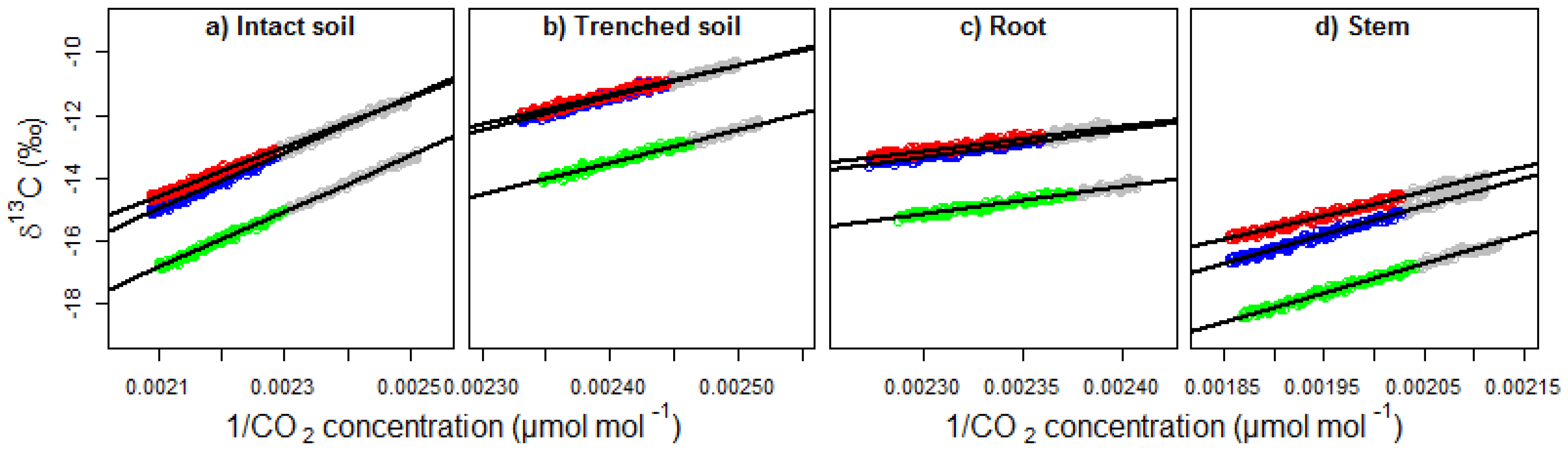
3.2. Effect of the δ¹³C Corrections on the Keeling Plots

The corrections for water vapour and CO₂ concentration dependence were both important but differed in their effect on the Keeling plots of the four different plot types measured with the automated chambers (Figure 4,

Table 1. The mean Keeling plot intercepts (the determined δ¹³C of the CO₂ flux) and slopes using the measured δ¹³C, the δ¹³C corrected for water vapour and the δ¹³C corrected for both water vapour and CO₂ concentration dependence, respectively. The means are shown for all measurements together and individually for intact soil, trenched soil, roots and stems, respectively. All δ¹³C values were calibrated against a standard calibration gas with known δ¹³C.

Plot Type	Keeling Plot Parameter	Using Measured δ13C	Using δ13C Corrected for Water Vapour	Using δ13C Corrected for Water and CO2
All	Intercept	−35.7 ± 2.9	−33.6 ± 2.8	−30.2 ± 2.9
	Slope	9577 ± 1304	9588 ± 1325	8164 ± 1329
Intact soil	Intercept	−35.3 ± 2.6	−33.1 ± 2.6	−29.8 ± 2.7
	Slope	9412 ± 1176	9370 ± 1172	7958 ± 1212
Trenched soil	Intercept	−35.1 ± 2.9	−32.8 ± 2.8	−29.7 ± 2.9
	Slope	9272 ± 1277	9251 ± 1265	7954 ± 1288
Roots	Intercept	−37.4 ± 3.0	−35.5 ± 3.0	−32.6 ± 2.9
	Slope	10246 ± 1415	10415 ± 1433	9214 ± 1380
Stems	Intercept	−36.2 ± 2.5	−34.3 ± 2.5	−30.2 ± 2.4
	Slope	9901 ± 1261	9959 ± 1279	8134 ± 1206

).

Both corrections increased the intercept with the y-axis of the Keeling plots and thus the determined δ¹³C estimate of the source of the CO₂ flux in all cases. The water vapour correction increased the mean δ¹³C for all measurements by 2.1‰ (from −35.7 ± 2.9‰ to −33.6 ± 2.8‰, Table 1), while the additional CO₂ concentration dependence correction had a higher effect by increasing the overall mean δ¹³C by 3.4‰ (to −30.2 ± 2.9‰). For the water vapour correction, only small differences were seen between the four plot types. In contrast, the CO₂ concentration dependence correction had the largest effect on the stem measurements followed by the intact soil, trenched soil and roots, yielding increases of the measured δ¹³C of 4.1, 3.3, 3.1 and 2.9‰, respectively. No change was seen in the slope of the Keeling plot from the water vapour correction (Table 1). This contrasted with the CO₂ concentration dependence correction, which on average decreased the slope by 14.9% (from 9588 ± 1325 to 8164 ± 1329). The biggest decrease was seen for the stem chambers, followed by the intact soil, trenched soil and root chambers, which decreased by 18.3, 15.1, 14.0 and 11.5%, respectively.

The δ¹³C of the standard calibration gases varied from −10.48 to −9.39‰ as measured by IRMS. The δ¹³C measured by the QCL system during the calibrations was, however, on average 17.85‰ lower than the δ¹³C of the standard gases, with a standard deviation of 1.19. Thus, in the final step of the calibration, on average 17.85‰ was added to the δ¹³C corrected for water vapour and CO₂ concentration dependence to give the fully calibrated absolute value of δ¹³C.

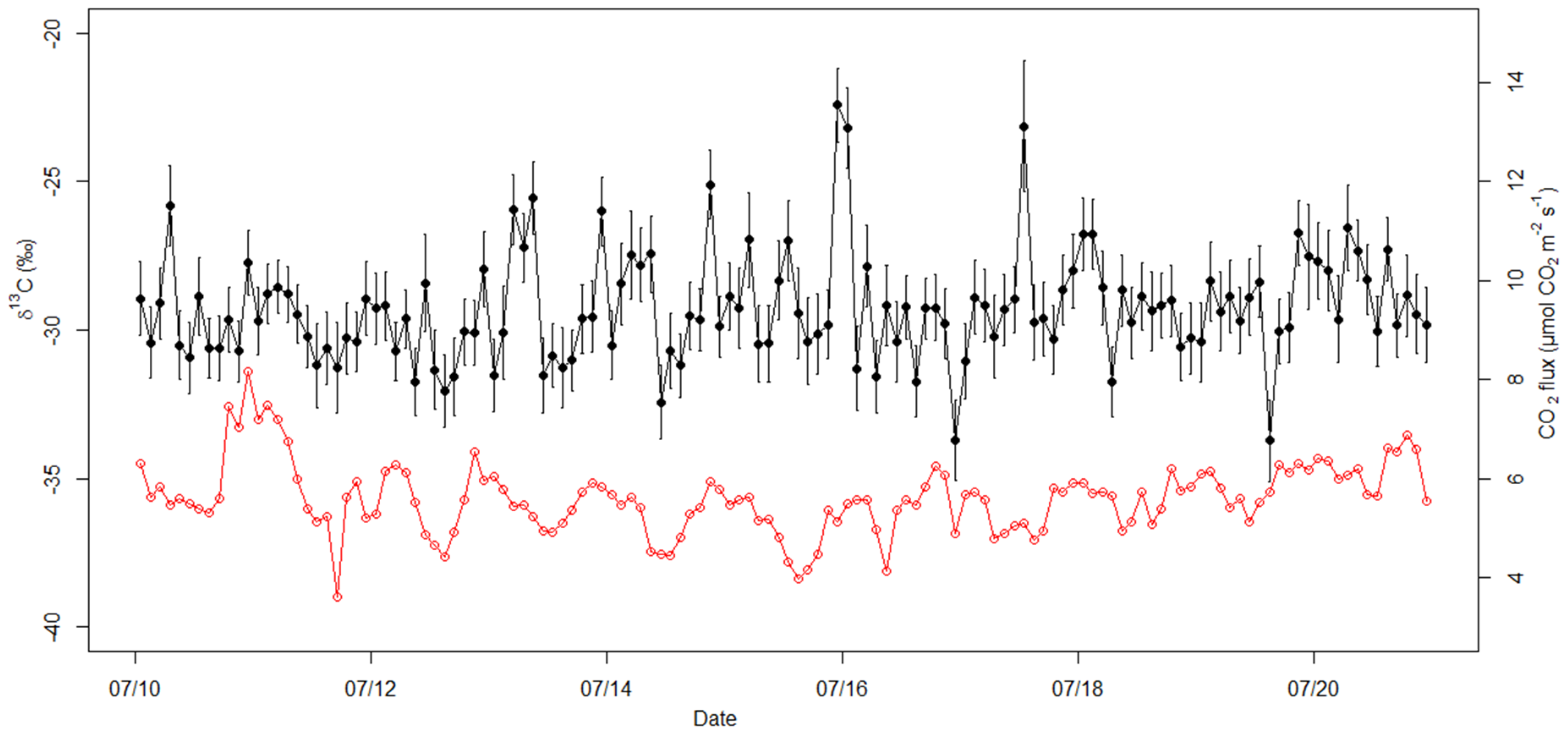
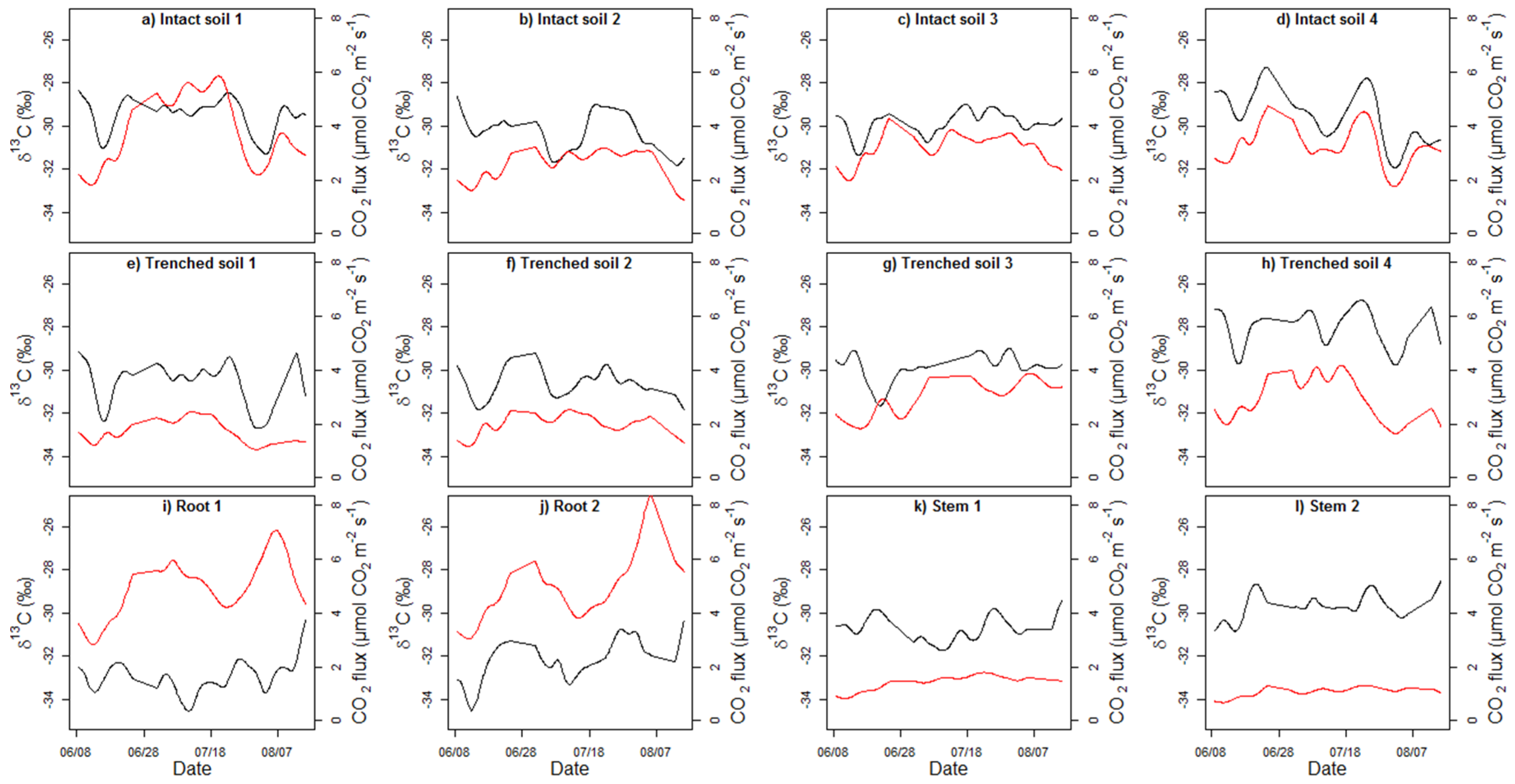
3.3. Automated Chamber Measurement Campaign

Both the CO₂ fluxes and the δ¹³C of the CO₂ fluxes showed considerable variation over time (Figure 5).

To compare the δ¹³C of the CO₂ flux from the four different plot types, we calculated the mean δ¹³C for each of the 12 plots (Figure 6). The mean δ¹³C for all plots was −30.3 ± 1.3‰. The mean δ¹³C for intact soil plots was −29.8 ± 0.32‰ with only small differences between the four plots. The δ¹³C for the trenched soil plots was similar to the intact soil plots with a mean δ¹³C of −29.8 ± 1.2‰. One of the trenched soil plots (Trenched soil 4), however, had a δ¹³C of −28.0 ± 0.32‰, higher than any of the δ¹³C for the intact soil plots, while the other three trenched soil plots had a mean δ¹³C of −30.4 ± 0.41‰, slightly lower than the intact soil plots. The two root plots had the lowest δ¹³C of all plots with δ¹³C values of −33.1 ± 0.88‰ and −32.0 ± 0.35‰ for Root 1 and Root 2, respectively, resulting in a mean δ¹³C of −32.6 ± 0.78‰. Finally, the two stem plots showed δ¹³C values of −30.7 ± 0.28‰ and −29.7 ± 0.43‰ for Stem 1 and Stem 2, respectively, resulting in a mean δ¹³C of −30.2 ± 0.74‰, which was similar to the mean δ¹³C of the trenched plots.

CO₂ flux measurements with the LI-8100A/8150 system had been performed since January 2016 [29]. This allowed for examining the effect of trenching on the CO₂ fluxes, by looking at the CO₂ fluxes from the intact and trenched plots in January, February and March, before the trenching on 6 April and during the laser campaign in June, July and August. For January, February and March, the trenched plot 1, 2, 3 and 4 accounted for 70.9, 83.9, 119.5 and 100.9%, respectively, of the mean CO₂ flux for the intact soil plots. However, during the QCL system measurement campaign they only accounted for 55.5, 62.4, 91.6 and 91.4%, respectively, corresponding to a decrease relatively to the intact soil plots of 21.7, 25.6, 23.4 and 9.4%, respectively.

The mean δ¹³C for each plot was based on two months of measurements. Thus, to examine the consistency of the mean throughout the measurement campaign and to see if any day to day variability and seasonality was present (Figure 7), we looked at δ¹³C as well as the CO₂ fluxes for each plot throughout the entire period. The intact soil, trenched soil and stem plots generally showed an increase in CO₂ fluxes during the first quarter of the measurement period, followed by a period of high fluxes and finally lower fluxes again by the end of the measurement period. This temporal pattern followed the soil temperature measured at 5 cm depth (Figure 8). The two root plots differed; however, by showing two peak periods of CO₂ fluxes during the measurement period (Figure 7i,j). In contrast to the CO₂ fluxes, δ¹³C showed no clear pattern across the two months. The δ¹³C for each plot did, however, show some day to day variability, with δ¹³C values typically ranging within 2–3‰ depending on plot.

For a few plots (e.g., intact soil 4, Figure 7d), an apparent relationship between the CO₂ flux and δ¹³C was seen, with higher CO₂ fluxes resulting in higher δ¹³C values. To examine this further, we performed a linear regression between CO₂ flux and δ¹³C for each plot. We also performed a linear regression between soil temperature at 5 cm depth and δ¹³C. A significant positive linear relationship was found between CO₂ flux and δ¹³C for all plots, except Trenched soil 3 and Root 1. R² values were, however, generally low (

Table 2. Results of the linear regressions between the CO₂ fluxes and δ¹³C of the CO₂ fluxes and the linear regressions between the soil temperature at 5 cm depth and δ¹³C of the CO₂ fluxes for each plot. For each regression, the adjusted R², slope and p-value are shown. A p-value in bold indicate a significant p-value.

Plot	CO2 Flux and δ13C			Soil Temperature and δ13C
	Adjusted R2	Slope ± SE	p-Value	Adjusted R2	Slope ± SE	p-Value
Intact soil 1	0.051	0.41 ± 0.071	<0.001	−0.00071	0.059 ± 0.077	0.45
Intact soil 2	0.04	0.81 ± 0.16	<0.001	0.0071	0.18 ± 0.080	<0.05
Intact soil 3	0.043	0.66 ± 0.13	<0.001	0.0071	0.18 ± 0.075	<0.05
Intact soil 4	0.15	0.93 ± 0.085	<0.001	0.0003	−0.081 ± 0.074	0.276
Trenched soil 1	0.054	1.4 ± 0.26	<0.001	−0.002	−0.010 ± 0.098	0.92
Trenched soil 2	0.033	0.98 ± 0.27	<0.001	0.01	0.22 ± 0.089	<0.05
Trenched soil 3	−0.0019	0.11 ± 0.19	0.56	−0.0012	0.096 ± 0.13	0.45
Trenched soil 4	0.048	0.44 ± 0.080	<0.001	−0.0013	0.038 ± 0.071	0.59
Root 1	0.04	0.42 ± 0.090	<0.001	−0.0018	0.035 ± 0.11	0.74
Root 2	0.052	0.50 ± 0.10	<0.001	0.023	0.37 ± 0.11	<0.01
Stem 1	−0.0016	0.018 ± 0.27	0.95	−0.0014	0.025 ± 0.062	0.68
Stem 2	0.0056	1.0 ± 0.49	<0.05	0.0072	0.16 ± 0.071	<0.05

). For soil temperature and δ¹³C, a significant positive relationship was only found for five plots. As for CO₂ flux and δ¹³C, R² values were low.

We calculated the mean diel pattern of δ¹³C and CO₂ fluxes for the entire measurement period for each plot (Figure 9). For the intact soils (Figure 9a–d) and the trenched soils (Figure 9e–h), the CO₂ fluxes were generally higher during the night-time than during daytime. Root 1 and the stem plots, however, showed the highest fluxes during daytime, while Root 2 showed the highest fluxes between 04:00 and 08:00 CET. The diel pattern of δ¹³C showed a larger variation within groups than the CO₂ fluxes. δ¹³C for a plot was generally within a 1–3‰. For some plots no apparent diel pattern was observed (Intact soil 3, Trenched soil 1, Trenched soil 3, Root 2, Stem 1 and Stem 2). The remaining plots, however, showed varying degrees of diel fluctuation. Intact soil 1, 2 and 4 showed highest δ¹³C values during night-time and lowest δ¹³C values during daytime. The difference between the daytime average (09:00 to 15:00 CET) and night-time average (21:00 to 03:00 CET) was 0.65, 0.93 and 0.92‰ for Intact soil 1, 2 and 4, respectively, with Intact soil 4 showing the largest difference of 1.98‰ between two hours of the day (−28.4‰ at 04:00 CET and −30.4 at 08:00 CET). Trenched soil 2 showed a moderate diel pattern similar to the intact soil plots, with the lowest δ¹³C of −31.4‰ at 10:00 CET and the highest δ¹³C of −30.0‰ at 00:00 CET. The diel pattern of δ¹³C for Trenched soil 4 differed by showing the highest δ¹³C values late in the afternoon and the lowest δ¹³C values early in the morning, with the highest and lowest δ¹³C values of −27.5 and −28.6‰ at 16:00 and 06:00 CET, respectively. Root 1 showed the largest diel pattern of any plot with the lowest δ¹³C of −34.7‰ seen at 04:00 CET. From 04:00 CET, δ¹³C increased until 10:00 CET (a δ¹³C of −32.1‰) and remained high until 18:00 CET (a δ¹³C of −32.0‰).

4. Discussion

4.1. Effect of the δ¹³C Corrections

The corrections for water vapour and CO₂ concentration dependence both lowered the δ¹³C, which consequently lowered the estimated δ¹³C of the CO₂ fluxes determined by the Keeling plots during the automated closed-chamber campaign (Figure 4, Table 1). Although the CO₂ concentration dependence correction only slightly changed the δ¹³C, it had the largest impact on the δ¹³C determined from the Keeling plots, because it changed the slope of the plots. The change in CO₂ concentration and δ¹³C during a measurement is inherent to the closed-chamber method for determination of the δ¹³C of the source by the Keeling plot method. Our results highlight the importance of the CO₂ concentration dependence correction, which is likely more important for closed-chamber measurements than, for example, for eddy covariance measurements, where the δ¹³C is measured at an atmospheric CO₂ concentration with small absolute fluctuation during a flux sample. Direct comparison of our results with previous studies is not possible because no one else has previously combined an Aerodyne CO₂ isotope QCL system with the LI8100A/LI8150 system for automated closed-chamber measurements. However, the issues of dependence of water vapour and especially CO₂ concentration on measured δ¹³C have been addressed in a few studies using laser spectroscopy methods, including quantum cascade lasers [19,23,24,25,34]. In a study where δ¹³C was measured with a quantum cascade laser spectrometer, [21] performed 90 closed-chamber measurements and determined the CO₂ concentration dependency but did not report the effect of this calibration on the raw δ¹³C values or the effect on the δ¹³C determined by the Keeling plots. [18] used an Aerodyne isotope quantum cascade laser spectrometer for eddy covariance measurements and also characterised the instrument’s CO₂ concentration dependence but likewise did not report the results. [35] compared two cavity ring-down spectroscopy analysers and found an increase in δ¹³C per 100 ppm of 0.46 and 0.09‰, respectively, for the two analysers. This is in contrast to our observation of a decrease in δ¹³C per 100 ppm of 0.54‰. [36], however, found no concentration dependency of δ¹³C in the CO₂ concentration range of 303–437 ppm. The same lack of CO₂ concentration dependency was found for the quantum cascade laser spectrometer developed by [13]. Taken together, it is clear that large differences in the CO₂ concentration dependence between different laser spectroscopy instruments exist. However, the reason for the concentration dependence remains unresolved [37]. Based on this study and previous studies using laser spectrometers for δ¹³C measurements, we recommend quantifying the CO₂ concentration dependence for each instrument, for example, by using the approach described in this study.

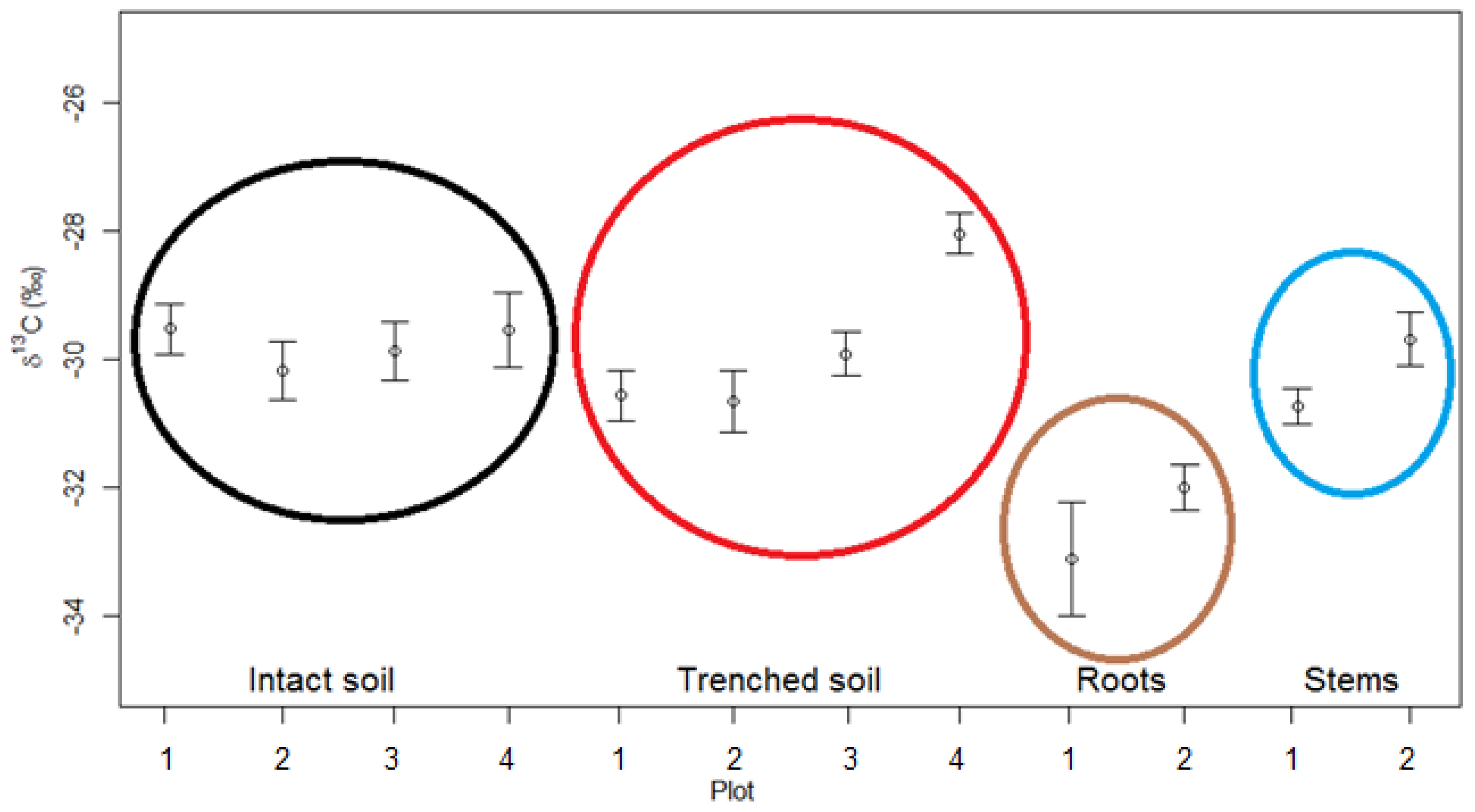
4.2. Overall δ¹³C Values of the CO₂ Fluxes From Intact Soils, Trenched Soils, Roots and Stems

The δ¹³C signatures from heterotrophic and autotrophic R_soil have previously been measured at the DK-Sor site using manually taken air samples followed by isotopic analysis by IRMS [38] and the results of the partitioning of soil respiration into heterotrophic and autotrophic components were independently confirmed by [39]. It has been found that δ¹³C from heterotrophic respiration of soil organic matter is enriched compared to δ¹³C from autotrophic respiration, with the resulting δ¹³C of R_soil from intact soil falling in between, because it is a mix of heterotrophic and autotrophic respiration [38,40]. This has been used to partition R_soil into heterotrophic and autotrophic respiration by applying a linear mixing model, thus providing measurements of process-based fluxes, which can be used to improved process-based CO₂ flux models [38]. Ideally, the intact soil plots contain both roots and soil organic matter, whereas the trenched plots do not contain any live roots. The lower root δ¹³C compared to both the intact and trenched soil, fits well the generally depleted δ¹³C observed for roots [40]. However, we found a similar mean δ¹³C for the intact and trenched plots, which disagrees with earlier studies that found higher δ¹³C for heterotrophic R_soil [41]. The trenched soil plot 4 had a δ¹³C of −28.0 ± 0.32‰ and was thus the only plot with a δ¹³C higher than the three other trenched plots and the intact soil plots. This is in line with the higher δ¹³C observed for soil organic matter. It remains unexplained why we did not see a difference in δ¹³C between the three other trenched plots and the intact soil plots. One possibility is an unsuccessful trenching. Examining the CO₂ fluxes for the four trenched plots before and after the trenching, suggested a decrease in R_soil ranging from 9.4% to 25.6% for the four trenched plots. This is a relative low decrease based on previous studies of the autotrophic contribution to R_soil [42,43,44], which could indicate an unsuccessful trenching. However, it is possible that the high R_soil for the trenched plot was due to respiration of root litter from roots severed by the trenching, which was performed only two months prior to beginning of the measurements [45,46,47]. In a previous study at the site, the δ¹³C of the solid material of fine roots, that made up more than a third of the root biomass, was found to be depleted in δ¹³C compared to the soil organic matter [38]. Thus, we expect that the decomposition of the fine roots following a trenching would result in an input to R_soil of CO₂ depleted in δ¹³C compared to the δ¹³C of CO₂ from the decomposition of the remaining soil organic matter.

The mean δ¹³C of the two stem plots was −30.2 ± 0.74‰, a value close to the δ¹³C of the soil plots but enriched compared to the δ¹³C of the root plots. Stem CO₂ flux is typically composed of respiration from the stem. However, it has been found that passive diffusion of CO₂ out of the stem from water in the xylem that is being transported from the roots to the shoots, can contribute to the stem CO₂ flux as well [48]. The CO₂ concentration in the soil pores is high, typically several thousand ppm, which leads to CO₂ being dissolved in the soil water [49,50,51]. This water is taken up by the plant, why the xylem can contain dissolved CO₂. We expect that the δ¹³C of the CO₂ dissolved in the soil water reflects the δ¹³C of R_soil. Thus, if a large part of the stem CO₂ flux is derived from this dissolved CO₂, then the δ¹³C of the stem CO₂ flux would reflect this. We measured a δ¹³C for the stem CO₂ flux close to the δ¹³C of R_soil, which indicates that passive diffusion out of the stem of CO₂ from R_soil could play a major role in the stem CO₂ flux at our site.

The mean δ¹³C for all plots was −30.3 ± 1.3‰. Values of δ¹³C from respired CO₂ from forest ecosystems have been found to lie in the range from −24 to −30‰ [1]. A previous study at the site gave mean values of −23.6 to 21.2‰ for different layers of soil organic matter and −22.2‰ for roots [38]. Thus, the δ¹³C values found in this study are in the lower range of reported literature values and consistently lower than δ¹³C values previously determined at the site. The δ¹³C values found by [38] were obtained by manual measurements with gas samples being analysed by IRMS. As discussed in Section 4.1, we found the measured δ¹³C to be influenced by water vapour and CO₂ concentration and consequently we corrected the measured δ¹³C. However, failing to accurately correct for these effects will lead to wrong δ¹³C values determined from the Keeling plots. It is possible that the different δ¹³C values in the two studies were due to instrumental differences, for example, because of the corrections for water vapour and CO₂ concentration of QCL system compared to the IRMS where the gas was purified prior to analysis. In some studies, the Keeling plot method has been found to be biased by diffusive fractionation, which can cause nonlinear Keeling plots, thus violating the basic principle of this method [52]. This can lead to a deviation in the determined δ¹³C value of the Keeling plot of up to 4‰ [52]. The Keeling plots in this study, however, were highly linear with generally high R² values and we only used measurements with a R² value higher than 0.9 in the analysis (Figure 4). Thus, it is unlikely that diffusive fractionation has had a major influence the determined δ¹³C values in this study. In addition, there is uncertainty attached to the determined δ¹³C value of the Keeling plot even without diffusive fractionation. In an analysis of 146 Keeling plots from 33 different field sites, [53] found a mean standard error for the Keeling plots of 1.2‰.

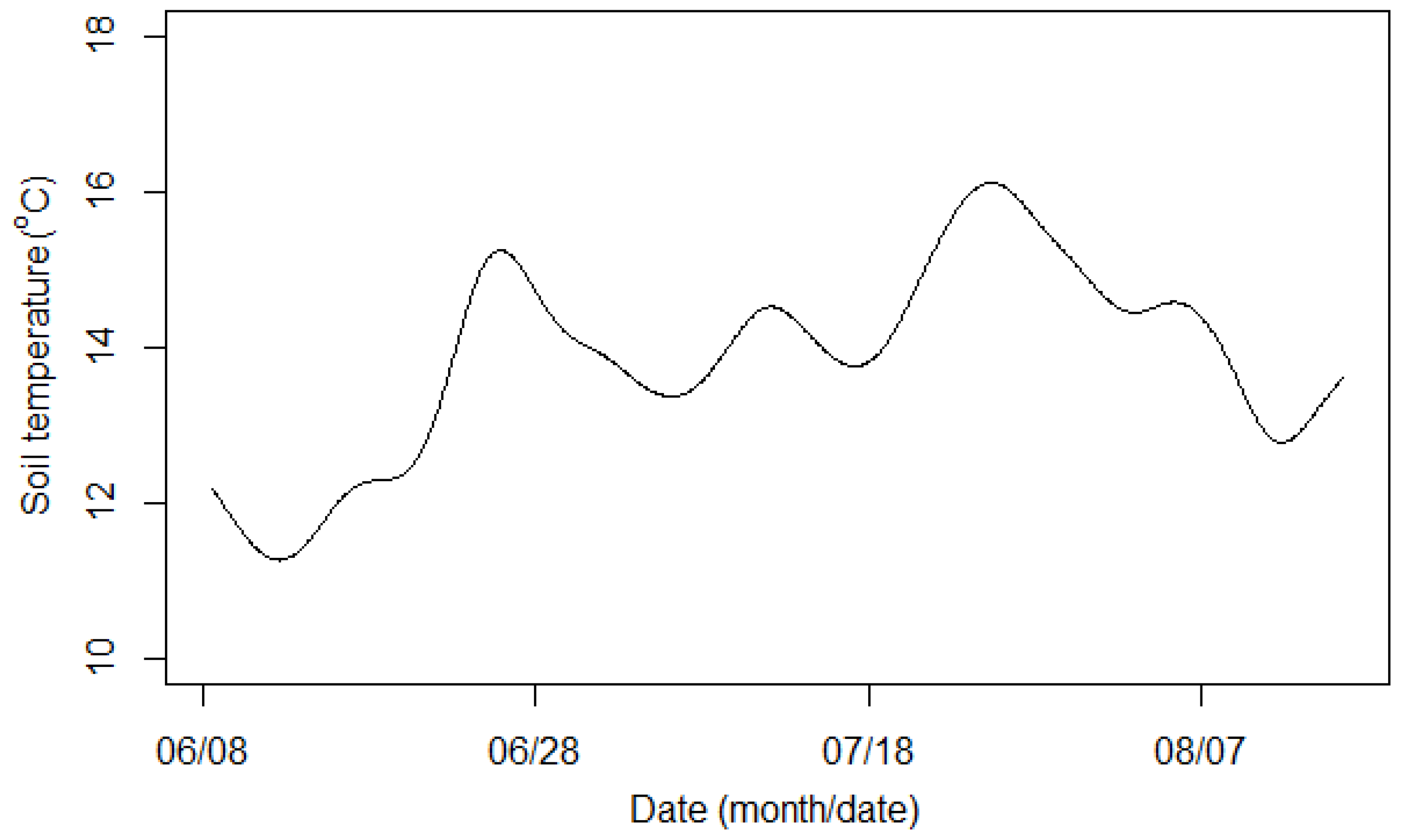
4.3. Seasonality of δ¹³C and Correlation with Flux and Temperature

No major change in δ¹³C for the different plots was observed during the two-month measurement period. The δ¹³C for each plot did, however, show some day to day variability, with δ¹³C values typically ranging within 2–3‰, depending on plot (Figure 7). Any change in δ¹³C of the respired CO₂ from a plot can be due to either a change in δ¹³C from a source, for example, a change in δ¹³C from bacterial or root respiration or a change in the individual respiratory contribution of each source that make up the δ¹³C of a plot [54]. Heterotrophic and autotrophic respiration have been found to respond differently to factors such as temperature and photosynthesis, with root respiration being more temperature sensitive than respiration of soil organic matter [55,56]. To examine the cause for the observed day to day variability in δ¹³C across the two months, we tested the relationship between δ¹³C and the CO₂ flux and the soil temperature, respectively (Table 2). A significant positive relationship was found between δ¹³C and soil temperature for two out of four intact soil plots. The two significant relationships are in contrast to what could be expected, if the roots were to respond more to temperature than the heterotrophic organisms. We found the lowest δ¹³C of respiration from roots. Thus, if a higher temperature would result in higher root respiration compared to heterotrophic respiration, then we would expect the δ¹³C of total R_soil in the intact soil plots to decrease. The linear regressions between δ¹³C and the CO₂ flux were significant for all plots except two. The day to day variation of R_soil has often been found to be caused by changes in temperature and photosynthetic input. The higher δ¹³C found in relation to CO₂ flux in the intact soils, does not support that root respiration represents a larger part of the total R_soil at higher fluxes. However, other reasons for the significant relationship between δ¹³C and the CO₂ flux are possible such as changing pathways or shifts in substrate [57,58].

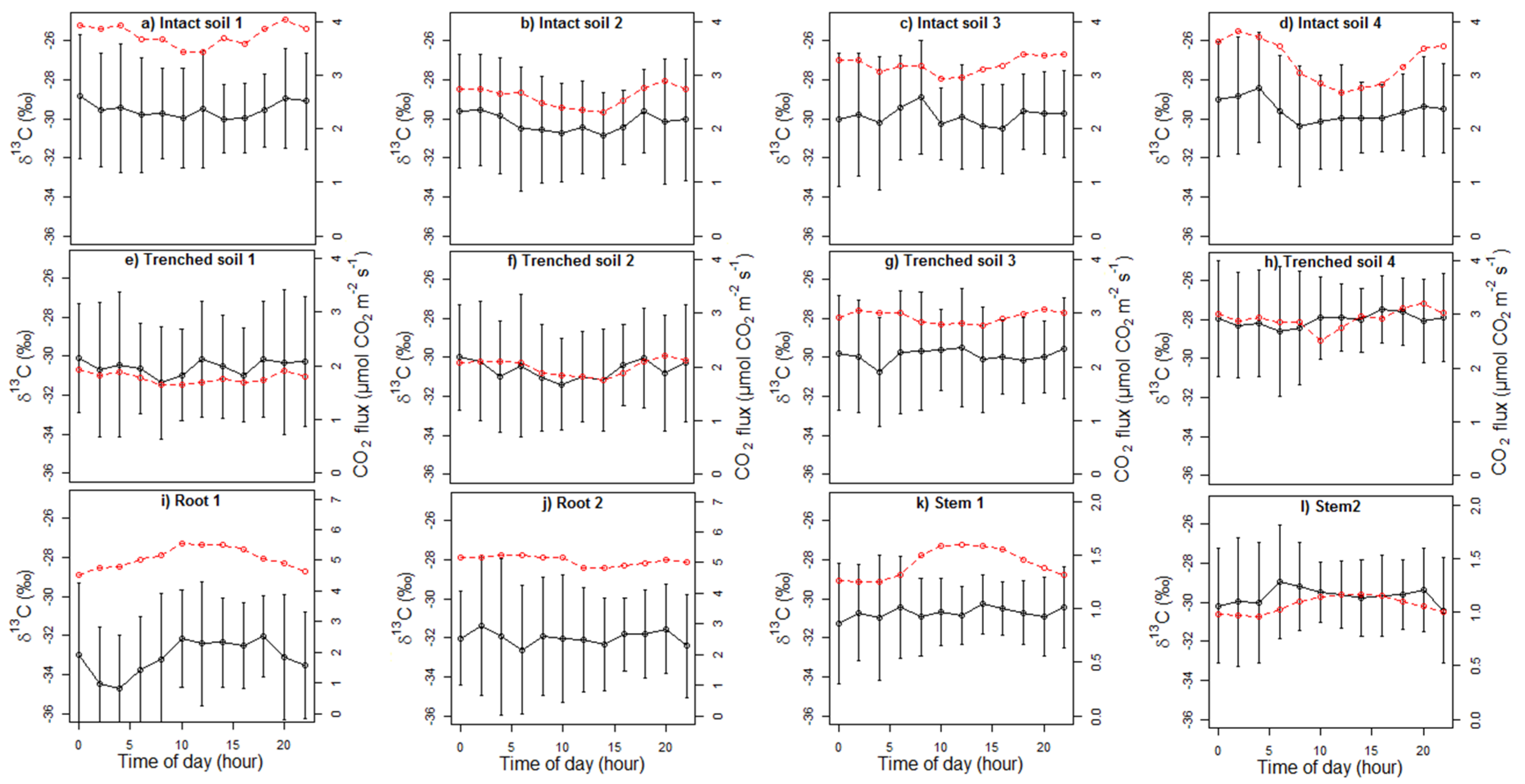
4.4. Diel Patterns of δ¹³C

The diel patterns of the δ¹³C of the CO₂ fluxes showed a high degree of variability with a clear diel pattern for some plots, whereas other plots showed no distinct pattern (Figure 9). However, when considering the variability, no significant diel patterns could be identified. Most of the processes that govern the day to day and seasonal variation in δ¹³C may also operate on shorter timescales, thereby potentially causing a diel pattern of δ¹³C. For stems, a distinct diel pattern has been found with highest δ¹³C of the CO₂ fluxes during daytime [59], whereas the two stems in our study showed no distinct difference between daytime and night-time δ¹³C (Figure 9). In contrast, the stem CO₂ fluxes showed a clear diel pattern with highest fluxes during daytime. This may be related to higher temperature, as well as to higher diffusion of CO₂ out of the stems due to higher upward xylem transport of soil water enriched with CO₂ originally produced in the soil [60].

The contribution of root respiration to soil respiration can vary on a diel timescale due to changes in photosynthesis and substrate supply, thereby changing the diel pattern of δ¹³C of the CO₂ flux from intact soil. Intact soil 1, 2 and 4 indeed showed a diel pattern with highest δ¹³C values during night-time and lowest δ¹³C values during daytime. This followed the CO₂ fluxes and the general relationship found by linear regression between δ¹³C and CO₂ flux. The low daytime δ¹³C indicates that root respiration contributes relatively more to total R_soil at daytime than during night-time. Normally the higher root respiration on a diel timescale would result in higher total R_soil. We, however, observed the opposite. It is possible that the CO₂ flux measurements during night-time observed in our study are overestimated due to occasionally insufficient mixing of air above the soil surface during low atmospheric turbulence conditions leading to apparently high flux estimates [33]. This potential bias may therefore complicate the interpretation of the measured diel patterns.

5. Conclusions

We successfully combined an Aerodyne quantum cascade laser spectrometer for CO₂ isotopes with an LI-8100A/8150 automated closed-chamber system to yield real-time δ¹³C of CO₂ fluxes during a two-month field campaign in a Danish beech forest. We generally found lower δ¹³C values compared to a previous study at the site and small differences in δ¹³C between different ecosystems compartments, that is, intact soil, trenched soil, tree stems and coarse tree roots. Furthermore, by thoroughly testing the instruments, we found that the δ¹³C measured by the laser spectrometer was influenced by the water vapour and CO₂ concentration of the sample air and we developed a method to correct for these effects to yield accurate measurements of δ¹³C.

In conclusion, the study showed the potential of using a quantum cascade laser spectrometer to measure δ¹³C of CO₂ during automated closed-chamber measurements, thereby allowing for high-temporal measurements of isotopic ecosystem CO₂ fluxes. It also highlighted the importance of proper correction for water vapour and CO₂ concentration of the sample air to get accurate measurements of δ¹³C.

References

1. Bowling, D.R.; Pataki, D.E.; Randerson, J.T. Carbon Isotopes in Terrestrial Ecosystem Pools and CO2 Fluxes. New Phytol. 2008, 178, 24–40. [Google Scholar] [CrossRef] [PubMed]
2. Farquhar, G.D.; Ehleringer, J.R.; Hubick, K.T. Carbon isotope discrimination and photosynthesis. Annu. Rev. Plant Physiol. Plant Mol. Biol. 1989, 40, 503–537. [Google Scholar] [CrossRef]
3. Park, R.; Epstein, S. Carbon isotope fractionation during photosynthesis. Geochim. Cosmochim. Acta. 1960, 21, 110–126. [Google Scholar] [CrossRef]
4. Janssens, I.A.; Lankreijer, H.; Matteucci, G.; Kowalski, A.S.; Buchmann, N.; Epron, D.; Pilegaard, K.; Kutsch, W.; Longdoz, B.; Grünwald, T.; et al. Productivity overshadows temperature in determining soil and ecosystem respiration across European forests. Glob. Chang. Biol. 2000, 7, 269–278. [Google Scholar] [CrossRef]
5. Rochette, P.; Hutchinson, G.L. Measurement of Soil Respiration in situ: Chamber Techniques. In Micrometeorology in Agricultural Systems; Agronomy Monograph 47; Hatfield, J.L., Baker, J.M., Eds.; American Society of Agronomy, Crop Science Society of America and Soil Science Society of America: Madison, WI, USA, 2005; pp. 247–286. [Google Scholar]
6. Edwards, N.T.; Riggs, J.S. Automated monitoring of soil respiration: A moving chamber design. Soil Sci. Soc. Am. J. 2003, 67, 1266–1271. [Google Scholar] [CrossRef]
7. Koskinen, M.; Minkkinen, K.; Ojanen, P.; Kämäräinen, M.; Laurila, T.; Lohila, A. Measurements of CO2 exchange with an automated chamber system throughout the year: Challenges in measuring night-time respiration on porous peat soil. Biogeosciences 2014, 11, 347–363. [Google Scholar] [CrossRef]
8. Liang, N.; Inoue, G.; Fujinuma, Y. A multichannel automated chamber system for continuous measurement of forest soil CO2 efflux. Tree Physiol. 2003, 23, 825–832. [Google Scholar] [CrossRef] [PubMed]
9. McGinn, S.; Akinremi, O.; McLean, H.; Ellert, B. An automated chamber system for measuring soil respiration. Can. J. Soil Sci. 1998, 78, 573–579. [Google Scholar] [CrossRef] [Green Version]
10. Keeling, C.D. The concentration and isotopic abundances of atmospheric carbon dioxide in rural areas. Geochim. Cosmochim. Acta 1958, 13, 322–334. [Google Scholar] [CrossRef]
11. Zeeman, M.J.; Werner, R.A.; Eugster, W.; Siegwolf, R.T.W.; Wehrle, G.; Mohn, J.; Buchmann, N. Optimization of automated gas sample collection and isotope ratio mass spectrometric analysis of δ13C of CO2 in air. Rapid Commun. Mass Spectrom. 2008, 22, 3883–3892. [Google Scholar] [CrossRef]
12. Bowling, D.R.; Sargent, S.D.; Tanner, B.D.; Ehleringer, J.R. Tunable diode laser absorption spectroscopy for stable isotope studies of ecosystem–atmosphere CO2 exchange. Agric. For. Meteorol. 2003, 118, 1–19. [Google Scholar] [CrossRef]
13. Guimbaud, C.; Noel, C.; Chartier, M.; Catoire, V.; Blessing, M.; Gourry, J.C.; Robert, C. A quantum cascade laser infrared spectrometer for CO2 stable isotope analysis: Field implementation at a hydrocarbon contaminated site under bio-remediation. J. Environ. Sci. 2016, 40, 60–74. [Google Scholar] [CrossRef] [PubMed]
14. Nelson, D.D.; McManus, J.B.; Herndon, S.C.; Zahniser, M.S.; Tuzson, B.; Emmenegger, L. New method for isotopic ratio measurements of atmospheric carbon dioxide using a 4.3 μm pulsed quantum cascade laser. Appl. Phys. B 2008, 90, 301–309. [Google Scholar] [CrossRef] [Green Version]
15. Tuzson, B.; Zeeman, M.J.; Zahniser, M.S.; Emmenegger, L. Quantum cascade laser based spectrometer for in situ stable carbon dioxide isotope measurements. Infrared Phys. Technol. 2008, 51, 198–206. [Google Scholar] [CrossRef]
16. Wahl, E.H.; Fidric, B.; Rella, C.W.; Koulikov, S.; Tan, S.; Kachanov, A.A.; Richman, B.A.; Crosson, E.R.; Paldus, B.A.; Kalaskar, S.; et al. Applications of cavity ring-down spectroscopy to high precision isotope ratio measurement of 13C/12C in carbon dioxide. Isotopes Environ. Health Stud. 2006, 42, 20–35. [Google Scholar] [CrossRef] [PubMed]
17. McManus, J.B.; Nelson, D.D.; Shorter, J.H.; Jimenez, R.; Herndon, S.; Saleska, S.; Zahniser, M. A high precision pulsed quantum cascade laser spectrometer for measurements of stable isotopes of carbon dioxide. J. Mod. Opt. 2005, 52, 2309–2321. [Google Scholar] [CrossRef]
18. Sturm, P.; Eugster, W.; Knohl, A. Eddy covariance measurements of CO2 isotopologues with a quantum cascade laser absorption spectrometer. Agric. For. Meteorol. 2012, 152, 73–82. [Google Scholar] [CrossRef]
19. Wehr, R.; Munger, J.W.; Nelson, D.D.; Mcmanus, J.B.; Zahniser, M.S.; Wofsy, S.C.; Saleska, S.R. Long-term eddy covariance measurements of the isotopic composition of the ecosystem–atmosphere exchange of CO2 in a temperate forest. Agric. For. Meteorol. 2013, 181, 69–84. [Google Scholar] [CrossRef]
20. Gentsch, L.; Sturm, P.; Hammerle, A.; Siegwolf, R.; Wingate, L.; Ogée, J.; Baur, T.; Plüss, P.; Barthel, M.; Buchmann, N.; et al. Carbon isotope discrimination during branch photosynthesis of Fagus sylvatica: Field measurements using laser spectrometry. J. Exp. Bot. 2014, 65, 1481–1496. [Google Scholar] [CrossRef]
21. Kammer, A.; Tuzson, B.; Emmenegger, L.; Knohl, A.; Mohn, J.; Hagedorn, F. Application of a quantum cascade laser-based spectrometer in a closed chamber system for real-time δ13C and δ18O measurements of soil-respired CO2. Agric. For. Meteorol. 2011, 151, 39–48. [Google Scholar] [CrossRef]
22. Guillon, S.; Pili, E.; Agrinier, P. Using a laser-based CO2 carbon isotope analyser to investigate gas transfer in geological media. Appl. Phys. B 2012, 107, 449–457. [Google Scholar] [CrossRef]
23. Pitt, J.R.; Le Breton, M.; Allen, G.; Percival, C.J.; Gallagher, M.W.; Bauguitte, S.J.-B.; O’Shea, S.J.; Muller, J.B.A.; Zahniser, M.S.; Pyle, J.; et al. The development and evaluation of airborne in situ N2O and CH4 sampling using a quantum cascade laser absorption spectrometer (QCLAS). Atmos. Meas. Tech. 2016, 9, 63–77. [Google Scholar] [CrossRef]
24. Wen, X.F.; Meng, Y.; Zhang, X.Y.; Sun, X.M.; Lee, X. Evaluating calibration strategies for isotope ratio infrared spectroscopy for atmospheric 13CO2/12CO2 measurement. Atmos. Meas. Tech. 2013, 6, 1491–1501. [Google Scholar] [CrossRef]
25. Griffith, D.W.T. Calibration of isotopologue-specific optical trace gas analysers: A practical guide. Atmos. Meas. Tech. 2018, 11, 6189–6201. [Google Scholar] [CrossRef]
26. Sturm, P.; Tuzson, B.; Henne, S.; Emmenegger, L. Tracking isotopic signatures of CO2 at the high altitude site Jungfraujoch with laser spectroscopy: Analytical improvements and representative results. Atmos. Meas. Tech. 2013, 6, 1659–1671. [Google Scholar] [CrossRef]
27. Pilegaard, K.; Hummelshøj, P.; Jensen, N.O.; Chen, Z. Two years of continuous CO2 eddy-flux measurements over a Danish beech forest. Agric. For. Meteorol. 2001, 107, 29–41. [Google Scholar] [CrossRef]
28. Pilegaard, K.; Ibrom, A.; Courtney, M.S.; Hummelshøj, P.; Jensen, N.O. Increasing net CO2 uptake by a Danish beech forest during the period from 1996 to 2009. Agric. For. Meteorol. 2011, 151, 934–946. [Google Scholar] [CrossRef]
29. Brændholt, A.; Larsen, K.S.; Ibrom, A.; Pilegaard, K. Partitioning of ecosystem respiration in a beech forest. Agric. For. Meteorol. 2018, 252, 88–98. [Google Scholar] [CrossRef]
30. LI-COR Biosciences. Capturing and Processing Soil GHG Fluxes Using the LI-8100A. 2014. Available online: https://www.licor.com/env/pdf/soil_flux/8100A_AppNote_GHG_Fluxes_15121.pdf (accessed on 15 April 2019).
31. Rothman, L.S.; Gordon, I.E.; Babikov, Y.; Barbe, A.; Benner, D.C.; Bernath, P.F.; Birk, M.; Bizzocchi, L.; Boudon, V.; Brown, L.R.; et al. The HITRAN2012 molecular spectroscopic database. J. Quant. Spectrosc. Radiat. Transf. 2013, 130, 4–50. [Google Scholar] [CrossRef] [Green Version]
32. R Core Team. R: A Language and Environment for Statistical Computing; R Foundation for Statistical Computing: Vienna, Austria, 2014. [Google Scholar]
33. Brændholt, A.; Larsen, K.S.; Ibrom, A.; Pilegaard, K. Overestimation of closed-chamber soil CO2 effluxes at low atmospheric turbulence. Biogeosciences 2017, 14, 1603–1616. [Google Scholar] [CrossRef]
34. Braden-Behrens, J.; Yan, Y.; Knohl, A. A new instrument for stable isotope measurements of 13C and 18O in CO2–instrument performance and ecological application of the Delta Ray IRIS analyzer. Atmos. Meas. Tech. 2017, 10, 4537–4560. [Google Scholar] [CrossRef]
35. Pang, J.; Wen, X.; Sun, X.; Huang, K. Intercomparison of two cavity ring-down spectroscopy analyzers for atmospheric 13CO2/12CO2 measurement. Atmos. Meas. Tech. 2016, 9, 3879–3891. [Google Scholar] [CrossRef]
36. Vogel, F.R.; Huang, L.; Ernst, D.; Giroux, L.; Racki, S.; Worthy, D.E.J. Evaluation of a cavity ring-down spectrometer for in situ observations of 13CO2. Atmos. Meas. Tech. 2013, 6, 301–308. [Google Scholar] [CrossRef]
37. McManus, J.B.; Nelson, D.D.; Zahniser, M.S. Design and performance of a dual-laser instrument for multiple isotopologues of carbon dioxide and water. Opt. Express. 2015, 23, 6518–6569. [Google Scholar] [CrossRef]
38. Formánek, P.; Ambus, P. Assessing the use of δ13C natural abundance in separation of root and microbial respiration in a Danish beech (Fagus sylvatica L.) forest. Rapid Commun. Mass Spectrom. 2004, 18, 897–902. [Google Scholar] [CrossRef]
39. Wu, J.; Larsen, K.S.; van der Linden, L.; Beier, C.; Pilegaard, K.; Ibrom, A. Synthesis on the carbon budget and cycling in a Danish, temperate deciduous forest. Agric. For. Meteorol. 2013, 181, 94–107. [Google Scholar] [CrossRef]
40. Millard, P.; Midwood, A.J.; Hunt, J.E.; Barbour, M.M.; Whitehead, D. Quantifying the contribution of soil organic matter turnover to forest soil respiration, using natural abundance δ13C. Soil Biol. Biochem. 2010, 42, 935–943. [Google Scholar] [CrossRef]
41. Sakata, T.; Ishizuka, S.; Takahashi, M. Separation of soil respiration into CO2 emission sources using 13C natural abundance in a deciduous broad-leaved forest in Japan. Soil Sci. Plant Nutr. 2007, 53, 328–336. [Google Scholar] [CrossRef]
42. Andersen, C.P.; Nikolov, I.; Nikolova, P.; Matyssek, R.; Häberle, K.H. Estimating “autotrophic” belowground respiration in spruce and beech forests: Decreases following girdling. Eur. J. For. Res. 2005, 124, 155–163. [Google Scholar] [CrossRef]
43. Brumme, R. Mechanisms of carbon and nutrient release and retention in beech forest gaps. Plant Soil 1995, 168, 593–600. [Google Scholar] [CrossRef]
44. Epron, D.; Le Dantec, V.; Dufrene, E.; Granier, A. Seasonal dynamics of soil carbon dioxide efflux and simulated rhizosphere respiration in a beech forest. Tree Physiol. 2001, 21, 145–152. [Google Scholar] [CrossRef] [Green Version]
45. Epron, D.; Farque, L.; Lucot, E.; Badot, P.-M. Soil CO2 efflux in a Beech Forest: The Contribution of Root Respiration. Ann. For. Sci. 1999, 56, 289–295. [Google Scholar] [CrossRef]
46. Silver, W.L.; Thompson, A.W.; McGroddy, M.E.; Varner, R.K.; Dias, J.D.; Silva, H.; Crill, P.M.; Keller, M. Fine root dynamics and trace gas fluxes in two lowland tropical forest soils. Glob. Chang. Biol. 2005, 11, 290–306. [Google Scholar] [CrossRef]
47. Subke, J.A.; Inglima, I.; Cotrufo, M.F. Trends and methodological impacts in soil CO2 efflux partitioning: A metaanalytical review. Glob. Chang. Biol. 2006, 12, 921–943. [Google Scholar] [CrossRef]
48. Salomón, R.; Valbuena-Carabana, M.; Rodriguez-Calcerrada, J.; Aubrey, D.; McGuire, M.A.; Teskey, R.; Gil, L.; Gonzalez-Doncel, I. Xylem and soil CO2 fluxes in a Quercus pyrenaica Willd. coppice: Root respiration increases with clonal size. Ann. For. Sci. 2015, 72, 1065–1078. [Google Scholar] [CrossRef]
49. Bekele, A.; Kellman, L.; Beltrami, H. Soil Profile CO2 concentrations in forested and clear cut sites in Nova Scotia, Canada. For. Ecol. Manag. 2007, 242, 587–597. [Google Scholar] [CrossRef]
50. Kindler, R.; Siemens, J.; Kaiser, K.; Walmsley, D.C.; Bernhofer, C.; Buchmann, N.; Cellier, P.; Eugster, W.; Gleixner, G.; Grunwald, T.; et al. Dissolved carbon leaching from soil is a crucial component of the net ecosystem carbon balance. Glob. Chang. Biol. 2011, 17, 1167–1185. [Google Scholar] [CrossRef] [Green Version]
51. Yavitt, J.B.; Fahey, T.J.; Simmons, J.A. Methane and carbon-dioxide dynamics in a northern hardwood ecosystem. Soil Sci. Soc. Am. J. 1995, 59, 796–804. [Google Scholar] [CrossRef]
52. Nickerson, N.; Risk, D. Keeling plots are non-linear in non-steady state diffusive environments. Geophys. Res. Lett. 2009, 36, 6–9. [Google Scholar] [CrossRef]
53. Pataki, D.E.; Ehleringer, J.R.; Flanagan, L.B.; Yakir, D.; Bowling, D.R.; Still, C.J.; Buchmann, N.; Kaplan, J.O.; Berry, J.A. The Application and Interpretation of Keeling Plots in Terrestrial Carbon Cycle Research. Glob. Biogeochem. Cycles 2003, 17, 1022. [Google Scholar] [CrossRef]
54. Albanito, F.; Mcallister, J.L.; Cescatti, A.; Smith, P.; Robinson, D. Dual-chamber measurements of δ13C of soil-respired CO2 partitioned using a field-based three end-member model. Soil Biol. Biochem. 2012, 47, 106–115. [Google Scholar] [CrossRef]
55. Boone, R.D.; Nadelhoffer, K.J.; Canary, J.D.; Kaye, J.P. Roots exert a strong influence on the temperature sensitivity of soil respiration. Nature 1998, 396, 570–572. [Google Scholar] [CrossRef]
56. Graham, S.L.; Millard, P.; Hunt, J.E.; Rogers, G.N.D.; Whitehead, D. Roots affect the response of heterotrophic soil respiration to temperature in tussock grass microcosms. Ann. Bot. 2012, 110, 253–258. [Google Scholar] [CrossRef] [Green Version]
57. Schnyder, H.; Schäufele, R.; Lötscher, M.; Gebbing, T. Disentangling CO2 fluxes: Direct measurements of mesocosm-scale natural abundance 13CO2/12CO2 gas exchange, 13C discrimination and labelling of CO2 exchange flux components in controlled environments. Plant Cell Environ. 2003, 26, 1863–1874. [Google Scholar] [CrossRef]
58. Sun, W.; Resco, V.; Williams, D.G. Environmental and physiological controls on the carbon isotope composition of CO2 respired by leaves and roots of a C3 woody legume (Prosopis velutina) and a C4 perennial grass (Sporobolus wrightii). Plant Cell Environ. 2012, 35, 567–577. [Google Scholar] [CrossRef]
59. Maunoury, F.; Berveiller, D.; Lelarge, C.; Pontailler, J.Y.; Vanbostal, L.; Damesin, C. Seasonal, daily and diurnal variations in the stable carbon isotope composition of carbon dioxide respired by tree trunks in a deciduous oak forest. Oecologia 2007, 151, 268–279. [Google Scholar] [CrossRef]
60. Teskey, R.O.; Mcguire, M.A. Measurement of stem respiration of sycamore (Platanus occidentalis L.) trees involves internal and external fluxes of CO2 and possible transport of CO2 from roots. Plant Cell Environ. 2007, 30, 570–579. [Google Scholar] [CrossRef] [PubMed]
Figure 1. Setup of the QCL system and the Li-8100A/8150. The QCL system and calibration gas cylinder (marked “CAL”) were placed inside the cabin and the LI-8100A and LI-8150 were placed outside. The setup is shown with the position of the valves during a chamber measurement. See Section 2.3 and Section 2.4 for a further description.
Forests 10 00432 g001
Figure 2. Effect of water vapour concentration on the measured mixing ratios of 626 and 636 and the resulting δ13C. (a) The effect of water vapour concentration (black line) on measured 626 (red line) and measured 636 (blue line). (b) The effect of water vapour (black line) on measured δ13C (red line). The figures show an example from the experiment where the water vapour concentration was varied in a gas from a gas cylinder, that is, the δ13C of the sample remained constant.
Forests 10 00432 g002
Figure 3. Effect of the CO2 concentration dependence on measured δ13C determined by the QLC. The points show the measurements of the samples with different CO2 concentrations that were made by mixing a gas of known δ13C with CO2 free synthetic air and the line shows the fitted linear regression from which equation (4) was derived.
Forests 10 00432 g003
Figure 4. Examples of Keeling plots during the automatic chamber campaign for an intact soil measurement (a), a trenched soil measurement (b), a root measurement (c) and a stem measurement (d). For each measurement three data series are shown. The green shows the 300 s of raw data for a chamber measurement where no corrections have been applied to the mixing ratios. The blue shows the data where the water vapour correction has been applied and the red shows the data where both the water vapour and the CO2 concentration corrections have been applied. The grey data points for each data series represent data before the dead band of 120 s that were excluded from the Keeling plot. The regression line of the Keeling plot is shown in black for each data series. All the δ13C values were calibrated against a standard calibration gas with known δ13C.
Forests 10 00432 g004
Figure 5. Example of 10 days of continuous, bi-hourly closed-chamber measurements from 10 July to 21 July for an intact soil plot. Both the δ13C of the CO2 fluxes determined by Keeling plots (black points and line) and the CO2 fluxes (red circles and line) are shown. Error bars on δ13C values show ± standard deviation of the intercept from the linear Keeling plot regression.
Forests 10 00432 g005
Figure 6. Mean δ13C of the CO2 fluxes determined by Keeling plots (± standard deviation) for each of the 12 plots throughout the measurement period. The plots are shown from left to right in the following order: Intact soil 1, 2, 3 and 4. Trenched soil 1, 2, 3 and 4. Root 1 and 2 and Stem 1 and 2.
Forests 10 00432 g006
Figure 7. δ13C of the CO2 fluxes determined by Keeling plots (black lines) and the CO2 fluxes (red lines) for each of the plots throughout the measurement period. δ13C and CO2 fluxes are each shown as rolling averages of the daily means. (ad) Intact soil 1 to Intact soil 4. (eh) Trenched soil 1 to Trenched soil 4. (i,j) Root 1 and Root 2, respectively. (k,l) Stem 1 and Stem 2, respectively.
Forests 10 00432 g007
Figure 8. Soil temperature measured at 5 cm depth throughout the measurement period. The soil temperature probe was placed close to the chamber plots, with all plots being within a distance of 10 m. A rolling average has been applied to the raw soil temperature measurements.
Forests 10 00432 g008
Figure 9. Diel patterns of δ13C of the CO2 fluxes determined by keeling plots (± standard deviation, black points and lines) and the CO2 fluxes (red circles and lines), based on bi-hourly means throughout the measurement period for each of the 12 plots. (ad) Intact soil 1 to Intact soil 4. (eh) Trenched soil 1 to Trenched soil 4. (I,j) Root 1 and Root 2, respectively. (k,l) Stem 1 and Stem 2, respectively.
Forests 10 00432 g009