Bark Beetle Epidemics, Life Satisfaction, and Economic Well-Being


Southern Research Station, USDA Forest Service, Research Triangle Park, NC 27709, USA
*
Author to whom correspondence should be addressed.
Forests 2019, 10(8), 696; https://doi.org/10.3390/f10080696
Submission received: 31 May 2019
/
Revised: 24 July 2019
/
Accepted: 8 August 2019
/
Published: 16 August 2019
(This article belongs to the Special Issue Understanding Forest Health under Increasing Climate and Trade Challenges: Social System Considerations)
Abstract
:Evidence of increased biotic disturbances in forests due to climate change is accumulating, necessitating the development of new approaches for understanding the impacts of natural disturbances on human well-being. The recent Mountain Pine Beetle (MPB) outbreak in the western United States, which was historically unprecedented in scale, provides an opportunity for testing the adequacy of the life satisfaction approach (LSA) to estimate the impact of large-scale forest mortality on subjective well-being. Prior research in this region used the hedonic method (HM) to estimate the economic impacts of the MPB outbreak, and results are used here to evaluate the reasonableness of economic estimates based upon the LSA. While economic estimates based upon the LSA model do not appear to be unreasonable, several limitations in using the LSA for nonmarket valuations are discussed. New avenues for research that link the LSA with stated preference methods are discussed that appear likely to address major concerns with standard LSA models as used in nonmarket valuation.
1. Introduction
Current scientific consensus, as reported in the recent U.S. National Climate Assessment, suggests that climate change will affect forest health over slow and fast timescales, thereby decreasing the ability of many forest ecosystems to provide desired ecosystem services across broad landscapes [1]. While gradual changes in climate (decades to centuries) will likely alter forest productivity and the distribution of species, of more immediate consequence are rapid changes (months to years) in forest health conditions resulting from alterations in the frequency, intensity, duration, and extent of natural disturbances such as wildfires, insect outbreaks, and extreme drought [1,2]. In general, predictions of expansions in biotic forest disturbances from climate change have been upheld, as evidenced by recent outbreaks of spruce beetles in Alaska, mountain pine beetles (MPB) in the Rocky Mountains, and southern pine beetles in the New Jersey Pinelands [3]. Of further concern is the compounding effects of bark beetles and “hotter droughts” that have driven episodes of large-scale forest mortality in the southwestern United States [4] and Sierra Nevada Mountains [5], killing tens of millions of trees and altering ecosystem processes. Within the United States, amenity migration to the wildland–urban interface is driving the fastest growing land-use [6], placing increasingly extensive areas of residential landscapes at risk of massive forest mortality events driven by insect outbreaks.
Increasingly severe bark beetle outbreaks are not limited to the U.S., and are of growing concern in Europe. Between 1950 and 2000, outbreaks of the European spruce bark beetle (ESBB) caused an estimated 8% of tree mortality due to natural disturbances across the continent [7] and model simulations predict that ESBB will cause more extensive damage to European forests during the next 100 years in response to warmer and dryer climatic conditions [8]. Equally important with continental scale climatic drivers of bark beetle damage, the replacement of natural mixed and deciduous forests with extensive even-age conifer monocultures has contributed to the increase in bark beetle outbreaks [9].
Given the growing threat of more severe and extensive forest mortality events across North America and Europe, societal adaptation strategies capable of delivering timely and effective responses to changes in climate, land use, and the global distribution of forest pests will require improved information regarding the linkages between forests and socio-economic systems [10]. Economic metrics can help facilitate comparative analyses of changes to landscapes and communities from bark beetle outbreaks and a better understanding of the economic impacts of changed ecosystem services resulting from bark beetle outbreaks has been identified as a priority research issue for enhancing ecologic–economic resilience in forested areas at risk [11].
Although resilience approaches (including resistance and recovery [12]), such as promoting patterns of structural and compositional tree diversity, may be applied proactively to adaptively manage climatic stresses on ecosystems [13], forest management at landscape scales is costly. Implementation of future forest management activities that are focused on adapting to climate change will depend upon the degree to which social, organizational, and economic conditions support increased investments in forest health protection [1]. Identifying the consequences that biotic forest disturbances impose upon stakeholders helps policy-makers understand the degree to which vulnerable populations suffer losses arising from the diminishment of forest ecosystem services. Economic analysis can contribute to the formation of forest health protection policies by providing credible scientific information describing the probable societal benefits of alternative policy proposals which can then be compared with programmatic costs.
The societal consequences of forest disturbances, as studied by economists, can be categorized as those having either market or non-market impacts. It has been demonstrated that, in markets where large volumes of timber are killed and merchantable stems are salvaged, prices typically fall due to the short-run pulse of wood, causing a transfer of wealth from timber producers (growers) to timber consumers (mills) [14]. Economic losses can be substantial, as indicated by estimates showing that southern pine beetle-induced timber mortality in the U.S. South caused timber producers to lose about $1.2 billion (USD), or $43 million per year, during a recent 28-year span [15]. While timber salvage from large bark beetle epidemics can create a boom for local economies in the short-run, driven by harvesting and processing of logs and associated economic activity, in the longer-run these economies may not return to pre-epidemic levels once all merchantable timber has been salvaged due to subsequent shortages in timber supply [16].
A second category of economic losses resulting from bark beetle epidemics is the impact on nonmarket economic values derived from alterations in the provisions of ecosystem services such as water yield [17] and outdoor recreation [18,19]. Of particular interest in this paper are the losses in well-being (referred to by economists as “economic welfare” or, more simply, “welfare”) and economic value from bark beetle outbreaks in residential (generally, wildland–urban interface) forests, where ecosystem services—including aesthetic views, privacy, summer shading, wildlife habitat, and water storage and purification—can be dramatically altered. The quality of the natural environment influences decisions regarding where people choose to live and econometric techniques can be used to estimate the value of bundled forest ecosystem services in residential areas using the hedonic method (HM). Econometric analysis of property transactions following an MPB epidemic in Grand County, Colorado, indicated economic losses of about $650/tree for trees located within 0.1 km of homes [20]. Another HM study of MPB impacts on residential forests in Larimer and Boulder Counties, Colorado, found that homes located within 0.1 km of host trees lost roughly $61 K–$76 K in value per home, on average, and that total loss in economic welfare for all homes located in these two counties was conservatively estimated to be about $140 M [21]. In addition to the loss in non-market value in these areas due to the bark beetle epidemic, local governments presumably lost a substantial amount of property tax revenue due to decreased home values.
One of the key assumptions of the HM is that markets adjust to changes in the provision of ecosystem services until they are in equilibrium [22]. For example, consider two (hypothetical) neighborhoods, A and B, in which the equilibrium price for identical homes in identical settings is $250,000. Now, suppose that the level of forest ecosystem services in A is reduced by extreme levels of forest mortality caused by a bark beetle outbreak. If moving from A to B were costless, homeowners in A would prefer to move to B in order to maintain their preferred level of ecosystem services, and the demand for homes in A would decrease, thereby causing prices in A to drop. Once everyone has moved to their desired location, equilibrium is restored, and the differential in home prices between A and B provides an estimate of the implicit price residents are willing to pay to prevent the loss of forest ecosystem services. If the new equilibrium price at A is $240,000 and at B is $260,000, the implicit price of forest health protection is $20,000 per household in these neighborhoods.
However, moving from one location to another is not costless, and the financial expense and trouble of moving may either delay or entirely prevent attaining new equilibrium positions after residents experience a change in ecosystem services. In cases where changes in ecosystem quality are not fully compensated by changes in prices, and equilibrium conditions are not fully restored, a residual shadow cost remains and implicit prices (as well as estimates of total losses) are biased downwards. It has recently been suggested that the life satisfaction approach (LSA), based upon measurements of subjective well-being (SWB), might be used to test whether markets are out of equilibrium and, if so, the LSA could be used to estimate residual shadow costs that could be added to implicit prices estimated using the HM [23,24].
Both the LSA and the HM are based on models of individual utility. Whereas the HM is based upon decision utility (that is, utility as expressed in the decisions that people make to satisfy their preferences), the LSA is based upon experienced utility (expressed either in real time or by using retrospective evaluations) [25]. The LSA has recently gained popularity as a new nonmarket valuation technique for valuing environmental dis-amenities, with air pollution constituting a large proportion of the studies [26]. Degradation of environmental quality due to the emerald ash borer, a non-native invasive insect responsible for extensive tree mortality in the United States, has also been studied using the LSA [27].
In this paper, we extend the analysis of the impacts of large-scale forest mortality on human well-being by using the LSA to test the hypothesis that housing markets were able to completely restore human well-being following the recent MPB outbreak in Colorado. If this hypothesis is rejected, then hedonic property value estimates of the loss in well-being are downwardly biased. We also summarize the HP estimates of homeowner willingness to pay (WTP) to prevent degradation of forest health and present estimates of residual household WTP to avoid losses in subjective well-being due to the MPB outbreak based upon the coefficients estimated using the LSA.
2. Materials and Methods
The study area included in this research consists of counties located in the Rocky Mountain region of Colorado, USA. The most recent MPB outbreak in this region began in the late 1990s, and nearly 7 million acres of forest had been killed by the time the outbreak subsided in 2016 [28]. Mortality peaked in 2008, with an estimated 1.2 million acres killed during that year. We note that public awareness of the MPB outbreak, as measured by Google usage volumes associated with the search term “Mountain Pine Beetle”, track very closely with the magnitude of MPB-caused tree mortality (Appendix A), indicating widespread interest in information regarding this unprecedented outbreak.
We performed geospatial analysis to compute estimates of the impact of MPB over a five-year period in the study area. In collaboration with partner state agencies, USDA Forest Service Forest Health Protection conducts aerial and ground surveys to delineate areas of forest damage and mortality due to biotic (e.g., an insect or disease) or abiotic causes (e.g., flooding) across the United States. In most cases, these surveys (commonly referred to as insect and disease surveys or aerial detection surveys) are conducted annually by forest health personnel from fixed-wing aircraft using digital aerial sketch-mapping tools [29]. Although there are known data quality and accuracy limitations for these surveys, they represent the only national-scale geospatial data that associates documented forest health impacts with specific disturbance agents [29,30]. Insect and disease detection survey (“IDS” hereafter) data are compiled on a yearly basis. These compiled data sets are publicly downloadable from Forest Health Protection (https://www.fs.fed.us/foresthealth/applied-sciences/mapping-reporting/gis-spatial-analysis/detection-surveys.shtml). We downloaded IDS data for Colorado for the years 2006–2011, coinciding with the peak period of mortality during the most recent MPB outbreak. Generally, the IDS data for a given year are comprised of geospatial polygon features labeled with a few main attributes: the associated disturbance agent and the type (e.g., mortality, defoliation) and degree of forest damage. For each year in the study period, we selected all IDS polygons in Colorado showing forest mortality caused by MPB. Notably, the polygons are delineated broadly by aerial surveyors. For instance, a polygon labeled as containing forest mortality may include both live and killed trees, or in some cases, patches of non-forest [31]. To address these limitations, we converted the selected polygons for each year to raster format (30 m resolution) and combined them into a single binary raster layer for Colorado, where a cell value of 1 indicated occurrence of MPB mortality during that year, while and a value of 0 indicated no MPB mortality.
As a final filtering step, we used a 30-m resolution map of forest cover—a binary raster layer (1 = forest, 0 = non-forest), developed from a map of percent tree canopy cover [32,33]—to mask out any non-forest cells that fell within the converted MPB mortality polygons. Then, for every county in Colorado, we used these filtered data to calculate the area of MPB-caused mortality in each year, 2006–2011. We also computed the percentage of each county’s total forest area that experienced MPB-caused mortality during each of these years.
The U.S. Center for Disease Control collects data regarding health-related behaviors using the Behavioral Risk Factor Surveillance System (BRFSS). Data are collected via telephone surveys from residents in counties which have at least 10,000 residents and data are reported if at least 50 residents completed the survey. Life satisfaction questions were included in BRFSS for the years 2006–2011, which constitutes the study period considered here. The LS question was presented as follows: “In general, how satisfied are you with your life?—(1) Very satisfied; (2) Satisfied; (3) Dissatisfied; (4) Very dissatisfied; (7) Don’t know/not sure; (9) Refused.” Within Colorado, BRFSS LS data are available for 37 counties (out of 64 total counties), including 5 counties where MPB mortality was severe (Boulder, Grand, Larimer, Routt, and Summit). Data are reported at the individual level, and the finest level of geographic specificity is the county in which the individual resided.
The IDS data for these 5 counties indicate substantial variation in forest mortality during the study period (Figure 1). The MPB outbreak generally spread from west to east during this period and counties on the west side of the Continental Divide experienced declining levels of forest mortality (Grand County), or increasing followed by decreasing levels of forest mortality (Summit and Routt County). In contrast, counties on the east side of the Continental Divide (Boulder and Larimer Counties) experienced increasing levels of forest mortality throughout the study period.
The BRFSS and IDS data were combined to estimate the following cross-sectional, fixed-effect econometric model:
where:
LSict = stated life satisfaction of respondent i in county c and year t
dj = dummy variable for county j; dj = 1 if MPBct mortality > 0 (true for 5 counties), otherwise dj = 0 (true for 32 counties)
MPBct = percent of total forest acres killed by MPB in county c and year t
MPBct-1 = percent of total forest acres killed by MPB in county c and year t-1
lnYi = natural logarithm of household income for respondent i
Xijt = vector of other demographic characteristics of respondent i
Yeart = year of response
= fixed effect for county of residence for respondent j
= equation error
Use of the natural logarithm of income (lnYi) in Equation (1) captures a declining marginal effect of income on life satisfaction, and has been used in previous specification of LS equations [34].
The time varying measure of forest health is represented in the equation using two variables: the magnitude of MPB mortality occurring during the year of the survey (t) as well as for the previous year (t−1). The lag-model specification helps address potential issues arising from temporal misalignment between the date on which surveys were completed and forest mortality occurring during that year. This is because tree mortality occurring during the summer of year t is not generally apparent (as red-top trees) until the summer of year t + 1. Thus, if a BRFSS survey was completed during the first few months of year t, the magnitude of forest mortality apparent to a respondent would reflect mortality from year t−1, and this observed level would not be the same level of forest mortality apparent to a respondent completing a survey during the last few months of that same year t. Including measurements of forest mortality for both the current and previous year, the temporal misalignment is smoothed over and captures the overall temporal trend in mortality across the six-year study period (note that one year of observation is lost due to inclusion of the lagged term, and only 5 years of observations are included in the analysis).
In addition to household income, respondent characteristics included in the model specification included: (1) marital status, (2) gender, (3) employment, (4) retirement status, (5) age, (6) age squared, (7) education level, and (8) self-reported health status. County of residence was included as a fixed effect to control for unobservable variables that do not vary over time, such as topography or distance to natural features. After dropping missing, not sure, and refused responses, data were available for 40,388 individuals.
The average impact of MPB-caused mortality on the life satisfaction index for people living in impacted counties can be computed as:
where:
= average change in life satisfaction in county c
= sum of the parameter estimates of the change in life satisfaction from % changes in MPB-caused mortality in the current and lagged time period
= average % of total forest acres killed by MPB in county c
Given that subjective well-being responses provide an empirical measure of individual welfare, it is possible to compute willingness to pay (WTP) for enhancing, or preventing degradation to, the natural environment using life satisfaction surveys [26]. This is accomplished in this study by totally differentiating Equation (1), setting dLS/dMPB = 0, and solving for the marginal rate of substitution between income and MPB-caused tree mortality:
This procedure provides an estimate of the average WTP (or implicit price) for a marginal reduction in MPB mortality. The results of the specification described in equation (1) can then be used to estimate and for each of the five counties in our dataset impacted by the recent MPB outbreak.
As described above, economic theory suggests that changes in life satisfaction due to an increase in forest mortality can be mitigated, to some extent, by moving to a new location with more desirable forest quality. Housing transitions motivated by large-scale, catastrophic forest mortality are likely to be facilitated by residential housing opportunities providing suitable landscapes and adequate stocks of available housing. Therefore, within our study area, we anticipate that counties with larger (smaller) housing stocks and greater (lesser) overall forest health provide more (fewer) opportunities for the maintenance of life satisfaction due a catastrophic forest mortality event. Consequently, it is hypothesized that counties within our study area with larger (smaller) housing stocks and greater (lesser) overall forest health will reveal smaller estimates of residual shadow costs using the LSA.
3. Results
The average life satisfaction index for people living in Colorado during the study period ranged from high to very high (average = 1.56, where an index of 2 = high and 1 = very high) (Table 1). People living in counties where forests were killed during the MPB outbreak, however, had lower life satisfaction values than for the state as a whole: Boulder County = 1.42; Grand County = 1.46; Larimer County = 1.41; Routt County = 1.55; and Summit County = 1.53 (the average life satisfaction index for locations other than counties where MPB-caused mortality occurred was 1.57). While these results provide an initial indication that forest mortality due to MPB created a loss in well-being, they do not account for differences in either the characteristics of the people living in various counties, the extent of forest mortality occurring within counties, nor the differences in county fixed-effects (such as topographical characteristics). Descriptive statistics for Colorado residents included in the survey indicate that the average household income of respondents was about $43,915 and the average age was about 53.5 years. Most respondents were married (60%), female (60%), employed (57%), and either in very good or excellent health (36% and 23%, respectively).
Empirical results from the linear regression model, controlling for differences in individual characteristics and county-level fixed effects, indicate that life-satisfaction increases with: (1) income, (2) age (non-linearly), (3) being female, (4) being married, (5) being employed, and (6) higher stated health conditions (Table 2). Of more interest to this study, it was also found that MPB-caused forest mortality altered life satisfaction for residents in 4 of the 5 counties included in the study. Plugging the empirical estimates shown in Table 2 into Equation (2), it can be seen that life-satisfaction decreased in all MPB-impacted localities except Larimer County (Table 3). The largest loss of estimated life satisfaction is seen to have occurred in Grand County, followed by Summit County, Routt County, and Boulder County.
Drawing upon forest resource data for counties in Colorado [30], Table 3 shows that Grand County suffered a dramatic decrease in the net growth of pine (−75.7 mm ft3) during the study period, followed by net growth losses in Routt County (−21.8 mm ft3) and Summit County (−7.4 mm ft3). The housing stocks in these rural counties are also notably smaller than housing stocks in the more urbanized counties of Boulder and Larimer (Although Larimer County registered a high degree of forest mortality, especially between the years 2009–2011, much of the housing stock in this county is located in areas with no host trees [20]. This suggests that a smaller proportion of county residents would have been impacted by MPB in their neighborhoods and, consequently, MPB would likely have less impact on life satisfaction than in other counties where greater proportions of people lived in neighborhoods impacted by the forest pest). This correspondence suggests that severe forest mortality, combined with fewer opportunities for moving to other locations within the county, likely contributed to the dramatic losses observed in life satisfaction. It is noted that, across the four counties where a decrease in life satisfaction was found, the average decrease in life satisfaction was about 0.15 points on the 4-point scale. This decline is similar to the loss in life satisfaction found in a study of the impact of emerald ash borer across impacted counties in the United States (0.13 points) [27]. A further similarity with results in [27] is that the addition of individual characteristics and fixed-effects in an empirical regression model increases the estimates of the loss in life satisfaction relative to estimates representing simple averages (without adjusting for differences in individual characteristics and fixed locational effects). In other words, individual and landscape characteristics are important to consider when estimating impacts of environmental changes on life satisfaction.
As would be anticipated, LSA estimates of average economic losses experienced during the MPB outbreak in Colorado follow the same ranking in severity as the non-monetary estimates of changes in life satisfaction (Table 4). The implicit price (or, equivalently, shadow loss) of a marginal (1 percentage point) change in forest mortality using the LSA ranged from about $661 (in Boulder County) to about $9152 in (Grand County). Although it may be likely that forest mortality impacts on monetized values of welfare are non-linear, little is known about the shape of these functions. In order to compare monetized estimates of changes in SWB estimated using the LSA with changes in economic welfare estimated using the HM, it is therefore assumed that implicit prices (marginal WTP values) are a linear function of forest mortality. Then estimates of the monetary losses associated with large-scale forest die-off can be computed from values provided by the LSA by multiplying each county’s average implicit price by average mortality level.
Estimates of welfare loss due to the MPB outbreak using the HM are available [17]. In that study, HM estimates are based upon differences in housing prices for homes located in the MPB host tree zone and homes located outside of the host tree zone Consequently, HM values reported in [17] provide estimates of WTP to reduce MPB-driven mortality from levels experienced in host tree zones to zero (as no MPB-driven mortality can be experienced in areas where there are no host trees. Assuming that implicit price functions are linear in forest mortality, monetized LSA estimates of changes in SWB due to MPB-mortality that multiply average implicit prices by average mortality thus provide underestimates of HM estimates. The estimated loss per household in Boulder County using the HM, was about $61,000 and using the LSA was about $8000. Because it appears that many housing opportunities are available for residents of Boulder County that desire to move, the LSA value might represent the residual shadow cost of MPB-caused forest mortality for people who were unable to move to locations providing equivalent life satisfaction to levels experienced prior to the outbreak. Further, the LSA estimates suggest that the housing market in Larimer County was in equilibrium following the outbreak (and people that moved experienced utility losses equivalent to about $76,000 per household as estimated by the HM). However, a spatial mismatch makes such comparisons between the HM and LSA estimates questionable, as the HM estimates represent welfare changes for households located within host tree zones whereas LSA estimates represent monetized estimates for all households within counties. It is likely that welfare losses are greater for people living in host tree zones relative to those living in other areas (although they may experience losses in SWB due to factors such as reduced recreational opportunities) and, therefore, it might be expected that LSA estimates would be lower than HM estimates reported in this study.
Examining the monetary estimates of loss in SWB based upon the LSA, it is seen that per household estimates for Grand County ($232,000) are large relative to the HM estimates available for Boulder and Larimer Counties. This discrepancy might be expected, however, as forest mortality was relatively more severe in Grand County than other counties, and alternative housing opportunities were likely fewer than in Boulder or Larimer Counties. Further, the monetized per household LSA losses estimated for Routt County ($18,000) and Summit County ($44,000) appear to be more similar with the losses estimated using the HM for Boulder and Larimer counties.
4. Discussion
The results of the LSA study reported here are quite clear in indicating that large-scale forest mortality events can result in substantial losses in subjective measures of well-being. The results of this study extend the findings of previous research using the LSA to estimate the effects of a non-native invasive species on SWB [27] by demonstrating that, not only does the occurrence of a forest pest outbreak reduce life satisfaction, but the areal extent of an outbreak is also directly related to the degree of SWB reduction. Further, the research results reported here suggest that the loss of life satisfaction due to large forest pest outbreaks may be greater in localities where opportunities to change residences are more limited.
One of the objectives of this study was to compare estimates of nonmarket economic losses from the recent MPB outbreak in Colorado using the LSA and the HM. If moving is costless, then HM estimates provide an indication of the economic sacrifices that homeowners are willing to make to restore their SWB. However, because moving is not costless, equilibrium may not be restored in housing markets and some households may continue to experience a decline in life satisfaction after a pest outbreak has run its course. Although the LSA has been suggested as a technique for measuring the monetary loss in life satisfaction from exogenous environmental events [26] that may allow estimation of shadow costs to be added to HM estimates of welfare loss [23,24], it is not clear whether residual shadow costs would be greater than (e.g., very few opportunities for moving exist), similar to (e.g., some opportunities for moving exist), or less than (e.g., many opportunities for moving exist) monetary estimates provided by the HM. The research results reported here indicate that housing markets in four of the five counties studies remained in disequilibrium during the 5-year study period. Further, for the two counties where a comparison of methods was possible, it was found that estimates of monetary losses estimated using the LSA appear to be smaller than estimates provided by the HM (This result is contrary to results comparing these two methods reported in a study of urban residential renovations in Wales, UK [36]. However, in that study, HM estimates were not significantly different to zero).
Despite the fact that the monetized estimates of changes in SWB reported in this paper may appear reasonable, there are several reasons to question the reliability of the results of the LSA analysis. These issues have been discussed in the economic literature regarding the estimation of SWB and can be broadly grouped into issues concerning income, causality, and tradeoffs.
Regarding income, it has been argued that the marginal utility of money (γ in Equations (1) and (3)) is typically underestimated using cross-sectional data in the implementation of an LSA study [37]. This is thought to be due to the fact that, over time, people tend to adapt to changes in their household income. This phenomenon, referred to as the Easterlin Paradox, has been used to explain why cross-sectional data show that wealthier people within society have greater SWB, but that SWB does not increase as all members of society become wealthier [38]. The use of cross-sectional data to estimate the marginal utility of income will then typically provide estimates of γ that are downwardly biased and, consequently, implicit price estimates will be upwardly biased.
Two possible remedies for this problem have been suggested. First, unexpected income may register a larger impact on SWB than anticipated income, and reveal the “true” marginal utility of income before individuals adapt to their new circumstances. Using panel data from households in Australia, it was possible to compute windfall changes in income and, using these data, implicit WTP values were found to be less than one-fifth of those computed using standard household income variables [37]. Second, one explanation for the Easterlin Paradox is that SWB may be more a function of relative, rather than absolute, income [39]. Where data are available, including both absolute and relative income in model specification appears to be a useful method for addressing the Easterlin Paradox [40].
A second critique of standard methods used to analyze SWB concerns the direction of causality in model specifications. Econometric analysis typically assumes that causality runs from the explanatory variables to the dependent variable and, further, that there are no unobserved variables that are correlated with the explanatory variables. Several studies have shown that higher well-being leads to higher future incomes, a case of reverse-causation that may also apply to health conditions (i.e., happier people may be able to improve their health condition more than unhappy people) [39]. The lack of evidence on causality tends to obscure clear policy recommendations, as well as being able to provide unambiguous interpretations of marginal utility of income estimates. Regarding unobservable variables that may be correlated with explanatory variables, the inclusion of individual fixed effects may be possible if panel data are available for individuals, and the application of such models is recommended when possible.
A third, and seemingly critical, issue in interpreting SWB model estimates is that survey questions are not typically based upon trade-offs that are fundamental to preference-based economic valuations. Stated preference surveys requesting respondents to make choices between alternative scenarios have become an extremely popular method for estimating marginal utilities that are now widely used to estimate nonmarket values [41]. Economists have learned a great deal during the past few decades regarding the design of stated preference surveys and it has been suggested that choice models might be adapted to estimate preference-based models of SWB [42]. Innovative approaches are being tested to develop indices of SWB that would provide measures of societal well-being that go beyond measures such as the Gross Domestic Product and comprehensively include nonmarket goods. Recognizing that SWB is made up of many “fundamental aspects”, well-being indices have been constructed using scale responses to SWB questions (e.g., “how happy have you been during the past year”) and marginal utilities elicited for the “fundamental aspects” as obtained from stated-preference questions requiring trade-offs [43,44]. Inclusion of aspects such as “the condition of nature, animals, and the environment”, such as done in [43], allows the marginal utility of nature to be compared with the marginal utility of other aspects that contribute to well-being. As the authors note ([43], p. 29), inclusion of income as an aspect would allow marginal utility estimates to be converted to a common money metric that could then be used to aggregate well-being estimates across a population.
5. Conclusions
Climate change is anticipated to increase both the geographic extent and intensity of natural disturbances that perturb forest health, increase forest mortality, and alter human welfare. Investments in forest management actions designed to protect and enhance forest health are costly, especially at landscape scales. Understanding the benefits that forest protection investments convey to human well-being can help justify policy and management responses regarding emerging threats to forest ecosystems.
The life satisfaction approach provides an exciting new avenue for economists and social scientists to investigate the linkages between changes in forest health and human well-being. Integrating life satisfaction approaches to environmental valuation with more traditional stated preference economic models appears to offer an important avenue for future research considering the human dimensions of forest health. A better understanding of the factors that contribute to SWB, and the relative factor weights (as measured by their marginal utilities) would help develop more meaningful measures of well-being that could inform policy deliberations regarding climate change and forest protection.
Author Contributions
The authors have spent the past several years jointly developing new methods for quantifying the impacts of forest mortality on human well-being across landscapes where people live, work, and play.
Funding
This research received no external funding.
Acknowledgments
The authors acknowledge members of the IUFRO Working Group “Social Dimensions of Forest Health” for many stimulating intellectual discussions related to this topic.
Conflicts of Interest
The authors declare no conflict of interest.
Appendix A
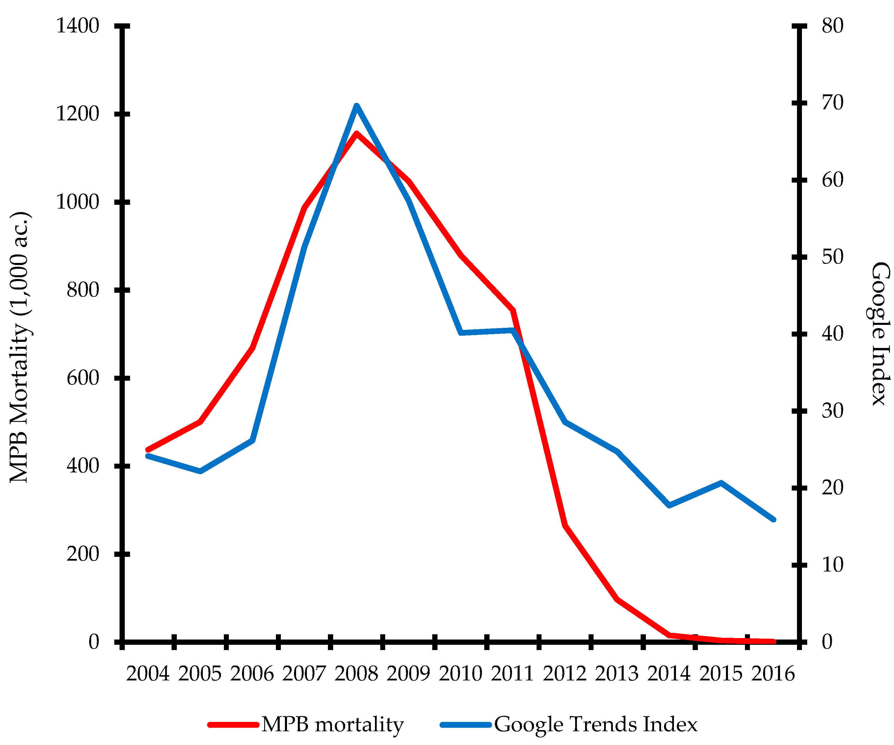
While traditional tools such as public surveys have been used to gauge the level of public awareness and sentiment regarding environmental threats, new tools such as Google Trends are being used to track changes in public interest regarding conservation topics [45]. A product of the Google search engine, Google Trends is a tool that returns the usage volume of a specific search term for specific locations over a defined period. While not the primary focus of the research reported here, it is hypothesized that public awareness and interest in the MPB outbreak was widespread throughout Colorado due to both its visibility across mountainous landscapes and the fact that this outbreak exceeded in areal extent any previous recorded outbreak.
As Google Trend data are recorded at monthly time steps, and as MPB mortality data are annual, Google Trend data were smoothed by computing annual average usage volume as the mean value over the monthly data for each year. This procedure provided a common basis for comparison of public awareness and interest with MPB outbreak severity.
A plot of the two-time trends (Appendix A Figure A1) indicates that public awareness of MPB in Colorado tracks very closely with the mortality levels. It is noted that public interest in the outbreak, as indicated by usage volumes, continued at relatively high levels even as the outbreak severity was rapidly diminishing. While it is not possible to detect the exact types of information that people were searching for, this result suggests that there was a residual effect of the outbreak as peoples’ lives continued to be affected during the aftermath of the outbreak.
Figure A1.
MPB mortality and public awareness in Colorado, 2004–2016.

References
- Vose, J.M.; Peterson, D.L.; Domke, G.M.; Fettig, C.J.; Joyce, L.A.; Keane, R.E.; Luce, C.J.; Prestemon, J.P.; Band, L.E.; Clark, J.S.; et al. Forests. In Impacts, Risks, and Adaptation in the United States: Fourth National Climate Assessment; Reidmiller, D.R., Avery, C.W., Easterling, D.R., Kunkel, K.E., Lewis, K.L.M., Maycock, T.K., Stewart, B.C., Eds.; U.S. Global Change Research Program: Washington, DC, USA, 2018; Volume 2. [Google Scholar]
- Dale, V.H.; Joyce, L.A.; McNulty, S.; Neilson, R.P.; Ayres, M.P.; Flannigan, M.D.; Hanson, P.J.; Irland, L.C.; Lugo, A.E.; Peterson, C.J.; et al. Climate change and forest disturbances. BioScience 2001, 51, 723–734. [Google Scholar] [CrossRef]
- Weed, A.S.; Ayres, M.P.; Hicke, J.A. Consequences of climate change for biotic disturbances in North American forests. Ecol. Monogr. 2013, 83, 441–470. [Google Scholar] [CrossRef]
- Breshears, D.D.; Cobb, N.S.; Rich, P.M.; Price, K.P.; Allen, C.D.; Balice, R.G.; Romme, W.H.; Kastens, J.H.; Floyd, M.L.; Belnap, J.; et al. Regional vegetation die-off in response to global-change-type drought. Proc. Natl. Acad. Sci. USA 2005, 102, 15144–15148. [Google Scholar] [CrossRef] [PubMed] [Green Version]
- Pile, L.S.; Meyer, M.D.; Rojas, R.; Roe, O.; Smith, M.T. Drought impacts and compounding mortality on forest trees in the southern Sierra Nevada. Forests 2019, 10, 237. [Google Scholar] [CrossRef]
- Radeloff, V.C.; Helmers, D.P.; Kramer, H.A.; Mockrin, M.H.; Alexandre, P.M.; Bar-Massada, A.; Bustic, V.; Hawbaker, T.J.; Martinuzzi, S.; Syphard, A.D.; et al. Rapid growth of the US wildland-urban interface raises wildfire risk. Proc. Natl. Acad. Sci. USA 2018, 115, 3314–3319. [Google Scholar] [CrossRef] [PubMed] [Green Version]
- Schelaas, M.-J.; Nabuurs, G.-J.; Schuck, A. Natural disturbances in the European forests in the 19th and 20th centuries. Glob. Chang. Biol. 2003, 9, 1620–1633. [Google Scholar] [CrossRef]
- Seidl, R.; Rammer, W.; Jäger, D.; Lexer, M.J. Impact of bark beetle (Ips typographus L.) disturbance on timber production and carbon sequestration in different management strategies under climate change. For. Ecol. Manag. 2008, 256, 209–220. [Google Scholar] [CrossRef]
- Seidl, R.; Schelhaas, M.-J.; Lexer, M.J. Unravelling the drivers of intensifying forest disturbances in Europe. Glob. Change Biol. 2011, 17, 2842–2852. [Google Scholar] [CrossRef]
- Ayres, M.P.; Lombadero, M.J. Forest pests and their management in the Anthropocene. Can. J. For. Res. 2018, 48, 292–301. [Google Scholar] [CrossRef] [Green Version]
- Morris, J.L.; Cottrell, S.; Fettig, C.J.; Sherriff, R.L.; Carter, V.A.; Clear, J.L.; Clement, J.; DeRose, R.J.; Hicke, J.A.; Higuera, P.E.; et al. Managing bark beetle impacts on ecosystems and society: Priority questions to motivate future research. J. Appl. Ecol. 2017, 54, 75–760. [Google Scholar] [CrossRef]
- Hodgson, D.; McDonald, J.L.; Hosken, D.J. What do you mean, ‘resilient’? Trends Ecol. Evol. 2015, 30, 503–506. [Google Scholar] [CrossRef] [PubMed]
- Millar, C.I.; Stephenson, N.L.; Stephens, S.L. Climate change and the forests of the future: Managing in the face of uncertainty. Ecol. Appl. 2007, 17, 2145–2151. [Google Scholar] [CrossRef] [PubMed]
- Holmes, T.P. Price and welfare effects of catastrophic forest damage from southern pine beetle epidemics. For. Sci. 1991, 37, 500–516. [Google Scholar]
- Pye, J.M.; Holmes, T.P.; Prestemon, J.P.; Wear, D.N. Economic impacts of the southern pine beetle. In Southern Pine Beetle II; Coulson, R.N., Klepzig, K.D., Eds.; General Technical Report SRS-140; USDA Forest Service Southern Research Station: Asheville, NC, USA, 2011. [Google Scholar]
- Patriquin, M.N.; Wellstead, A.M.; White, W.A. Beetles, trees, and people: Regional economic impact sensitivity and policy considerations related to the mountain pine beetle infestation in British Columbia, Canada. For. Policy Econ. 2007, 9, 938–946. [Google Scholar] [CrossRef]
- Hyde, K.; Peckham, S.; Holmes, T.; Ewers, B. Bark-beetle induced forest mortality in the North American Rocky Mountains. In Biological and Environmental Hazards, Risks, and Disasters; Shroder, J.F., Sivanpillai, R., Eds.; Elsevier: Amsterdam, The Netherlands, 2015. [Google Scholar]
- Michaelson, E. Economic impact of mountain pine beetle on outdoor recreation. South J. Agric. Econ. 1975, 7, 43–50. [Google Scholar] [CrossRef]
- Leuschner, W.A.; Young, R.L. Estimating the southern pine beetle’s impact on reservoir campsites. For. Sci. 1978, 24, 527–537. [Google Scholar]
- Price, J.I.; McCollum, D.W.; Berrens, R.P. Insect infestation and residential property values: A hedonic analysis of the mountain pine beetle epidemic. For. Policy Econ. 2010, 12, 415–422. [Google Scholar] [CrossRef]
- Cohen, J.; Blinn, C.E.; Boyle, K.J.; Holmes, T.P.; Moeltner, K. Hedonic valuation with translating amenities: Mountain pine beetles and host trees in the Colorado Front Range. Environ. Resour. Econ. 2016, 63, 613–642. [Google Scholar] [CrossRef]
- Taylor, L. Hedonics. In A Primer on Nonmarket Valuation; Champ, P.A., Boyle, K.J., Brown, T.C., Eds.; Springer: Dordrecht, The Netherlands, 2017. [Google Scholar]
- Van Praag, B.M.S.; Baarsma, B.E. Using happiness surveys to value intangibles: The case of airport noise. Econ. J. 2005, 115, 224–246. [Google Scholar] [CrossRef]
- Ferreira, S.; Mouro, M. On the use of subjective well-being data for environmental valuation. Environ. Resour. Econ. 2010, 46, 249–273. [Google Scholar] [CrossRef]
- Kahneman, D.; Wakker, P.P.; Sarin, R. Back to Bentham? Explorations of experienced utility. Q. J. Econ. 1997, 112, 375–405. [Google Scholar] [CrossRef]
- Frey, B.S.; Luechinger, S.; Stutzer, A. The life satisfaction approach to environmental valuation. Annu. Rev. Resour. Econ. 2010, 2, 139–160. [Google Scholar] [CrossRef]
- Jones, B.A. Invasive species impacts on human well-being using the life satisfaction index. Ecol. Econ. 2017, 134, 250–257. [Google Scholar] [CrossRef]
- USDA Forest Service. Areas with Tree Mortality from Bark Beetles: Summary for 2000–2017, Western US; Forest Health Protection: Fort Collins, CO, USA, 2013. Available online: https://www.fs.fed.us/foresthealth/applied-sciences/news/2018/wbb_summary.shtml (accessed on 12 August 2019).
- Kosiba, A.M.; Meigs, G.W.; Duncan, J.A.; Pontius, J.A.; Keeton, W.S.; Tait, E.R. Spatiotemporal patterns of forest damage and disturbance in the northeastern United States: 2000–2016. For. Ecol. Manag. 2018, 430, 94–104. [Google Scholar] [CrossRef]
- Coleman, T.W.; Graves, A.D.; Heath, Z.; Flowers, R.W.; Hanavan, R.P.; Cluck, D.R.; Ryerson, D. Accuracy of aerial detection surveys for mapping insect and disease disturbances in the United States. For. Ecol. Manag. 2018, 430, 321–326. [Google Scholar] [CrossRef]
- Meddens, A.J.H.; Hicke, J.A.; Ferguson, C.A. Spatiotemporal patterns of observed bark beetle-caused tree mortality in British Columbia and the western United States. Ecol. Appl. 2012, 22, 1876–1891. [Google Scholar] [CrossRef] [PubMed]
- Coulston, J.W.; Moisen, G.G.; Wilson, B.T.; Finco, M.V.; Cohen, W.B.; Brewer, C.K. Modeling percent tree canopy cover: A pilot study. Photogramm. Eng. Remote Sens. 2012, 78, 715–727. [Google Scholar] [CrossRef]
- Coulston, J.W.; Jacobs, D.M.; King, C.R.; Elmore, I.C. The influence of multi-season imagery on models of canopy cover: A case study. Photogramm. Eng. Remote Sens. 2013, 79, 469–477. [Google Scholar] [CrossRef]
- Levinson, A. Valuing public goods using happiness data: The case of air quality. J. Public Econ. 2012, 96, 869–880. [Google Scholar] [CrossRef]
- Thompson, M.T.; Shaw, J.D.; Witt, C.; Werstak, C.E.; Amacher, M.C.; Goeking, S.A.; DeRose, R.J.; Morgan, T.A.; Sorenson, C.B.; Hayes, S.W.; et al. Colorado’s Forest Resources, 2004–2013; Resource Bulletin RMRS-RB-23; USDA Forest Service Rocky Mountain Research Station: Fort Collins, CO, USA, 2017.
- Dolan, P.; Metcalfe, R. Comparing Willingness-To-Pay and Subjective-Well-Being in the Context of Non-Market Goods; Discussion Paper 890; Centre for Economic Performance, London School of Economics: London, UK, 2008. [Google Scholar]
- Ambrey, C.L.; Fleming, C.M. The causal effect of income on life satisfaction and the implications for valuing non-market goods. Econ. Lett. 2014, 123, 131–134. [Google Scholar] [CrossRef]
- Easterlin, R. Will raising the incomes of all increase the happiness of all? J. Econ. Behav. Organ. 1995, 27, 35–47. [Google Scholar] [CrossRef]
- Dolan, P.; Peasgood, T.; White, M. Do we really know what makes us happy? A review of the economic literature on the factors associated with subjective well-being. J. Econ. Psychol. 2008, 29, 94–122. [Google Scholar] [CrossRef]
- Zhang, X.; Zhang, X.; Chen, X. Happiness in the air: How does a dirty sky affect mental health and subjective well-being? J. Environ. Econ. Manag. 2017, 85, 81–94. [Google Scholar] [CrossRef] [PubMed]
- Holmes, T.P.; Adamowicz, W.L.; Carlsson, F. Choice experiments. In A Primer on Nonmarket Valuation; Champ, P.A., Boyle, K.J., Brown, T.C., Eds.; Springer: Berlin/Heidelberg, Germany, 2017. [Google Scholar]
- Smith, V.K. Reflections on the literature. Rev. Environ. Econ. Policy 2008, 2, 292–308. [Google Scholar] [CrossRef]
- Benjamin, D.J.; Kimball, M.S.; Heffetz, O.; Szembrot, N. Beyond happiness and satisfaction: Toward well-being indices based on stated preferences. Am. Econ. Rev. 2014, 104, 2698–2735. [Google Scholar] [CrossRef] [PubMed]
- Benjamin, D.J.; Cooper, K.B.; Heffetz, O.; Kimball, M. Challenges in constructing a survey-based well-being index. Am. Econ. Rev. 2017, 107, 81–85. [Google Scholar] [CrossRef] [PubMed]
- Proulx, R.; Massicotte, P.; Pépino, M. Googling trends in conservation biology. Conserv. Biol. 2013, 28, 44–51. [Google Scholar] [CrossRef] [PubMed]
Figure 1.
Forest mortality caused by Mountain Pine Beetle in Colorado counties.


Table 1.
Descriptive statistics.
| Variable | Variable Name | Mean | Std. Dev. | Min | Max |
|---|---|---|---|---|---|
| Life satisfaction | lsatisfy | 1.57 | 0.61 | 1 | 4 |
| Household income (ln) | ln_hhdinc | 10.69 | 0.71 | 8.52 | 11.32 |
| Married | married | 0.60 | 0.49 | 0 | 1 |
| Female | female | 0.60 | 0.49 | 0 | 1 |
| Employed | employed | 0.57 | 0.49 | 0 | 1 |
| Age | age | 53.51 | 16.10 | 18 | 99 |
| Age squared | age2 | 3123.03 | 1759.52 | 324 | 9801 |
| Education | educa | 5.05 | 1.01 | 1 | 6 |
| Excellent health | ex_health | 0.23 | 0.42 | 0 | 1 |
| Very good health | vg_health | 0.36 | 0.48 | 0 | 1 |
| Good health | gd_health | 0.27 | 0.44 | 0 | 1 |
| Fair health | fr_health | 0.10 | 0.30 | 0 | 1 |
| Boulder County mortality 1 | bold_mpb | 0.65 | 3.09 | 0 | 21 |
| Larimer County mortality 2 | lar_mpb | 1.46 | 7.30 | 0 | 57.8 |
| Grand County mortality 3 | gnd_mpb | 0.06 | 1.33 | 0 | 36 |
| Routt County mortality 4 | rou_mpb | 0.08 | 1.14 | 0 | 27.9 |
| Summit County mortality 5 | sum_mpb | 0.07 | 1.25 | 0 | 27.4 |
1 This variable is coded as zero for counties other than Boulder. Within Boulder County, average forest mortality = 12.25% during the study period. 2 This variable is coded as zero for counties other than Larimer. Within Larimer County, average forest mortality = 30.48% during the study period. 3 This variable is coded as zero for counties other than Grand. Within Grand County, average forest mortality = 25.31% during the study period. 4 This variable is coded as zero for counties other than Routt. Within Routt County, average forest mortality = 12.58% during the study period. 5 This variable is coded as zero for counties other than Summit. Within Summit County, average forest mortality = 18.4% during the study period.
Table 2.
Empirical results showing the impact of Mountain Pine Beetle (MPB) on life satisfaction for residents of Colorado counties.
Table 2.
Empirical results showing the impact of Mountain Pine Beetle (MPB) on life satisfaction for residents of Colorado counties.
| Variable | Coefficient | Standard Error | T-Statistic |
|---|---|---|---|
| ln_hhdinc | 0.119 *** | 0.009 | 13.55 |
| married | 0.179 *** | 0.007 | 24.77 |
| female | 0.035 *** | 0.006 | 5.47 |
| employed | 0.016 *** | 0.007 | 2.44 |
| age | −0.015 *** | 0.001 | 11.49 |
| age2 | 0.0002 *** | 0.00001 | 15.19 |
| educa | 0.001 | 0.004 | 0.24 |
| ex_health | 0.692 *** | 0.020 | 34.14 |
| vg_health | 0.538 *** | 0.021 | 25.28 |
| gd_health | 0.350 *** | 0.020 | 17.55 |
| fr_health | 0.199 *** | 0.022 | 8.88 |
| year2006 | 0.015 | 0.016 | 0.90 |
| year2007 | −0.010 | 0.018 | 0.55 |
| year2008 | 0.005 | 0.018 | 0.27 |
| year2009 | 0.011 | 0.020 | 0.57 |
| year2010 | 0.018 | 0.016 | 1.14 |
| bold_mpb | 0.002 *** | 0.001 | 2.80 |
| bold_mpb_lag1 | −0.003 *** | 0.001 | 3.54 |
| gnd_mpb | 0.033 *** | 0.001 | 46.80 |
| gnd_mpb_lag1 | -0.051 *** | 0.001 | 44.77 |
| lar_mpb | 0.0002 | 0.0005 | 0.41 |
| lar_mpb_lag1 | −0.0002 | 0.0005 | 0.35 |
| rou_mpb | 0.0001 | 0.0003 | 0.31 |
| rou_mpb_lag1 | −0.0026 *** | 0.0005 | 5.63 |
| sum_mpb | -0.002 *** | 0.0004 | 4.48 |
| sum_mpb_lag1 | -0.0022 *** | 0.0009 | 2.51 |
| constant | 3.223 *** | 0.098 | 33.01 |
| N | 40,388 | ||
| R2 | 0.17 |
Note: *** indicates significance at the 0.01 level. Also, for ease of interpretation, the signs of the parameter estimates reflect that the highest life satisfaction levels were coded as 4 and lowest life satisfaction levels were coded as 1.
Table 3.
Estimated change in life satisfaction, housing, and general forest characteristics for MPB counties in Colorado.
Table 3.
Estimated change in life satisfaction, housing, and general forest characteristics for MPB counties in Colorado.
| County | Δ in Life Satisfaction Index | Housing Units 1 | Total Forest Area (1000 ac) 2 | Pine Growing Stock, Net Volume (mm ft3) 2 | Av. Ann. Pine Net Growth (mm ft3) 2 |
|---|---|---|---|---|---|
| Boulder | −0.02 | 135,920 | 240.9 | 149.9 | 0.3 |
| Grand | −0.47 | 16,761 | 423.1 | 276.8 | −75.7 |
| Larimer | n.s. 3 | 148,549 | 345.5 | 522.2 | 0.8 |
| Routt | −0.03 | 16,839 | 443.7 | 287.6 | −21.8 |
| Summit | −0.08 | 31,106 | 114.5 | 151.5 | −7.4 |
1 US Census Bureau, 2018 data. 2 Thompson et al. [35]; Tables B32, B35, and B36. 3 n.s. indicates that parameter estimates were not statistically significant.
Table 4.
Comparison of per household monetized economic losses from forest mortality using Hedonic Method (HM) and Life Satisfaction Approach (LSA) estimates.
Table 4.
Comparison of per household monetized economic losses from forest mortality using Hedonic Method (HM) and Life Satisfaction Approach (LSA) estimates.
| County | Hedonic Model | Life Satisfaction Approach | Equilibrium 3 |
|---|---|---|---|
| Boulder | $61,000 1 | $8000 | No |
| Grand | n.a. 2 | $232,000 | No |
| Larimer | $76,000 1 | $0 | Yes |
| Routt | n.a. 2 | $18,000 | No |
| Summit | n.a. 2 | $44,000 | No |
1 Estimates provided in [16]. Economic losses in this study reflect differences in price for homes located within host tree zones versus homes located outside of host tree zones. 2 n.a indicates estimates are not available. 3 Based on LSA results, is the housing market in equilibrium after the MPB outbreak?
© 2019 by the authors. Licensee MDPI, Basel, Switzerland. This article is an open access article distributed under the terms and conditions of the Creative Commons Attribution (CC BY) license (http://creativecommons.org/licenses/by/4.0/).
Share and Cite
MDPI and ACS Style
Holmes, T.; Koch, F. Bark Beetle Epidemics, Life Satisfaction, and Economic Well-Being. Forests 2019, 10, 696. https://doi.org/10.3390/f10080696
AMA Style
Holmes T, Koch F. Bark Beetle Epidemics, Life Satisfaction, and Economic Well-Being. Forests. 2019; 10(8):696. https://doi.org/10.3390/f10080696
Chicago/Turabian StyleHolmes, Thomas, and Frank Koch. 2019. "Bark Beetle Epidemics, Life Satisfaction, and Economic Well-Being" Forests 10, no. 8: 696. https://doi.org/10.3390/f10080696
Note that from the first issue of 2016, this journal uses article numbers instead of page numbers. See further details here.