How Well Do Stakeholder-Defined Forest Management Scenarios Balance Economic and Ecological Forest Values?


1
Department of Forest Resource Management, Swedish University of Agricultural Sciences, Skogsmarksgränd, 90183 Umeå, Sweden
2
Natural Resources Institute Finland, Latokartanonkaari 9, 00790 Helsinki, Finland
3
Swedish Species Information Centre, Swedish University of Agricultural Sciences, Box 7070, 75007 Uppsala, Sweden
*
Author to whom correspondence should be addressed.
Forests 2020, 11(1), 86; https://doi.org/10.3390/f11010086
Submission received: 7 November 2019
/
Revised: 9 December 2019
/
Accepted: 28 December 2019
/
Published: 9 January 2020
(This article belongs to the Section Forest Economics, Policy, and Social Science)
Abstract
:Research Highlights: We show the difference in the long-term effects on economic and ecological forest values between four forest management scenarios of a large representative forest landscape. The scenarios were largely formulated by stakeholders representing the main views on how to manage north-European forests. Background and Objectives: Views on how to balance forest management between wood production and biodiversity differ widely between different stakeholder groups. We aim to show the long-term consequences of stakeholder-defined management scenarios, in terms of ecological and economic forest values. Materials and Methods: We simulated management scenarios for a forest landscape in Sweden, based on the management objectives and strategies of key stakeholders. We specifically investigated the difference in economic forest values coupled to wood supply and ecological indicators coupled to structural biodiversity between the scenarios over a 100-year period. The indicators were net present value, harvest, growing stock and increment, along with deadwood volume, the density of large trees, area of old forests and mature broadleaf-rich forests. Results: We show that the scenarios have widely different outcomes in terms of the studied indicators, and that differences in indicator outcome were largely due to different distributions in management regimes, i.e., the proportion of forest left unmanaged or under even-aged management or continuous cover forest, as well as specific retention practices. Retention and continuous cover forestry mitigate the negative effects that clear-cut forestry has upon biodiversity. Conclusions: We found that an increase in the forest area under the continuous cover forestry regime could be a cost-efficient way to increase structural diversity in managed boreal forests. On the other hand, no single management regime performed best with respect to all indicators, which means that a mixture of several management regimes is needed to balance conflicting objectives. We also show that the trade-off between economic and ecological indicators was not directly proportional, meaning that an increase in structural biodiversity may be obtained at a proportionally low cost with appropriate management planning.
1. Introduction
More than half of the world’s forests are managed for wood production, often in combination with other uses [1]. Globally, wood harvesting has increased during the last decades [2]. Climate change mitigation efforts and the transition to a bio-based economy are likely to further increase the demand for wood products, both for material use and energy production [3,4]. Forest management for wood production has a net negative impact on biodiversity [5]. However, management regimes differ widely in their impact upon biodiversity [6], suggesting that the conflict between wood production and biodiversity conservation can be alleviated by well-informed management decisions.
There is still limited knowledge on how forest management can help to reduce the trade-off between wood production and biodiversity conservation in the long term, and views on how to manage the forest differ widely between different stakeholder groups [7,8,9]. A frequently used approach to investigate the consequences of forest management on the long-term development of forest resources, associated ecosystem services and biodiversity, is quantitative scenario analysis using forest decision support systems [10,11]. Scenarios are powerful tools to envision how forest ecosystems may respond to different driving forces and management options [10,12]. However, scenario analysis in and of itself does not explore how stakeholders and decision-makers perceive the importance of a variety of criteria in relation to different forest values. The integration of stakeholders (groups or individuals affecting or affected by the management) in scenario development is beneficial, as it encourages a better consideration of differing values, interests and transdisciplinary knowledge than pure academic scenarios [13,14,15,16]. However, participatory approaches, where realistic and possibly implementable scenarios addressing forest management are investigated, are rare [10]. This is unfortunate as recent examples exist of the successful implementation of forest decision support tools in participatory settings for supporting stakeholder negotiations [17,18,19].
The conflict between wood production and biodiversity is acute in Fennoscandian forests. Even-aged forest management, with clear-cut harvesting and thinning from below, has been the dominant management regime in Fennoscandia since World War II [20]. Industrial-scale, clear-cut harvesting has turned Fennoscandia into a key wood provider at the global level. For example, despite holding less than one percent of the world’s commercial forests, Sweden is the world’s third largest exporter of pulp, paper and sawn timber [21]. At the same time, intensive clear-cut forestry is a major reason for the red-listing of Fennoscandian species [22,23,24]. However, international agreements such as the Convention on Biological Diversity and the European Union (EU) Biodiversity Strategy 2014, as well as national environmental quality objectives state that biodiversity shall be preserved. Legally protected areas alone cannot ensure the long-term persistence of species [25]. This means that there is a need to start identifying alternative management strategies that are effective in preserving biodiversity [6], while still meeting the forest owners’ economic expectations from their forests [26,27], and the increasing wood demand that a transition to a bio-based economy is expected to require [28].
As a response to the rapid transformation and simplification of forests that industrial-scale clear-cut harvesting regimes entail, retention forestry emerged about 30 years ago in North America, and is becoming increasingly common in forestry globally [29,30]. In retention forestry, single living or dead trees, tree patches and buffer strips are left unlogged, in order to increase structural and compositional diversity, to provide stepping-stones, and to support the life-boating of species between forest generations [31,32]. This has been shown to moderate the effects of pure clear-cuts [33,34,35]. Lindenmayer et al. [36] even suggested spreading retention forestry over the globe to stop the decline of biodiversity. As retention forestry has only been practiced for a few decades, knowledge on its long-term effects, i.e., covering a whole forest rotation or more, can only be derived from simulation studies.
Another management regime that has received increasing attention during recent years is continuous cover forestry (CCF), a silvicultural regime without a clear-cut phase [20,37,38]. It is an old forest management method in Europe [39], and is also considered to better maintain late-successional forest characteristics and species assemblages than even-aged management [20].
CCF meets diverse management objectives and the provision of more ecosystem services related to a continuous forest cover [38,40,41,42,43,44]. In CCF, forests are harvested by selection felling or by creating small gaps to enable natural regeneration and an uneven-aged forest structure.
Other measures that have been brought up in recent years, aiming at increasing structural diversity and thus maintaining biodiversity, include longer rotation periods, promoting broadleaves, and increasing the proportion of the area that is set aside from forestry [7]. While there is a general agreement, also reflected in the Swedish forest legislation, that forestry should both produce wood and maintain biodiversity, there are widely differing views on how to reach that goal among stakeholders.
In this study, we aim to show the difference in the long-term effects of economic and ecological forest values between a set of stakeholder-defined management scenarios of a boreal forest landscape. More specifically, we ask:
- What is the difference between the stakeholder scenarios in terms of indicators for economic forest values coupled to wood supply and structural biodiversity indicators?
- What is the contribution of different management regimes and retention practices to the differences in the economic and ecological indicators?
- What are our management recommendations aiming at balancing economic and ecological forest values based on the scenario results?
The scenarios are long-term (100 years), and cover an area of more than 100,000 ha of boreal forest in Sweden. The stakeholder scenarios were developed using a participatory approach, integrating the forest management and conservation interests of four key stakeholders. The stakeholders—which include Sweden’s largest forest owner, governmental agencies, as well as non-governmental organizations—have large impact upon forest biomass production and conservation in the area, and represent both economic and ecological interests.
2. Materials and Methods
2.1. Study Landscape
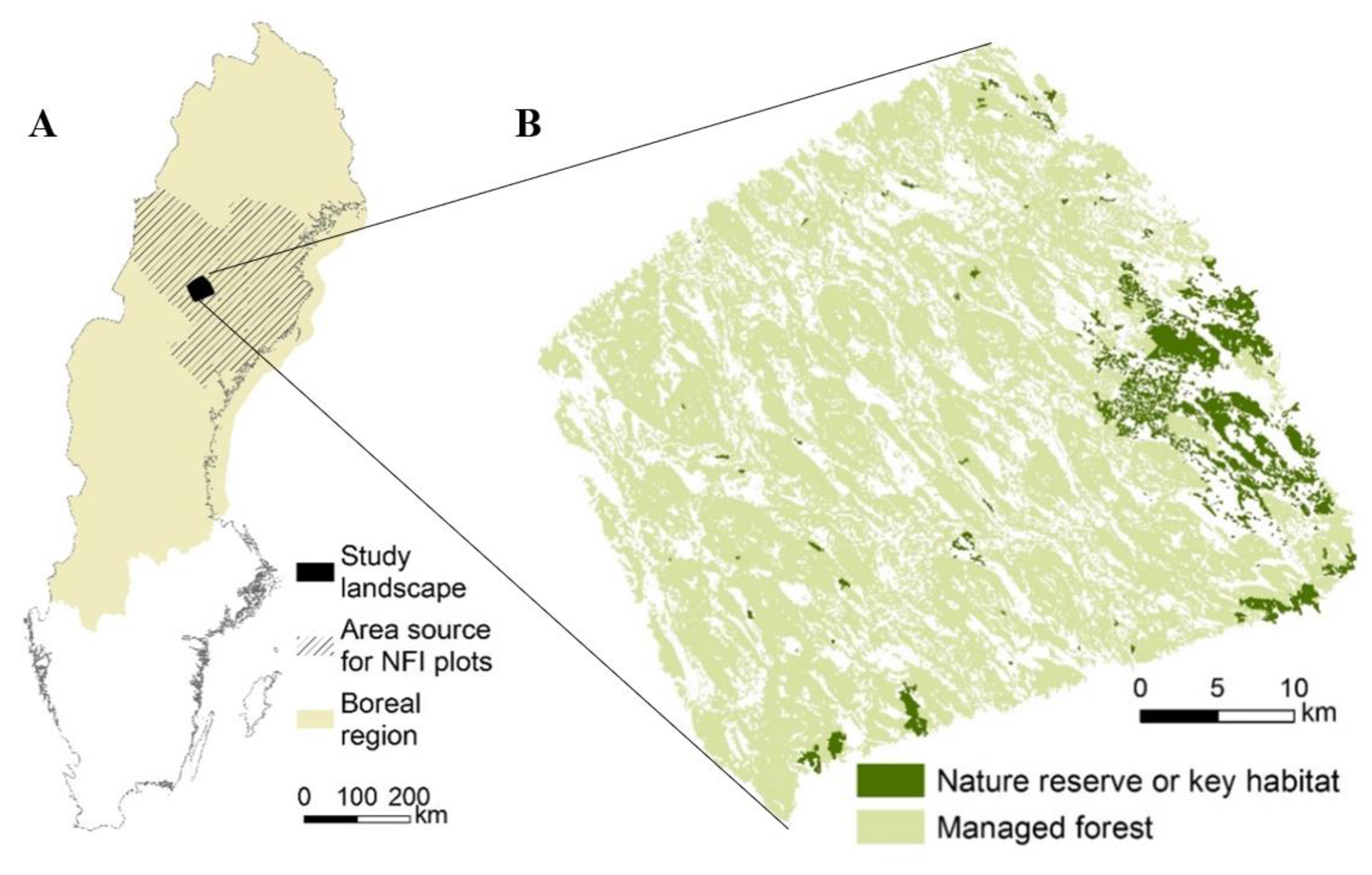
The study landscape is located in the middle of the boreal region in northern Sweden (Figure 1). Input data for the scenario projections were based on a segmented country-wide forest map [45], which provided stand boundaries. We combined the stand boundaries with spatial information on land cover, protected forest areas and key habitats, and then allocated data on forest stand conditions from National Forest Inventory (NFI) plots to the stands (see Appendix A for more information). The NFI plot data are from the years 2008–2012, and thus they describe, on average, the state of the forest in 2010. We chose NFI plots that are representative of forest conditions in middle boreal Sweden (Figure 1), in terms of productivity, tree species and age class distribution. Choosing NFI plots from a larger region ensured a larger variation in the initial forest conditions, as the number of NFI plots located within our study area is less than 100.
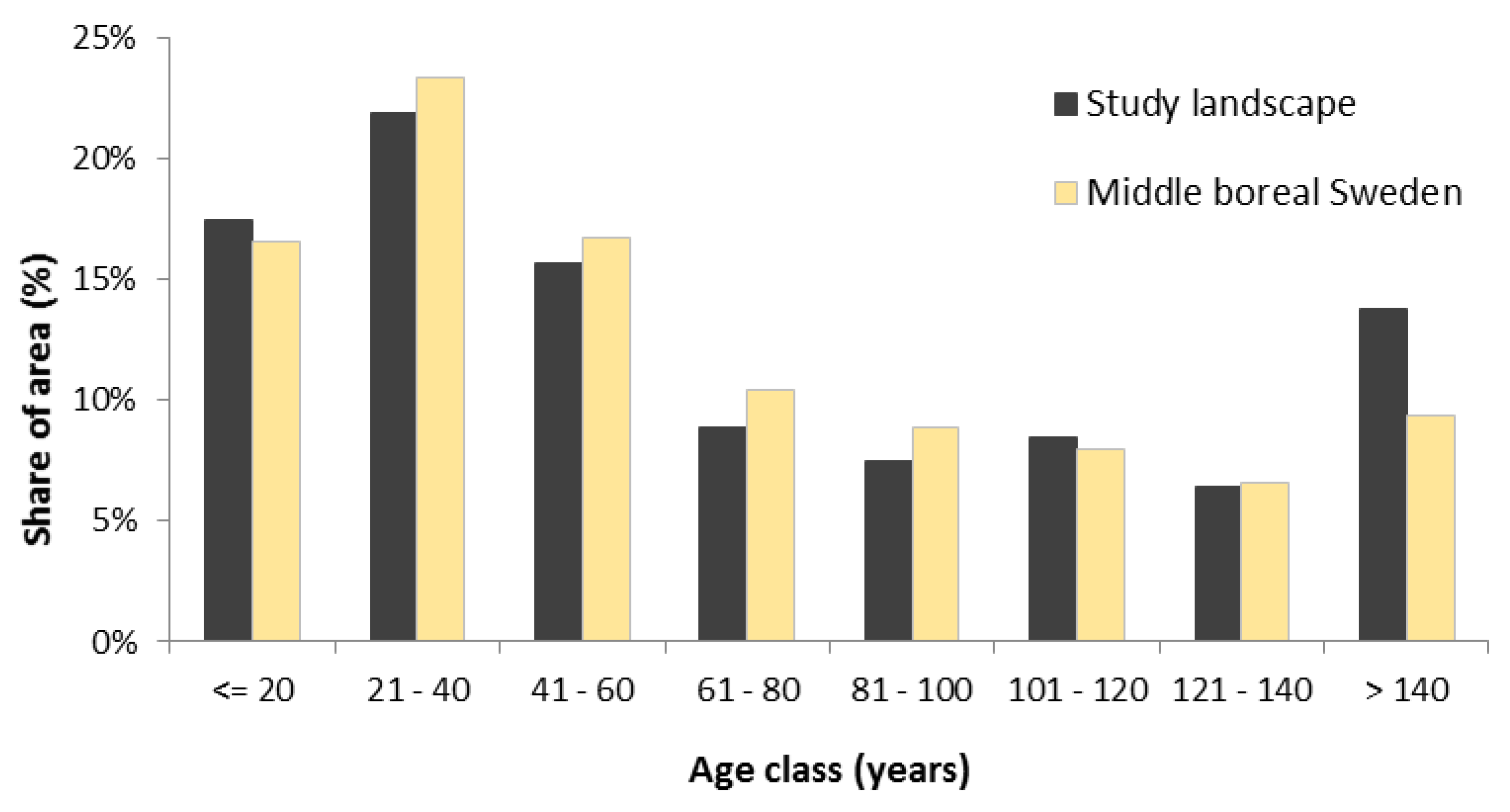
The study landscape comprised 103,313 ha of productive boreal forest, divided into 10,782 forest stands. Productive forest was defined as forest with a mean growth larger than 1 m3/ha/year. The forest was dominated by conifers, and the growing stock was distributed into Pinus sylvestris 40%, Picea abies 42%, Betula ssp. 16%, Populus tremula 0.4% and other broadleaves 1.3%. The mean age was 72 years, with the majority of the forest, 55%, being younger than 60 years (Figure 2). 7.8% of the forest area was located in nature reserves or classified as woodland key habitat, i.e., stands where red-listed species could be expected to occur [46], and which we assume are permanently set-aside from forestry.
2.2. Simulation and Optimization of Forest Dynamics and Management
The forest management scenarios were simulated using the PlanWise application of the Heureka forest decision support system, which includes a built-in optimization tool [47]. The core of the Heureka system consists of a set of empirical growth and yield models that project the tree layer development in 5-year time steps. The models were developed by means of regression analysis using data from the National Forest Inventory, long-term experiments, and yield plots, and they include models for stand establishment, diameter growth, height growth, tree recruitment and mortality [48,49,50].
In PlanWise, projections of future forest conditions are made in two steps: treatment simulation and then treatment selection. First, a set of alternative treatment schedules is created for each stand for one or several management strategies. A treatment schedule is a sequence of treatments, such as thinnings and final fellings during the planning horizon, here 100 years.
Management strategies are user-defined sets of silvicultural options and can differ in management regime (unmanaged, even-aged or uneven-aged), silvicultural practices (e.g., regeneration type, regeneration species, thinning type and intensity) and retention practices within stands (size of retention patches, number of retention trees and high stumps (stems cut 4 m above ground during a felling operation to increase the availability of deadwood) left in the final felling). For a given management strategy, several treatment schedules are created, differing in the timing of the treatments. For each stand and all its treatment schedules, a large number of variables describing the tree layer is calculated through time, including harvest volume and forest stand structure indices. Also, the net present value (NPV) is calculated, defined as the sum of discounted revenues minus the costs of forest management activities for an infinite time horizon. Second, in the treatment selection step, each stand is assigned the treatment schedule that minimizes or maximizes a user-defined objective function (e.g., NPV) and fulfils a set of user-defined constraints, using a mixed integer optimization model.
2.3. Participating Stakeholders
The following stakeholders were included: the branch organization LRF Skogsägarna, representing >100,000 private land owners managing >25% of the total forest land in Sweden (LRF); Sweden’s largest forest owner, state-owned Sveaskog, managing 15% of the productive forest land in Sweden (SVEA); the Swedish Society for Nature Conservation (SSNC), a non-governmental organization, with 226,000 members and a century-long tradition of working for forest conservation; and the Swedish Environmental Protection Agency (SEPA), working with all of the agencies having responsibilities within the Swedish Environmental Quality Objectives system, and responsible for following up and evaluating several of the Swedish Environmental Quality Objectives. The stakeholders have a large impact upon forest management and conservation in Sweden, either by managing a large share of the forest (SVEA), by lobbying for private landowners’ interests (LRF), by developing and implementing environmental policy (SEPA), or by lobbying for nature conservation (SSNC). Another stakeholder, the Swedish Forest Agency, which is responsible for operationalizing the national forest policy goals, and for the Environmental Quality Objective “Sustainable Forests”, actively participated in the scenario formulation discussions, but without defining a separate scenario. One to two representatives of each stakeholder organization participated in a series of stakeholder workshops (September 2016, October 2017, April 2018, and December 2018). Additionally, the researchers had email conversations with the individual stakeholder representatives in between workshops to discuss scenario-specific issues.
2.4. Stakeholders’ Forest Management Scenarios
All participating stakeholders were asked to describe how they would like the forest in the study landscape to be managed, and which targets they want to achieve. This included, for example, how much of the forest area should be set aside with no management, distribution of management regimes (even-aged or uneven-aged), regeneration practices (plantation or natural regeneration) and targets for deadwood volumes or the proportion of broadleaved trees. In addition, stakeholders were given the opportunity to modify their scenario specification upon the presentation of preliminary results. This resulted, however, only in minor additions to scenario specifications. The final scenario descriptions were used to create four management scenarios differing in the distribution of management regimes, the applied management strategies, as well as the constraints defined in the optimization model (Table 1).
In all four scenarios, the study landscape was first divided into both reserves and the forest available for wood supply (production forest) (Table 2). Reserves were left unmanaged. The extent and location of the reserve area was based on stakeholder specification and varied between scenarios, but always included nature reserves and key habitats (7.8% of the forest area). In all but the LRF scenario, additional stands were chosen to be included in the reserve category, based on a biodiversity index (i.e., prioritizing stands with a high biodiversity index) [51].
For the production forest, we defined several different management strategies for which treatment schedules were created, based on the aims and targets defined by the stakeholders. Management strategies included different options for even-aged and uneven-aged forest management with varying amounts of tree retention.
Even-aged forest management in our study landscape typically involves the following: soil scarification, planting or natural regeneration with seed trees, pre-commercial thinning (cleaning) at the height of 2–5 m, one or two thinnings with about 30% removal of the volume at each instance, and final felling after the lowest allowable final felling age, with or without leaving seed trees. Even-aged management strategies differed in the type of regeneration (planting, seed trees or shelterwood), the proportion of plantations with genetically improved seedlings, the proportion of broadleaves retained during cleanings and thinnings and rotation length.
Uneven-aged management was applied only for spruce-dominated forests and included strategies for continuous cover forestry (CCF). CCF is implemented as a continual series of selection fellings, which are simulated as thinning from above, i.e., harvesting of the largest trees. Models for natural regeneration are used to simulate tree recruitment. The stand is never clear-felled, and acquires an uneven age–class distribution over time.
Retention forestry is simulated by leaving a user-defined number of retention trees and high stumps on the final felling site, and by setting-aside a user-defined proportion of the stand as a retention patch. Retention patches are created in the beginning of the simulation, and at that point they have the same relative properties as the remaining stand. Retention patches are treated with selection felling when the parent stand is thinned or final felled.
While the overall retention efforts—in terms of number of retention trees, high stumps and size of retention patches—varied between scenarios (Table 1), retention always included a 15 m buffer zone around open water.
Not all management strategies were simulated for all stakeholders. LRF and SVEA did not choose to include alternative management strategies, so we included only even-aged management options for these stakeholders. This reflects current management practices in Sweden. SSNC and SEPA asked for a larger variation in management, and we included the CCF of spruce-dominated forests, shelterwood management of stands not dominated by spruce, and mixed-species, even-aged management, in which a 40% share of broadleaves is retained during cleanings and thinnings (instead of the commonly practiced broadleaf admixture of 10%–15%).
We used timber and pulpwood prices based on 2017 price levels for our study area and typical management costs based on the analysis of forest management practices (e.g., [52,53]). Costs and prices per volume unit were assumed to be constant over time.
In the optimization, NPV was maximized in all four scenarios, using a discount rate of 2.5%. Several stakeholder-specific forestry targets were implemented as constraints in the optimization model, such as the share of forest area under CCF and shelterwood management, evenness constraints for harvest volumes and revenues, as well as targets on deadwood and broadleaf volumes (Table 1 and Appendix B). Each unit of area was set to follow its allocated strategy throughout the whole planning period. The models were formulated and solved within the Heureka PlanWise system using the ZIMPL optimization language [54] and Gurobi 7.0, using a traditional branch and bound algorithm with a convergence bound of 0.01%.
2.5. Economic and Ecological Indicators
We compared the scenario outcomes for a set of indicators for economic forest values coupled to wood supply, and ecological forest values based on structural biodiversity indicators.
The main marketed ecosystem service of Swedish forests is timber production. Therefore, we used harvest volume, NPV, net growth and growing stock as economic indicators.
Harvest volume is a measure of wood supply, while net growth and growing stock are measures for the future potential of wood supply. NPV is a measure of the economic profitability of wood production. The economic indicators were calculated only for the production forest, because the wood in reserves is not available for the markets.
The ecological indicators were the density of large trees, proportion of old forest, deadwood volume and the proportion of mature forest with a high share of broadleaves. Large trees are amongst the most important substrates for red-listed species in boreal forests [55]. In boreal old-growth forests with natural fire regimes, it was probably common to have at least 20 trees per ha with a diameter at breast height (dbh) of at least 40 cm, which can be compared to the present value of around one such tree per ha in intensively managed Swedish forests [56]. The volume of dead wood in managed forests is a critical factor in their ability to retain forest specialist species [57]. In Sweden, the average volume of dead wood in managed forests is 7.6 m3/ha, whereas a volume of 20–30 m3/ha has been suggested as threshold for the biodiversity conservation in boreal coniferous forests [58]. The area of old forest, mature forest with a high proportion of broadleaves and deadwood quantity, are used as indicators to follow up the Swedish environmental quality objective “Sustainable Forests” [59].
3. Results
3.1. Forest Management
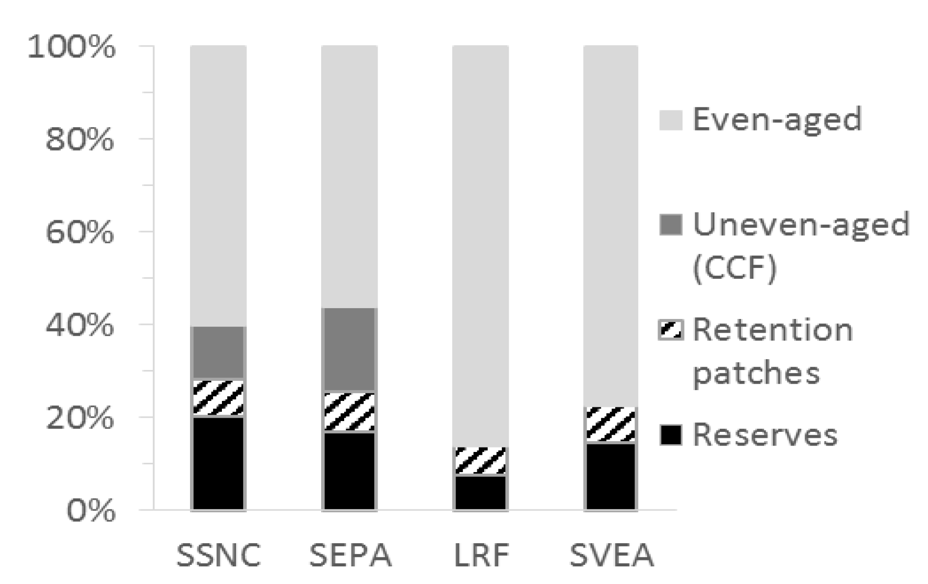
The four stakeholder scenarios varied considerably in the proportion of area under different management regimes (Figure 3). The proportion of unmanaged forests, or forests managed for nature conservation (nature reserves, key habitats and retention patches) varied between 15% (LRF) and 28% (SSNC), and the proportion of even-aged management varied between 22% (SEPA) and 85% (LRF). CCF was only applied in two of the scenarios (SSNC and SEPA).
3.2. Economic Indicators
NPV was highest in the LRF and SVEA scenarios, and approximately 14% lower in the SSNC and SEPA scenarios (Table 3). These differences are partly due to the varying proportions of reserves in the scenarios—differences in NPV are smaller when comparing the NPV for the production forest only.
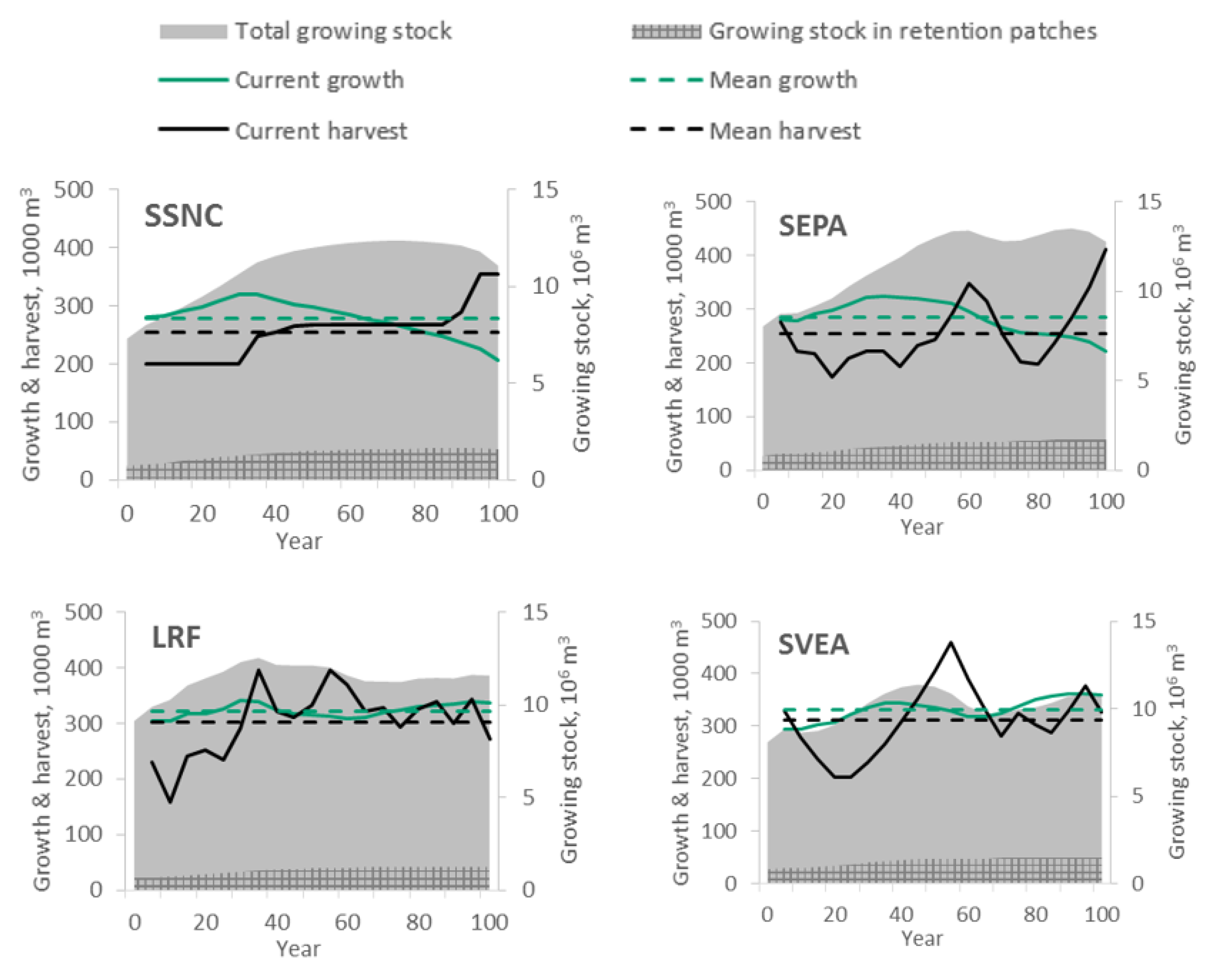
The net growth of wood increased initially in all four scenarios (Figure 4). This continued in the SVEA scenario for most of the simulation period, while growth remained relatively stable in the LRF scenario, but started to decrease after about 30 years in the SSNC and SEPA scenarios. The differences in growth were mainly caused by differences between scenarios in the area of managed forest (the lower the managed area, the lower growth), the proportion of management regimes, regeneration settings (plants from tree-breeding programs promote future growth compared to natural regeneration) and rotation lengths in the even-aged management regime.
In total, harvest volume was highest in the SVEA and LRF scenarios, with a mean annual harvest of more than 300,000 m3, and approximately 20% lower in the SSNC and SEPA scenarios. Harvest patterns varied between scenarios (Figure 4), due to constraints set in the optimization (Table 2). In SSNC, with a constraint of non-decreasing harvest flows, the harvest volume increased over time. However, as growth decreased over time, and the harvest exceeded growth during the last 30 years, this harvest level is not sustainable after the end of the simulation period. All other scenarios allowed for a decrease in harvest volume over time, only limiting deviations between consecutive periods.
At the end of the 100-year simulation period, the growing stock of production forests was higher than the initial growing stock in all scenarios, with the largest increase in the SEPA scenario. However, in all scenarios, harvest volumes exceeded growth at times, leading to a temporary decrease in growing stock.
CCF led to lower mean annual harvest and growth, but a higher standing volume and larger NPV compared with forests managed with even-aged management (Table 4). This is caused by a decrease in harvest volume over time in forests managed with CCF, while harvest volumes increased in forests under even-aged management.
3.3. Ecological Indicators
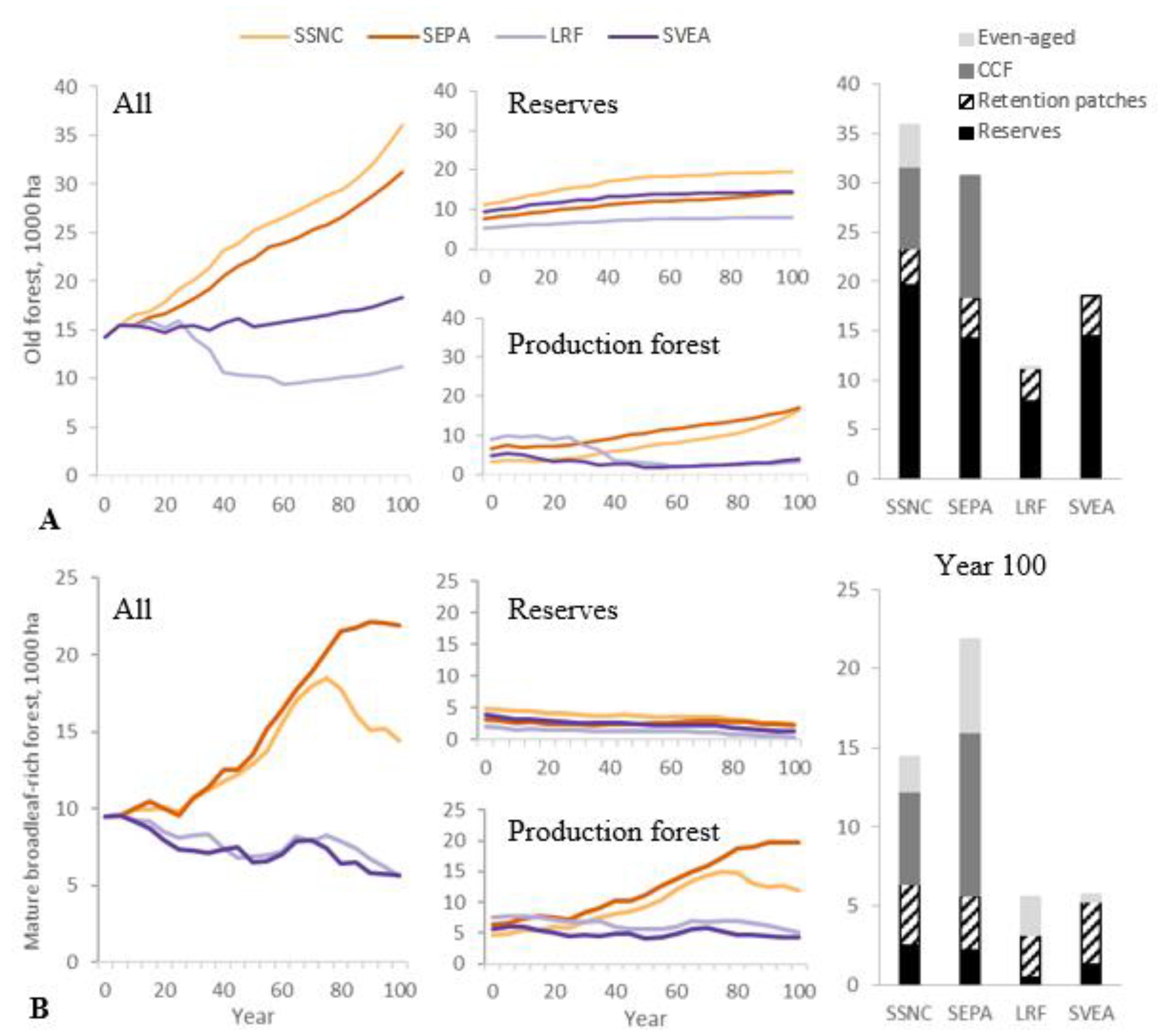
The scenarios resulted in large differences in all ecological indicators over time (Figure 5 and Figure 6). The SSNC and SEPA scenarios consistently resulted in higher indicator values compared to the LRF and SVEA scenarios. Deadwood volumes and the number of large-diameter trees increased in all scenarios, but at different levels. The area of old forest and mature broadleaf-rich forest, on the other hand, decreased or remained stable over time for the LRF and SVEA scenarios, while it increased in the SSNC and SEPA scenarios.
The differences in old forest area were to a large part due to divergent development in the production forest, where an increasing proportion of the forest managed with the CCF in the SSNC and SEPA scenarios counted as old forest over time (Figure 5A). This led to an increase in the proportion of old forest in the production forest in these scenarios, while its proportion decreased in the LRF and SVEA scenarios, which did not include CCF. After 100 years, old forest was almost non-existing in forests under even-aged management. Only the SSNC scenario, which required at least 20% of the managed forest to be older than 140 years in the end of the simulation (Table 2), had a non-negligible proportion of old forest area in the even-aged management regime.
The proportion of mature broadleaf-rich forest increased from the initial 9% in the SSNC and SEPA scenarios, but decreased in the other two scenarios (Figure 5B). In SSNC, the proportion started to decrease towards the end of the simulation period, mostly due to a decrease of this forest type in forests under even-aged management. In protected forests, the proportion of mature broadleaf-rich forests decreased over time in all scenarios. Thus, the smaller proportion of mature broadleaf-rich forest in the LRF and SVEA scenarios, compared to the SSNC and SEPA scenarios, was largely due to a lack of the CCF regime in LRF and SVEA.
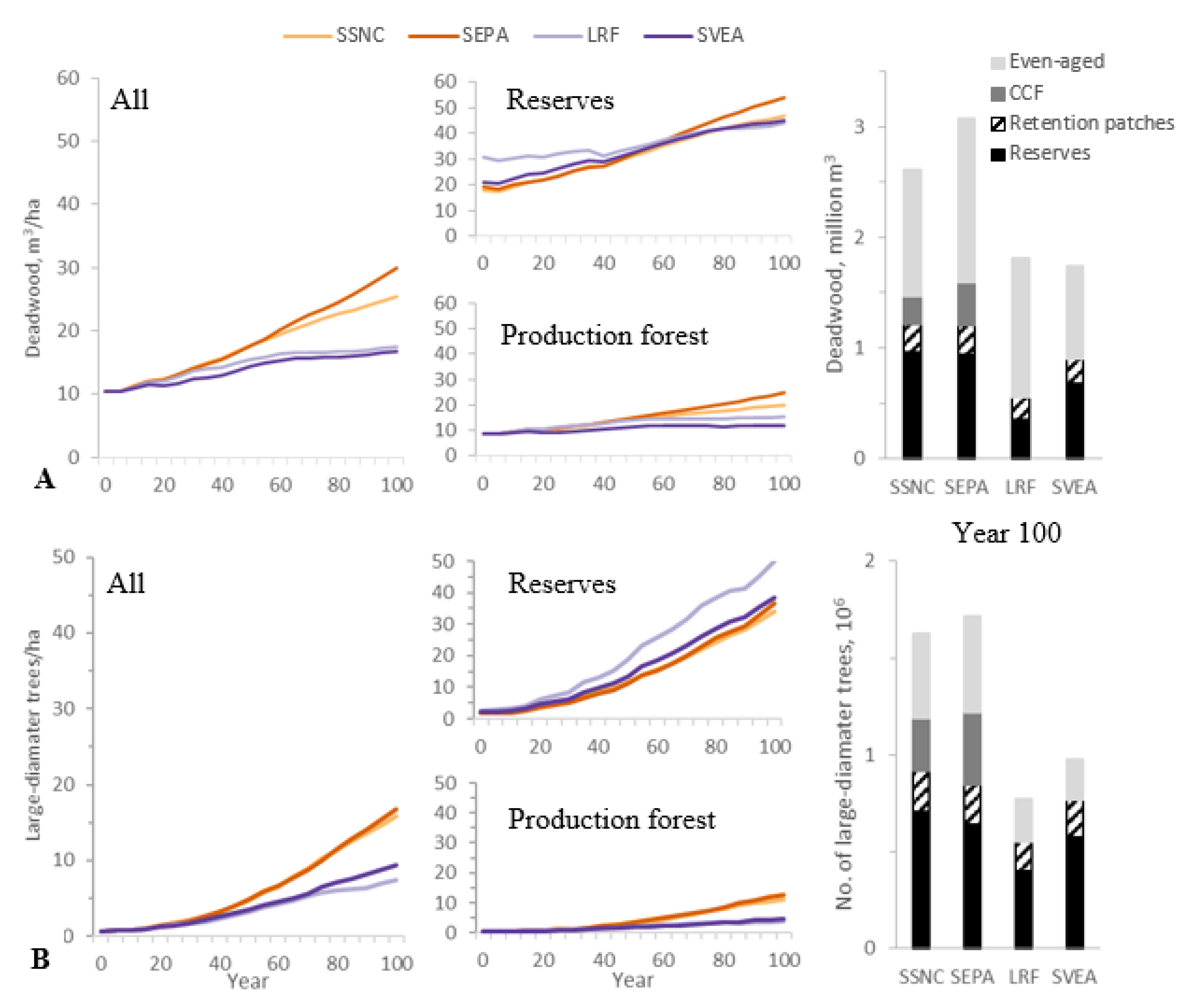
Deadwood volumes increased over time in all stakeholder scenarios, both in reserves and in the production forest (Figure 6A). The increase was largest in the SEPA and SSNC scenarios, and smallest in the LRF and SVEA scenarios. In the beginning, the LRF scenario had the highest average deadwood volume in reserves, as only existing nature reserves and key habitats were set aside from forest management. In the other scenarios, new reserves were created by setting aside additional forest stands until the target for reserve area was reached (see Appendix B). These stands had, on average, lower deadwood volume compared to existing reserves.
The average density of large-diameter trees, i.e., trees with a dbh of at least 40 cm, increased considerably in all scenarios (Figure 6B), from initially less than 1 tree/ha to around 16 (SSNC and SEPA), 7 (LRF) and 9 (SVEA) over the course of 100 years. After 100 years, the large-diameter tree density was highest in protected areas, and lowest in forests managed with even-aged forestry (Table 5). However, in the end of the simulation, the average number of large-diameter trees in forests under the even-aged management regime was comparable to the current levels in reserves in our study landscape (around 2.7 or less trees with dbh ≥ 40 cm per ha, depending on the scenario). This increase was mainly due to retention practices, as a minimum of eight solitary retention trees per ha were left during the final fellings in all scenarios, in addition to the setting aside of retention patches.
In the end of the simulation, the main explanation for difference in indicator values between the scenarios was the different management regimes, in particular the proportion of reserves, CCF and retention patches, which was more important compared to varying silvicultural details within even-aged management. (Table 5). Particularly in reserves, the area of old forest, deadwood and the density of large trees were high, while the proportion of mature broadleaf-rich forests was highest in forests managed with CCF and in retention patches.
In the production forest, even-aged management resulted in considerably lower ecological indicator values compared to CCF and retention patches, even though management strategies varied considerably for the even-aged management regime between stakeholders.
3.4. Integrative Assessment
The SSNC and SEPA scenarios led to higher levels for the ecological indicators, while the LRF and SVEA scenarios led to higher levels for the economic indicators (Table 6). The variation in indicator levels between scenarios was generally higher for the ecological indicators than for the economic indicators, indicating that increases in structural biodiversity are not necessarily proportional to losses in economic forest values. The variation in ecological indicator levels was particularly large for old and mature broadleaf-rich forest.
4. Discussion
In this study, we developed stakeholder-defined forest management scenarios and compared their long-term effects on the indicators of economic and ecological forest values. The scenarios aimed to build knowledge on the long-term impact of stakeholder-defined management prescriptions on wood production and conservation, rather than finding a compromise scenario that balances the objectives of all stakeholders. We show that the scenarios have widely different outcomes in terms of the studied indicators, and that differences in indicator outcome between scenarios were largely due to different distributions in management regimes between the scenarios.
All the stakeholders had multiple objectives, including wood production and the conservation of biodiversity, even though the focus of interest differed. The LRF and SVEA scenarios largely reflect current management practices. Even though wood production and biodiversity protection are co-equal goals in the Swedish forestry legislation, current management practices favour wood production [7,60]. The SSNC and SEPA scenarios, on the other hand, have a stronger focus on biodiversity protection, which is also reflected in the results. The SSNC and SEPA scenarios generally led to higher future levels for the ecological indicators, while the LRF and SVEA scenarios resulted in higher levels for the economic indicators, confirming that there is a clear trade-off between economic and ecological forest values. The difference in economic indicator outcome between scenarios is partly explained by the difference in reserve area between scenarios, with a smaller variation in NPV per ha when comparing only the production forest rather than the total forest area.
The overall difference between scenarios for the ecological indicators was larger than the overall difference between the economic indicators among the scenarios formulated by stakeholders with widely different views on forest use. This means that an increase in structural biodiversity is not necessarily directly proportional to a decrease in economic values coupled to wood supply. Hence, an increase in structural biodiversity may be obtained at a proportionally lower cost with appropriate management planning. However, there may be other, more effective ways to reduce the trade-off between wood production and biodiversity than the stakeholder scenarios suggest. Previous research has shown that a combination of different management strategies is needed to resolve conflicts between conflicting objectives [7,9], and that a variation in management strategies (i.e., more site-adapted management) can be more profitable than just applying a single strategy to all stands [61]. Therefore, adding more variation to, for example, the SVEA scenario, may result in both higher economic and ecological indicator outcomes for this scenario.
While the proportion of old and mature-broadleaf-rich forest remained stable or decreased in LRF and SVEA, but increased in SSNC and SEPA, deadwood volumes and the density of large trees increased considerably in all scenarios, compared to initial conditions. However, this was from a very low initial level, which is the result of decades of intensive forest management. In particular, large diameter trees are very rare in today’s Fennoscandian forests, and our simulation results suggest that their numbers will increase dramatically in the future, both in reserves, and to a lesser extent, in production forests. The overall increase was particularly pronounced in the SEPA and SSNC scenarios. Average deadwood volumes increased considerably over the course of the 100-year simulation period, in all scenarios. After 100 years, forests outside reserves had an average deadwood volume above 20 m3/ha in the SSNC and SEPA scenarios, which is comparable to the suggested threshold value for the biodiversity conservation in boreal coniferous forests [58]. Also in the LRF and SVEA scenarios, deadwood volumes increased, but not as much as in the SSNC and SEPA scenarios. Both retention patches and solitary retention trees contributed to the increase in large-diameter trees and deadwood in production forests. The changes in the ecological indicators over time in the LRF and SVEA scenarios area is largely comparable to the projected changes in the latest national forest resource outlook study [62,63].
No single management regime performed best regarding all indicators. Even-aged management resulted in the highest levels for the economic indicators, but the lowest levels regarding the ecological indicators, which is in line with previous research [6,64,65]. The CCF regime resulted in declining growth rates and lower mean harvest volume compared to even-aged forestry, even though the initial standing volume was higher in stands that were assigned the CCF regime. This allowed for relatively large selective felling volumes in the beginning, and thus for a comparatively high NPV. However, CCF resulted in a large increase in structural diversity compared to even-aged management, in particular through high proportions of old and mature broadleaf-rich forests, and a much higher density of large-diameter trees. In addition, retention patches clearly improved the conditions for biodiversity compared to even-aged management, which is in line with conclusions from observations and earlier simulations of retention patches [35,66,67,68]. Our findings support earlier research that found that selection cutting and retention forestry increase the structural diversity, and thus provide for a better continuity of ecosystem functions of forests compared to even-aged forestry [20,36,42].
In a landscape predominantly managed with even-aged forestry, increasing the proportion of forest managed with CCF can be a cost-effective approach to increase the structural diversity while still allowing for economic returns from wood harvests. This is thus a way to balance economic and ecological forest values. While retention forestry is a common practice in Sweden today, CCF is rare, and its wider application necessitates improved communication, education and public awareness [69]. While there is an increased interest in selection felling systems from small forest owners, it is difficult to find competent forest management advisors and affordable solutions for harvesting, as the forest sector in Sweden is mainstreamed towards even-aged management [69].
Not all of the management specifications provided by the stakeholders could be fully implemented when creating the scenarios. For example, both SSNC and SEPA had constraints on the proportion of the forest managed with (large) clear-cuts, asking for a variety of alternative management strategies that provide continuity in tree cover at stand scale, including gap and strip cuttings. The choice of alternative management strategies implemented in the Heureka decision support system is however limited to selection fellings applicable for spruce-dominated forests, and shelterwood systems for other tree species. Other management specifications expressed by SSNC and/or SEPA that could not be implemented included prescribed burning, the creation of wide edge zones towards agricultural areas, blueberry production and the deliberate creation of deadwood during thinnings. This emphasizes the need to better include alternative and nature conservation-oriented management activities as well as indicators for other ecosystem services in the continued development of forest decision support systems, which has also been pointed out in recent reviews [70,71].
The accuracy of projected long-term management impacts depends on the reliability of the used Heureka forest decision support system and the input data. The growth functions are quite reliable for even-aged management [48], less accurate for heterogeneously structured forests [72] and reasonably accurate for non-managed old forests [73]. However, the deadwood decomposition models are based on a small dataset collected in Russia [74], and have not been rigorously validated for transferability to northern Swedish conditions. However, our general assessment is that they are useful for comparing the difference in deadwood quantity between scenarios, although absolute levels are uncertain. Moreover, due to limited empirical information on CCF in Sweden, and in Scandinavian conditions in general, the model results for CCF are more uncertain than those for even-aged management, even though a comparison of the simulation of selective cuttings with observed data suggests that model projections are accurate enough to be useful [75]. The starting conditions are those observed in the National Forest Inventory, where each plot was assumed to represent a whole stand. As the plots are relatively small (at most 314 m2), and due to small-scale variation within forest stands, some of the plots may have rather extreme forest characteristics. However, we minimized the effect of this by including a large number of plots in the input data generation, while ensuring that those included plots are representative for the climate and growing conditions of our case study landscape.
The applied Heureka forest decision support system assumes that a retention patch is a physical proportion of a stand, and specifically that a retention patch has the same initial tree species distribution as its parent stand. In reality, however, often the broadleaf-rich parts of forest stands are chosen for retention [66]. Therefore, our projected results may underestimate the proportion of broadleaves in retention patches.
We did not include any potential effects of climate change on forests. Global warming is expected to increase growth in northern Europe, but it also involves increased risks through extreme weather events and changed disturbance regimes [76]. The focus of our study, however, is on relative differences between stakeholder-defined forest management scenarios, and we believe that these will be valid also under a future changing climate.
5. Conclusions
To conclude, we found that the stakeholder scenario projections vary widely in their consequences on economic forest values coupled to wood supply and structural biodiversity indicators, confirming that there is a clear trade-off between wood production and biodiversity protection. The differences in indicator outcome between scenarios were to a large degree caused by varying proportions in management regimes, (i.e., unmanaged, even-aged, CCF, retention patches), and to a lesser extent by the choice of silvicultural options within even-aged management between scenarios. Retention and continuous cover forestry were shown to mitigate the negative effects that clear-cut forestry has on biodiversity. Our results further show that an increase in the forest area under the CCF regime can be a cost-efficient way to increase structural diversity in managed boreal forests. However, more research on CCF and other nature-conservation-oriented management activities is needed, since the current knowledge is limited, and the associated models for CCF are uncertain. Moreover, the continuation and potential amplification of retention practices would also promote ecological values and could respond to the needs of improving the conditions for biodiversity in the longer run.
Author Contributions
Conceptualization, M.R., J.E., K.Ö. and T.S.; methodology, J.E., M.R. and K.Ö., T.S.; formal analysis, J.E.; writing—original draft preparation, J.E. with comments from all co-authors; writing—review and editing, M.R., K.Ö., T.S. and J.E.; project administration, T.S.; funding acquisition, T.S. All authors have read and agreed to the published version of the manuscript.
Funding
The research of this article was funded by the Swedish Research Council Formas, grant 2015-94.
Acknowledgments
We gratefully acknowledge the active participation of the involved stakeholders. We thank the anonymous reviewers for their constructive feedback that helped to improve the paper.
Conflicts of Interest
The authors declare no conflict of interest. The funders had no role in the design of the study; in the collection, analyses, or interpretation of data; in the writing of the manuscript, or in the decision to publish the results.
Appendix A. Generation of Input Data
The Heureka forest model requires the following input data for analysis on a landscape level: a stand register, including information on the following variables for each stand: stand size, site type, basal area, volume, stand age, number of stems, tree species distribution, mean height and diameter per tree species. In addition to this, a shapefile with stand polygons is needed if the analysis includes spatially-explicit aspects.
To generate the input data for our study area, we combined a segmented country-wide forest map (for the stand polygons) with data from National Forest Inventory (NFI) plots (for the stand information). We used NFI plots from the years 2008–2012 as our basis for the required forest variables [77]. We included plots located in areas with climate and growing conditions that are comparable to those in our study area (Västerbotten, Piteå, Älvsbyn, Arvidsjaur, Sollefteå, Örnsköldsvik). Only plots representing productive forests were included, in total 4326 plots. Each plot has an associated expansion factor, informing about how much of the national forest area the plot represents.
We used a segmented forest map to define the stand polygons. In addition, we used diverse sources of spatial information (Table A1) to identify a number of stand properties:
- Unproductive forest area, using information from land cover data. Forest types that were classified as unproductive include bog forests and forest on rocky surfaces. Unproductive forests were excluded from the subsequent analysis.
- Stands located in nature reserves and key habitats.
- Stands that were final felled between 2001 and 2017.

Table A1.
Spatial layers used in the generation of the input data.
| Spatial Layer | Source |
|---|---|
| Segmented forest map (kNN 2005) | Available from the Swedish University of Agricultural Sciences, [45] |
| Nature reserves | http://mdp.vic-metria.nu/miljodataportalen/ |
| Woodland key habitats | http://skogsdataportalen.skogsstyrelsen.se/Skogsdataportalen/ |
| Land cover (Svenska marktäckedata) | http://mdp.vic-metria.nu/miljodataportalen/ |
| Final fellings 2001–2017 | http://skogsdataportalen.skogsstyrelsen.se/Skogsdataportalen/ |
Each NFI plot was set to present a whole stand. We randomly distributed the NFI plot data to the stands in the study area, proportional to the share of area each plot represents. We did this separately for nature reserves/key habitats (using only plots from nature reserves), and other productive forest (using plots from forest that is not formally protected). All forests that were final-felled between 2001 and 2017 received stand information of plots with a mean age below 16 years.
Deadwood
NFI plots have a small area, and the amount of deadwood on each plot cannot be used to represent a whole stand. Instead, we calculated average deadwood volumes for seven classes of forest standing volume, separately for nature reserves and other productive forests. The volume classes were: volume classes (in m3/ha): 0–50, 50–100, 100–150, 150–200, 200–250, 250–300, >350. Each stand was assigned the average deadwood volume of the appropriate volume and management class.
Appendix B. Description of the Stakeholder Scenarios
Appendix B.1. The Swedish Society for Nature Conservation (SSNC)
Appendix B.1.1. Treatment Simulation
Based on forest properties, different management strategies were simulated for each stand (Table A2).
Table A2.
Management strategies for different forest categories. For all strategies, a maximum number of 10 treatment schedules was created.
Table A2.
Management strategies for different forest categories. For all strategies, a maximum number of 10 treatment schedules was created.
| Forest Category | Management Regimes/Strategies |
|---|---|
| Reserves | Unmanaged |
| Uneven-aged forest, spruce proportion ≥ 50% | CCF |
| Forests within 100 m of existing nature reserves or key habitats, spruce dominated | CCF |
| Forests within 100 m of existing nature reserves or key habitats, not spruce dominated | Even-aged, shelterwood |
| Pine-dominated | Even-aged |
| Even-aged, long rotation | |
| Even-aged, extra-long rotation | |
| Even-aged, shelterwood | |
| Even-aged, shelterwood, extra-long rotation | |
| All other stands | Even-aged |
| Even-aged, long rotation | |
| Even-aged, plant birch |
Reserves: 20.1% of the productive forest land is protected and left unmanaged. Protected areas consist of nature reserves and key habitats, as well as stands that have the highest conservation value, which was defined by a biodiversity index [51].
Production forest: Long rotation/extra-long rotation means that the minimum age for final felling is increased by 50%/75%. Scots pine was regenerated with natural regeneration, while Norway spruce was planted with genetically improved plants (tree breeding). Aspen and other broadleaves (except birch) were generally retained in cleanings and thinnings. The proportion of broadleaves (including birch) after a cleaning or thinning in a conifer-dominated or mixed stand was set to be at least 30% of all stems.
Retention in managed forests: 10% of all managed stands are set aside as retention patches, including a 15 m buffer zone around water. Additionally, after a final felling, 20 retention trees and 5 high stumps are left per ha.
Appendix B.1.2. Treatment Selection (Optimization)
In the optimization, NPV was maximized, given the following constraints:
- 30% of the forest area is managed with CCF or shelterwood management.
- The target for total dead wood volume after 100 years, including both standing and downed dead trees, was set to 20 m3/ha for the managed forest area.
- Old forests (mean stand age > 140 years) are required to make up at least 20% of the production forests at the end of the simulation period. This includes forests managed with CCF.
- Harvest volume is not allowed to decrease over time.
- The target level of the volume of deciduous trees was set to 20% of total wood volume in the entire landscape at the end of the simulation period.
Appendix B.2. The Swedish Environmental Protection Agency (SEPA)
Appendix B.2.1. Treatment Simulation
Based on forest properties, different management strategies were simulated for each stand (Table A3).
Table A3.
Management strategies for different forest categories. For all strategies, a maximum number of 10 treatment schedules was created.
Table A3.
Management strategies for different forest categories. For all strategies, a maximum number of 10 treatment schedules was created.
| Forest Category | Management Regimes/Strategies |
|---|---|
| Reserves | Unmanaged |
| Uneven-aged forest, spruce proportion ≥ 50% | CCF |
| Forests with a proportion of broadleaves (other than birch) > 30% | Even-aged promoting broadleaves |
| Unmanaged | |
| Spruce-dominated | Even-aged |
| Even-aged promoting broadleaves | |
| Even-aged, plant birch | |
| CCF | |
| All other stands | Even-aged forestry with at least 20% broadleaf admixture |
| Even-aged promoting broadleaves | |
| Plant birch | |
| Shelterwood, remove shelter | |
| Shelterwood, retain shelter | |
| Shelterwood promoting broadleaves, remove shelter |
Reserves: 16.9% of the productive forest was set aside for nature conservation and left unmanaged. This includes nature reserves, key habitats, all stands within 100 m from nature reserves and key habitats, and stands with a high conservation value [51].
Production forest: Aspen and willow are retained during cleanings and thinnings. At least 20% broadleaves are generally retained during cleanings and thinnings. In management options that promote broadleaves, the proportion of broadleaves (of total stems) was set to be at least 40% broadleaves after cleanings and thinnings.
In even-aged management, Scots pine was generally regenerated using seed trees (i.e., natural regeneration), while other tree species (mainly spruce), were planted. Plants from tree breeding programs were used for 80% of the spruce plantations, while 20% of the plants were not from breeding programs. This measure intends to maintain genetic diversity among the tree layers.
Retention in managed forests: 10% of all managed stands are set aside as retention patches, including a 15 m buffer zone around water. In selection and final fellings, 30 retention trees are left per ha, and additionally in final fellings, 6 high stumps per ha.
Appendix B.2.2. Treatment Selection (Optimization)
In the optimization, NPV was maximized, given the following constraints:
- 65% of the managed forest area is managed with CCF or shelterwood.
- The proportion of mixed forests (35–65% broadleaves) was required to be at least 35% of the total forest area (including protected forests) in the end of the simulation period.
- The share of deciduous forest was not allowed to decrease by more than 5% from the initial situation.
- Change in harvest volume between consecutive periods was restricted to 20% (in any direction).
- The deadwood target in the managed forest was 25 m3/ha in the end of the simulation period.
- In half of the area managed with shelterwood the shelter is retained, in the other half it is removed when the new stand has established.
- Throughout the simulation (i.e., in each period), at least 30% of the harvest volume from shelterwood management is required to come from the strategy where the shelter is retained.
Appendix B.3. The Federation of Swedish Family Forest Owners (LRF)
Appendix B.3.1. Treatment Simulation
Reserves were left unmanaged, while production forests were managed with different variations of even-aged forestry, to account for diversity in management styles among small-scale forest owners. A maximum number of 15 treatment schedules was created per stand.
Reserves: Existing nature reserves and key habitats (7.8% of the forest area in the study landscape) were left unmanaged. No additional forest was dedicated for reserves.
Production forest: To account for the variety in management among small-scale private forest owners, we defined five different management strategies based on survey information [26,78]. Forest stands were randomly assigned one of the strategies, based on area proportions (Table A4).
Table A4.
Area proportions of the five management strategies applied for the production forest.
| Management Strategy | Proportion of Managed Forest Area (%) |
|---|---|
| passive | 13.5 |
| conservation | 6.2 |
| intensive | 6.5 |
| production | 47.9 |
| save | 25.9 |
Forest owners assigned the passive strategy were assumed not to do any cleanings, and at most one thinning. Final felling can be delayed by up to 50 years after the minimum age for final felling has been reached. Leaving the stand without any management was also an option for this category. Regeneration is done exclusively by planting.
Forest owners assigned the nature conservation strategy were also assumed to use prolonged rotation periods with up to 50 years after the minimum final felling age has been reached. They retain at least 30% broadleaves during cleanings and thinnings, prioritizing aspen and other broadleaves before birch. Pine is regenerated naturally, while spruce and other tree species are planted.
Forest owners assigned the intensive management strategy delay final fellings by a maximum of 10 years after the minimum allowable age for final felling. They regenerate exclusively by planting.
Forest owners assigned the production strategy delay final fellings by a maximum of 30 years after the minimum final felling age has been reached. Pine is regenerated naturally, while other tree species are planted.
Forest owners assigned the save strategy delay final felling by 20–50 years after reaching the minimum final felling age. They regenerate pine naturally, and other species by planting.
Retention in managed forests: For the passive, production and save strategies, eight retention trees and four high stumps are left per ha during final felling, and 6.2% of the stand is set-aside as a retention patch. These numbers correspond to the average for private forest owners [62]. Retention levels are doubled in the conservation strategy (18 retention trees and 8 high stumps per ha, and 12.4% of the stand as retention patch), while no retention is left for forests managed with the intensive strategy.
Appendix B.3.2. Treatment Selection (Optimization)
In the optimization, NPV was maximized, given the following constraints:
- At any time, the area of young forest (below 20 years) was restricted to be lower than 50%.
- The change in average net revenue was set to at most 20% (both directions) between consecutive periods.
- At least 50% of the final fellings were required to happen at least 20 years after the minimum legal age for final fellings had been reached.
- A maximum of 0.5% of the forest area assigned the passive strategy was allowed to be final felled annually.
- No cleanings in forests managed with the passive management strategy.
Appendix B.4. Sveaskog
Appendix B.4.1. Treatment Simulation
Reserves were left unmanaged, while all other forests were managed with even-aged forestry. A maximum number of 15 treatment schedules was created per stand.
Reserves: Sveaskog is setting aside 14.5% of their forests. This includes formally protected forests (nature reserves) as well as key habitats, stands with a high conservation value [51], and stands older than 190 years. These forests are left unmanaged.
Production forests: The rest of the landscape is managed with even-aged forestry. If present in a stand, aspen and other broadleaves (except birch) are retained in pre-commercial and commercial thinnings. Otherwise, birch is set to make up at least 10% of the stems in a stand after a thinning operation.
Retention in managed forests: 9% of all managed stands are set aside as retention patches. This includes a 15 m buffer zone around water. Additionally, 10 retention trees and three high stumps are left per ha during final fellings.
Appendix B.4.2. Treatment Selection (Optimization)
In the optimization, NPV was maximized, given the following constraint:
- The change in harvest volume between consecutive periods was limited to +/−15%.
References
- FAO. Global Forest Resources Assessment 2015; Food and Agriculture Organization of the United Nations: Rome, Italy, 2016; ISBN 978-92-5-109283-5. [Google Scholar]
- Köhl, M.; Lasco, R.; Cifuentes, M.; Jonsson, Ö.; Korhonen, K.T.; Mundhenk, P.; de Jesus Navar, J.; Stinson, G. Changes in forest production, biomass and carbon: Results from the 2015 UN FAO Global Forest Resource Assessment. For. Ecol. Manag. 2015, 352, 21–34. [Google Scholar] [CrossRef] [Green Version]
- Fulvio, F.D.; Forsell, N.; Lindroos, O.; Korosuo, A.; Gusti, M. Spatially explicit assessment of roundwood and logging residues availability and costs for the EU28. Scand. J. For. Res. 2016, 31, 691–707. [Google Scholar] [CrossRef] [Green Version]
- Lauri, P.; Forsell, N.; Korosuo, A.; Havlík, P.; Obersteiner, M.; Nordin, A. Impact of the 2 °C target on global woody biomass use. For. Policy Econ. 2017, 83, 121–130. [Google Scholar] [CrossRef] [Green Version]
- Paillet, Y.; Bergès, L.; Hjältén, J.; Odor, P.; Avon, C.; Bernhardt-Römermann, M.; Bijlsma, R.-J.; De Bruyn, L.; Fuhr, M.; Grandin, U.; et al. Biodiversity differences between managed and unmanaged forests: meta-analysis of species richness in Europe. Conserv. Biol. 2010, 24, 101–112. [Google Scholar] [CrossRef]
- Chaudhary, A.; Burivalova, Z.; Koh, L.P.; Hellweg, S. Impact of Forest Management on Species Richness: Global Meta- Analysis and Economic Trade-Offs. Nat. Publ. Group 2016, 6, 23954. [Google Scholar] [CrossRef] [Green Version]
- Eggers, J.; Holmgren, S.; Nordström, E.-M.; Lämås, T.; Lind, T.; Öhman, K. Balancing different forest values: Evaluation of forest management scenarios in a multi-criteria decision analysis framework. For. Policy Econ. 2019, 103, 55–69. [Google Scholar] [CrossRef]
- Pohjanmies, T.; Triviño, M.; Le Tortorec, E.; Salminen, H.; Mönkkönen, M. Conflicting objectives in production forests pose a challenge for forest management. Ecosyst. Serv. 2017, 28, 298–310. [Google Scholar] [CrossRef] [Green Version]
- Triviño, M.; Pohjanmies, T.; Mazziotta, A.; Juutinen, A.; Podkopaev, D.; Le, T.; Mönkkönen, M. Optimizing management to enhance multifunctionality in a boreal forest landscape. J. Appl. Ecol. 2017, 54, 61–70. [Google Scholar] [CrossRef]
- Hoogstra-Klein, M.A.; Hengeveld, G.M.; de Jong, R. Analysing scenario approaches for forest management — One decade of experiences in Europe. For. Policy Econ. 2017, 85, 222–234. [Google Scholar] [CrossRef]
- Nobre, S.; Eriksson, L.-O.; Trubins, R. The Use of Decision Support Systems in Forest Management: Analysis of FORSYS Country Reports. Forests 2016, 7, 72. [Google Scholar] [CrossRef] [Green Version]
- Henrichs, T.; Zurek, M.; Eickhout, B.; Kok, K.; Raudsepp-Hearne, C.; Ribeiro, T.; van Vuuren, D.; Volkerry, A. Scenario Development and Analysis for Forward-looking Ecosystem Assessments. In Ecosystems and Human Well-Being: A Manual for Assessment Practitioners; Ash, N., Ed.; Island Press: Washington, DC, USA, 2010; ISBN 978-1-59726-711-3. [Google Scholar]
- Carlsson, J.; Eriksson, L.O.; Öhman, K.; Nordström, E.-M. Combining scientific and stakeholder knowledge in future scenario development—A forest landscape case study in northern Sweden. For. Policy Econ. 2015, 61, 122–134. [Google Scholar] [CrossRef]
- Kangas, A.; Kurttila, M.; Hujala, T.; Eyvindson, K.; Kangas, J. Decision Support for Forest Management; Managing Forest Ecosystems, 2nd ed.; Springer International Publishing: Cham, Switzerland, 2015; ISBN 978-3-319-23521-9. [Google Scholar]
- Rosa, I.M.D.; Pereira, H.M.; Ferrier, S.; Alkemade, R.; Acosta, L.A.; Akcakaya, H.R.; Belder, E. den; Fazel, A.M.; Fujimori, S.; Harfoot, M.; et al. Multiscale scenarios for nature futures. Nat. Ecol. Evol. 2017, 1, 1416–1419. [Google Scholar] [CrossRef] [PubMed]
- Sheppard, S.R.J.; Meitner, M. Using multi-criteria analysis and visualisation for sustainable forest management planning with stakeholder groups. For. Ecol. Manag. 2005, 207, 171–187. [Google Scholar] [CrossRef]
- Borges, J.G.; Marques, S.; Garcia-Gonzalo, J.; Rahman, A.U.; Bushenkov, V.; Sottomayor, M.; Carvalho, P.O.; Nordström, E.-M. A Multiple Criteria Approach for Negotiating Ecosystem Services Supply Targets and Forest Owners’ Programs. For. Sci. 2017, 63, 49–61. [Google Scholar] [CrossRef]
- Marto, M.; Reynolds, K.M.; Borges, J.G.; Bushenkov, V.A.; Marques, S. Combining Decision Support Approaches for Optimizing the Selection of Bundles of Ecosystem Services. Forests 2018, 9, 438. [Google Scholar] [CrossRef] [Green Version]
- Ortiz-Urbina, E.; González-Pachón, J.; Diaz-Balteiro, L. Decision-Making in Forestry: A Review of the Hybridisation of Multiple Criteria and Group Decision-Making Methods. Forests 2019, 10, 375. [Google Scholar] [CrossRef] [Green Version]
- Kuuluvainen, T.; Tahvonen, O.; Aakala, T. Even-Aged and Uneven-Aged Forest Management in Boreal Fennoscandia: A Review. Ambio 2012, 41, 720–737. [Google Scholar] [CrossRef] [Green Version]
- Swedish Forest Industries Federation Facts & Figures—Forest Industry. Available online: http://www.forestindustries.se/forest-industry/facts-and-figures/ (accessed on 26 October 2018).
- Artdatabanken. Rödlistade Arter i Sverige 2015; Artdatabanken SLU, Uppsala: Uppsala, Sweden, 2015; ISBN 978-91-87853-10-4. [Google Scholar]
- Henriksen, S.; Hilmo, O. Norwegian Red List of Species 2015—Methods and Results; Henriksen, S., Hilmo, O., Eds.; Norwegian Biodiversity Information Centre: Trondheim, Norway, 2015. [Google Scholar]
- Rassi, P.; Hyvärinen, E.; Juslén, A.; Mannerkoski, I. The 2010 Red List of Finnish Species; Ministry of the Environment and Finnish Environment Institute: Helsinki, Finland, 2010. [Google Scholar]
- Kremen, C.; Merenlender, A.M. Landscapes that work for biodiversity and people. Science 2018, 362, eaau6020. [Google Scholar] [CrossRef] [Green Version]
- Eggers, J.; Lämås, T.; Lind, T.; Öhman, K. Factors Influencing the Choice of Management Strategy among Small-Scale Private Forest Owners in Sweden. Forests 2014, 5, 1695–1716. [Google Scholar] [CrossRef]
- Haugen, K.; Karlsson, S.; Westin, K. New Forest Owners: Change and Continuity in the Characteristics of Swedish Non-industrial Private Forest Owners (NIPF Owners) 1990–2010. Small-Scale For. 2016, 15, 533–550. [Google Scholar] [CrossRef] [Green Version]
- Scarlat, N.; Dallemand, J.-F.; Monforti-Ferrario, F.; Nita, V. The role of biomass and bioenergy in a future bioeconomy: Policies and facts. Environ. Dev. 2015, 15, 3–34. [Google Scholar] [CrossRef]
- Gustafsson, L.; Baker, S.C.; Bauhus, J.; Beese, W.J.; Brodie, A.; Kouki, J.; Lindenmayer, D.B.; Lõhmus, A.; martínez Pastur, G.; Messier, C.; et al. Retention Forestry to Maintain Multifunctional Forests: A World Perspective. Bullet Biosci. 2012, 62, 633–645. [Google Scholar] [CrossRef] [Green Version]
- Mori, A.S.; Kitagawa, R. Retention forestry as a major paradigm for safeguarding forest biodiversity in productive landscapes: A global meta-analysis. Biol. Conserv. 2014, 175, 65–73. [Google Scholar] [CrossRef]
- Franklin, J.F.; Berg, D.F.; Thornburg, D.; Tappeiner, J.C. Alternative Silvicultural Approaches to Timber Harvesting: Variable Retention Harvest Systems. In Creating a Forestry for the 21st Century: The Science of Forest Management; Kohm, K.A., Franklin, J.F., Eds.; Island Press: Washington, DC, USA, 1997; pp. 111–140. [Google Scholar]
- Simonsson, P.; Gustafsson, L.; Östlund, L. Retention forestry in Sweden: driving forces, debate and implementation 1968–2003. Scand. J. For. Res. 2015, 30, 154–173. [Google Scholar] [CrossRef] [Green Version]
- Fedrowitz, K.; Koricheva, J.; Baker, S.C.; Lindenmayer, D.B.; Palik, B.; Rosenvald, R.; Beese, W.; Franklin, J.F.; Kouki, J.; Macdonald, E.; et al. Can retention forestry help conserve biodiversity? A meta-analysis. J. Appl. Ecol. 2014, 51, 1669–1679. [Google Scholar] [CrossRef] [Green Version]
- Gustafsson, L.; Kouki, J.; Sverdrup-Thygeson, A. Tree retention as a conservation measure in clear-cut forests of northern Europe: A review of ecological consequences. Scand. J. For. Res. 2010, 25, 295–308. [Google Scholar] [CrossRef]
- Kruys, N.; Fridman, J.; Götmark, F.; Simonsson, P.; Gustafsson, L. Retaining trees for conservation at clearcutting has increased structural diversity in young Swedish production forests. For. Ecol. Manag. 2013, 304, 312–321. [Google Scholar] [CrossRef] [Green Version]
- Lindenmayer, D.B.; Franklin, J.F.; Lõhmus, A.; Baker, S.C.; Bauhus, J.; Beese, W.; Brodie, A.; Kiehl, B.; Kouki, J.; Pastur, G.M.; et al. A major shift to the retention approach for forestry can help resolve some global forest sustainability issues. Conserv. Lett. 2012, 5, 421–431. [Google Scholar] [CrossRef] [Green Version]
- Jansson, U. Agriculture and Forestry in Sweden since 1900; Royal Swedish Academy of Agriculture and Forestry: Stockholm, Sweden, 2011; ISBN 978-91-87760-61-7. [Google Scholar]
- Pukkala, T.; von Gadow, K. Managing Forest Ecosystems; Springer Netherlands: Dordrecht, The Netherlands, 2012; Volume 23, ISBN 978-94-007-2201-9. [Google Scholar]
- Pommerening, A.; Murphy, S.T. A review of the history, definitions and methods of continuous cover forestry with special attention to afforestation and restocking. Forestry 2004, 77, 27–44. [Google Scholar] [CrossRef] [Green Version]
- Lundmark, T.; Bergh, J.; Nordin, A.; Fahlvik, N.; Poudel, B.C. Comparison of carbon balances between continuous-cover and clear-cut forestry in Sweden. Ambio 2016, 45, 203–213. [Google Scholar] [CrossRef] [Green Version]
- Nordström, E.-M.; Holmström, H.; Öhman, K. Evaluating continuous cover forestry based on the forest owner’s objectives by combining scenario analysis and multiple criteria decision analysis. Silva Fenn. 2013, 47. [Google Scholar] [CrossRef] [Green Version]
- Peura, M.; Burgas, D.; Eyvindson, K.; Repo, A.; Mönkkönen, M. Continuous cover forestry is a cost-efficient tool to increase multifunctionality of boreal production forests in Fennoscandia. Biol. Conserv. 2018, 217, 104–112. [Google Scholar] [CrossRef]
- Pukkala, T. Which type of forest management provides most ecosystem services? For. Ecosyst. 2016, 3, 9. [Google Scholar] [CrossRef] [Green Version]
- Pukkala, T.; Lähde, E.; Laiho, O.; Salo, K.; Hotanen, J.-P. A multifunctional comparison of even-aged and uneven-aged forest management in a boreal region. Can. J. For. Res. 2011, 41, 851–862. [Google Scholar] [CrossRef]
- Reese, H.; Nilsson, M.; Pahén, T.G.; Hagner, O.; Joyce, S.; Tingelöf, U.; Egberth, M.; Olsson, H. Countrywide estimates of forest variables using satellite data and field data from the National Forest Inventory. Ambio 2003, 32, 542–548. [Google Scholar] [CrossRef]
- Timonen, J.; Siitonen, J.; Gustafsson, L.; Kotiaho, J.S.; Stokland, J.N.; Sverdrup-Thygeson, A.; Mönkkönen, M. Woodland key habitats in northern Europe: concepts, inventory and protection. Scand. J. For. Res. 2010, 25, 309–324. [Google Scholar] [CrossRef] [Green Version]
- Wikström, P.; Edenius, L.; Elfving, B.; Eriksson, L.O.; Lämås, T.; Sonesson, J.; Ohman, K.; Wallerman, J.; Waller, C.; Klintebäck, F. The Heureka forestry decision support system: An overview. Math. Comput. For. Nat. -Resour. Sci. 2010, 3, 87–94. [Google Scholar]
- Fahlvik, N.; Elfving, B.; Wikström, P. Evaluation of growth models used in the Swedish Forest Planning System Heureka. Silva Fenn. 2014, 48, 1013. [Google Scholar] [CrossRef] [Green Version]
- Fridman, J.; Ståhl, G. A Three-step Approach for Modelling Tree Mortality in Swedish Forests. Scand. J. For. Res. 2001, 16, 455–466. [Google Scholar] [CrossRef]
- Wikberg, P.E. Occurrence, Morphology and Growth of Understory Saplings in Swedish Forests. Doctoral thesis, Acta Universitatis Agriculturae Sueciae; Silvestria, Swedish University of Agricultural Sciences: Umeå, Sweden, 2004. [Google Scholar]
- Lundström, J.; Öhman, K.; Rönnqvist, M.; Gustafsson, L. Considering Future Potential Regarding Structural Diversity in Selection of Forest Reserves. PLoS ONE 2016, 11, e0148960. [Google Scholar] [CrossRef] [Green Version]
- Brunberg, T. Underlag Till Produktionsnormer för Skotare (Productivity-Norm Data for Forwarders); Redogörelse nr 3; Skogforsk: Uppsala, Sweden, 2004. [Google Scholar]
- Brunberg, T. Underlag för Produktionsnorm för Stora Engreppsskördare i Slutavverkning (Basic Data for productivity Norms for Heavy-Duty Single-Grip Harvesters in Final Felling); Redogörelse nr 7; SkogForsk: Uppsala, Sweden, 1995. [Google Scholar]
- Koch, T. Rapid Mathematical Programming. Ph.D. Thesis, Technische Universität Berlin, Berlin, Germany, 2005. [Google Scholar]
- Berg, Å.; Ehnström, B.; Gustafsson, L.; Hallingbäck, T.; Jonsell, M.; Weslien, J. Threatened Plant, Animal, and Fungus Species in Swedish Forests: Distribution and Habitat Associations. Conserv. Biol. 1994, 8, 718–731. [Google Scholar] [CrossRef]
- Nilsson, S.G.; Niklasson, M.; Hedin, J.; Aronsson, G.; Gutowski, J.M.; Linder, P.; Ljungberg, H.Ê.; Âski, G.M.; Ranius H, T. Densities of large living and dead trees in old-growth temperate and boreal forests. For. Ecol. Manag. 2002, 161, 189–204. [Google Scholar] [CrossRef]
- Gustafsson, L.; Perhans, K. Biodiversity Conservation in Swedish Forests: Ways Forward for a 30-Year-Old Multi-Scaled Approach. Ambio 2010, 39, 546–554. [Google Scholar] [CrossRef] [Green Version]
- Müller, J.; Bütler, R. A review of habitat thresholds for dead wood: A baseline for management recommendations in European forests. Eur. J. For. Res. 2010, 129, 981–992. [Google Scholar] [CrossRef]
- SEPA. Sweden’s Environmental Objectives; Swedish Environmental Protection Agency: Stockholm, Sweden, 2018; ISBN 978-91-620-8820-0. [Google Scholar]
- Lindahl, K.B.; Sténs, A.; Sandström, C.; Johansson, J.; Lidskog, R.; Ranius, T.; Roberge, J.-M. The Swedish forestry model: More of everything? For. Policy Econ. 2017, 77, 44–55. [Google Scholar] [CrossRef] [Green Version]
- Mönkkönen, M.; Juutinen, A.; Mazziotta, A.; Miettinen, K.; Podkopaev, D.; Reunanen, P.; Salminen, H.; Tikkanen, O.-P. Spatially dynamic forest management to sustain biodiversity and economic returns. J. Environ. Manag. 2014, 134, 80–89. [Google Scholar] [CrossRef]
- Claesson, S.; Duvemo, K.; Lundström, A.; Wikberg, P.E. Skogliga konsekvensanalyser 2015—SKA15 (Forest Impact Analysis) In Swedish; Skogsstyrelsen and Swedish University of Agricultural Sciences: Jönköping, Sweden, 2015; p. 110. [Google Scholar]
- Eriksson, A.; Snäll, T.; Harrison, P.J. Analys av Miljöförhållanden—SKA 15 (Analysis of environmental conditions - Forest Impact Analysis 2015); Skogsstyrelsen and SLU: Jönköping, Sweden, 2015. [Google Scholar]
- Duncker, P.S.; Raulund-Rasmussen, K.; Gundersen, P.; Katzensteiner, K.; De Jong, J.; Ravn, H.P.; Smith, M.; Eckmüllner, O.; Spiecker, H. How forest management affects ecosystem services, including timber production and economic return: Synergies and trade-offs. Ecol. Soc. 2012, 17, 50. [Google Scholar] [CrossRef] [Green Version]
- Puettmann, K.J.; Wilson, S.M.; Baker, S.C.; Donoso, P.J.; Drössler, L.; Amente, G.; Harvey, B.D.; Knoke, T.; Lu, Y.; Nocentini, S.; et al. Silvicultural alternatives to conventional even-aged forest management—What limits global adoption? For. Ecosyst. 2015, 2, 8. [Google Scholar] [CrossRef] [Green Version]
- Lämås, T.; Sandström, E.; Jonzén, J.; Olsson, H.; Gustafsson, L. Tree retention practices in boreal forests: what kind of future landscapes are we creating? Scand. J. For. Res. 2015, 30, 526–537. [Google Scholar] [CrossRef] [Green Version]
- Roberge, J.-M.; Lämås, T.; Lundmark, T.; Ranius, T.; Felton, A.; Nordin, A. Relative contributions of set-asides and tree retention to the long-term availability of key forest biodiversity structures at the landscape scale. J. Environ. Manag. 2015, 154, 284–292. [Google Scholar] [CrossRef]
- Santaniello, F.; Djupström, L.B.; Ranius, T.; Weslien, J.; Rudolphi, J.; Sonesson, J. Simulated long-term effects of varying tree retention on wood production, dead wood and carbon stock changes. J. Environ. Manag. 2017, 201, 37–44. [Google Scholar] [CrossRef]
- Axelsson, R.; Angelstam, P. Uneven-aged forest management in boreal Sweden: local forestry stakeholders’ perceptions of different sustainability dimensions. Forestry 2011, 84, 567–579. [Google Scholar] [CrossRef]
- Nordström, E.-M.; Nieuwenhuis, M.; Başkent, E.Z.; Biber, P.; Black, K.; Borges, J.G.; Bugalho, M.N.; Corradini, G.; Corrigan, E.; Eriksson, L.O.; et al. Forest decision support systems for the analysis of ecosystem services provisioning at the landscape scale under global climate and market change scenarios. Eur. J. For. Res. 2019, 138, 561–581. [Google Scholar] [CrossRef]
- Ezquerro, M.; Pardos, M.; Diaz-Balteiro, L. Operational Research Techniques Used for Addressing Biodiversity Objectives into Forest Management: An Overview. Forests 2016, 7, 229. [Google Scholar] [CrossRef] [Green Version]
- Drössler, L.; Fahlvik, N.; Elfving, B. Application and limitations of growth models for silvicultural purposes in heterogeneously structured forest in Sweden. J. For. Sci. 2013, 59, 458–473. [Google Scholar] [CrossRef] [Green Version]
- Elfving, B.; Wikberg, P.-E. Jämförelse av observerad och med Heureka beräknad utveckling på urskogsytorna (Comparison of observed and Heureka-simulated development of primeval forest areas). 2015; unpublished. [Google Scholar]
- Harmon, M.E.; Krankina, O.N.; Sexton, J. Decomposition vectors: A new approach to estimating woody detritus decomposition dynamics. Can. J. For. Res. 2000, 30, 76–84. [Google Scholar] [CrossRef]
- Wikström, P. Jämförelse av Ekonomi och Produktion Mellan Trakthyggesbruk och Blädning i Skiktad Granskog—Analyser på Beståndsnivå Baserade på Simulering; Skogsstyrelsen: Jönköping, Sweden, 2008; p. 59. [Google Scholar]
- Lindner, M.; Fitzgerald, J.B.; Zimmermann, N.E.; Reyer, C.; Delzon, S.; van der Maaten, E.; Schelhaas, M.-J.; Lasch, P.; Eggers, J.; Van der Maaten-Theunissen, M.; et al. Climate change and European forests: What do we know, what are the uncertainties, and what are the implications for forest management? J. Environ. Manag. 2014, 146, 69–83. [Google Scholar] [CrossRef] [Green Version]
- Fridman, J.; Holm, S.; Nilsson, M.; Nilsson, P.; Ringvall, A.; Ståhl, G. Adapting National Forest Inventories to changing requirements—The case of the Swedish National Forest Inventory at the turn of the 20th century. Silva Fenn. 2014, 48, 28. [Google Scholar] [CrossRef] [Green Version]
- Eggers, J.; Holmström, H.; Lämås, T.; Lind, T.; Öhman, K. Accounting for a Diverse Forest Ownership Structure in Projections of Forest Sustainability Indicators. Forests 2015, 6, 4001–4033. [Google Scholar] [CrossRef] [Green Version]
Figure 1.
The study landscape is located in the middle of the boreal region in Sweden (A). Most of the study landscape is covered by productive forest, of which 7.8% is permanently set aside from forestry (nature reserves and key habitats) (B).
Figure 1.
The study landscape is located in the middle of the boreal region in Sweden (A). Most of the study landscape is covered by productive forest, of which 7.8% is permanently set aside from forestry (nature reserves and key habitats) (B).

Figure 2.
Age class distribution of the productive forest area in the study landscape and in the middle boreal Swedish region used to construct the study landscape.
Figure 2.
Age class distribution of the productive forest area in the study landscape and in the middle boreal Swedish region used to construct the study landscape.

Figure 3.
Proportion of forest area under different management regimes in the four stakeholder scenarios. Forest area in reserves (i.e., nature reserves and key habitats) is left unmanaged.
Figure 3.
Proportion of forest area under different management regimes in the four stakeholder scenarios. Forest area in reserves (i.e., nature reserves and key habitats) is left unmanaged.

Figure 4.
Development of absolute net growth, harvest volumes and growing stock over time for the four stakeholder scenarios. Only production forest, i.e., excluding reserves.
Figure 4.
Development of absolute net growth, harvest volumes and growing stock over time for the four stakeholder scenarios. Only production forest, i.e., excluding reserves.

Figure 5.
Area of old forest (age ≥ 140 years, A) and mature broadleaf-rich forest (B) in the four stakeholder scenarios; development over time in all forest (left), reserves and production forest (middle), and after 100 years under different management regimes (right).
Figure 5.
Area of old forest (age ≥ 140 years, A) and mature broadleaf-rich forest (B) in the four stakeholder scenarios; development over time in all forest (left), reserves and production forest (middle), and after 100 years under different management regimes (right).

Figure 6.
Deadwood volume (A) and number of large-diameter trees (B) in the four stakeholder scenarios; development over time in all forest (left), reserves and production forest (middle), and after 100 years under different management regimes (right).
Figure 6.
Deadwood volume (A) and number of large-diameter trees (B) in the four stakeholder scenarios; development over time in all forest (left), reserves and production forest (middle), and after 100 years under different management regimes (right).

Table 1.
Properties of the four stakeholder scenarios simulated. For details on management scenario settings, see Appendix B.
Table 1.
Properties of the four stakeholder scenarios simulated. For details on management scenario settings, see Appendix B.
| SSNC | SEPA | LRF | SVEA | |
|---|---|---|---|---|
| Reserves (%) | 20.1 | 17 | 7.8 | 14.5 |
| Management options in production forest | Even-aged | Even-aged | Even-aged | Even-aged |
| Uneven-aged | Uneven-aged | |||
| Retention Practices: | ||||
| Retention patches (% of stand) | 10 | 10 | 6.2 | 9 |
| Retention trees (per ha) | 20 | 30 | 8 | 10 |
| High stumps (per ha) | 5 | 6 | 4 | 3 |
| Optimization | ||||
| Objective function | Maximizing net present value (NPV) | |||
| Constraints: On management | Proportion of forest managed with CCF 1 or shelterwood: 30% of total forest area | Proportion of forest managed with CCF 1 or shelterwood: 65% of total forest area | ||
| On economic indicators | Non-decreasing harvest flow | Even harvest flow (maximum deviation between consecutive time steps: ±20%) | Even net revenues (maximum deviation between consecutive periods: ±20%); | Even harvest flow (maximum deviation between consecutive periods: ±15%) |
| ≥50% of final fellings occur ≥20 years after minimum legal final felling age has been reached | ||||
| On ecological indicators | Deadwood target in production forest: 20 m3/ha3 | Deadwood target 25 m3/ha in production forest | ||
| Broadleaf volume at least 20% of total volume 2 | Proportion of mixed forest ≥ 35% 2 | |||
| At least 20% of production forest ≥140 years old 2 | Proportion of broadleaf forest does not decrease over time | |||
1 Continuous cover forestry. 2 at the end of the simulation, i.e., after 100 years.
Table 2.
Overview of management regimes and strategies. The list of management strategies for the even-aged regime is not extensive, so for more information see Appendix B.
Table 2.
Overview of management regimes and strategies. The list of management strategies for the even-aged regime is not extensive, so for more information see Appendix B.
| Forest Type | Management Regime | Management Strategy (Examples) | Silvicultural Options (Examples) |
|---|---|---|---|
| Reserve | unmanaged | no management | no management |
| Production forest | even-aged | shelterwood | with or without removing the shelter when new stand is established |
| promote broadleaves | broadleaves are retained in thinnings | ||
| long rotations | final felling is postponed | ||
| production-oriented | regeneration with plants from tree-breeding programs | ||
| CCF | selection felling | single-tree selection felling | |
| retention patch | selection felling to promote nature conservation values | selection felling promoting broadleaves; selection felling can only take place when parent stand is subject to thinning, selection or final felling |
Table 3.
Net present value (1000 EUR/ha, using a conversion rate of 1 EUR = 10 SEK) in the stakeholder scenarios. The interest rate was 2.5%.
Table 3.
Net present value (1000 EUR/ha, using a conversion rate of 1 EUR = 10 SEK) in the stakeholder scenarios. The interest rate was 2.5%.
| SSNC | SEPA | LRF | SVEA | |
| Total | 1.45 | 1.45 | 1.72 | 1.69 |
| Production forest | 1.82 | 1.74 | 1.86 | 1.97 |
Table 4.
Mean (and range, in brackets) of the economic indicators in the production forest and specified per management regime across the stakeholder scenarios. Forests in reserves were left unmanaged without any wood extraction, and are therefore not included.
Table 4.
Mean (and range, in brackets) of the economic indicators in the production forest and specified per management regime across the stakeholder scenarios. Forests in reserves were left unmanaged without any wood extraction, and are therefore not included.
| Mean Annual Harvest (m3/ha/year) | Mean Annual Growth (m3/ha/year) | Growing Stock after 100 Years (m3/ha) | NPV (1000 EUR/ha) * | |
|---|---|---|---|---|
| Production forest | 3.2 (3.0–3.7) | 3.5 (3.3–3.8) | 132 (122–149) | 1.8 (1.7–2.0) |
| Even-aged | 3.4 (3.3–3.7) | 3.6 (3.4–3.8) | 125 (116–144) | 1.8 (1.7–2.0) |
| CCF | 2.7 (2.6–2.9) | 2.8 (2.7–3.0) | 148 (145–151) | 2.1 (1.9–2.3) |
| Retention patches | 2.1 (1.9–2.2) | 3.0 (2.8–3.1) | 189 (177–194) | 1.5 (1.4–1.7) |
* Using a conversion rate of 1 EUR = 10 SEK.
Table 5.
Mean (and range, in brackets) of the ecological indicators, per forest type and management regime and across the stakeholder scenarios, after 100 years of simulation.
Table 5.
Mean (and range, in brackets) of the ecological indicators, per forest type and management regime and across the stakeholder scenarios, after 100 years of simulation.
| Old Forest (%) | Deadwood (m3/ha) | Mature Broadleaf-Rich Forest (%) | Density of Large-Diameter Trees (trees/ha) | |
|---|---|---|---|---|
| Reserves | 93 (81–99) | 47 (44–54) | 10 (6–13) | 40 (34–50) |
| Production forest | 12 (3–20) | 18 (12–25) | 12 (5–23) | 8 (4–13) |
| Even-aged | 2 (0–7) | 17 (10–26) | 4 (1–10) | 5 (3–9) |
| CCF | 66 (64–68) | 21 (20–21) | 51 (48–54) | 21 (19–22) |
| Retention patches | 49 (45–52) | 29 (27–32) | 44 (40–47) | 24 (23–25) |
| All forest | 23 (11–35) | 22 (17–30) | 12 (5–21) | 12 (7–17) |
Table 6.
Comparison of economic and ecological indicator levels (average over whole simulation period, except for NPV) for the four stakeholder scenarios. Column two is the average indicator value across all four scenarios, columns 3–6 give the percentage of each stakeholder scenario relative to the average (indicator value in parenthesis). Economic indicators exclude reserves.
| Indicator | Average | SSNC | SEPA | LRF | SVEA |
|---|---|---|---|---|---|
| Economic | |||||
| Mean annual harvest (1000 m3) | 281 | 91% (255) | 91% (254) | 108% (303) | 111% (311) |
| Mean annual growth (1000 m3) | 304 | 91% (278) | 93% (284) | 106% (323) | 109% (332) |
| Growing stock (million m3) | 11.2 | 100% (11.2) | 106% (11.9) | 103% (11.5) | 91% (10.2) |
| NPV (million Eur) | 163 | 92% (150) | 92% (150) | 109% (178) | 107% (174) |
| Average (Economic Indicators) | 93% | 96% | 107% | 104% | |
| Ecological | |||||
| Old forest (1000 ha), | 19 | 132% (24.9) | 119% (22.5) | 63% (11.9) | 85% (16.1) |
| Deadwood volume (m3/ha) | 16.5 | 109% (18.0) | 115% (19.0) | 90% (14.9) | 85% (14.1) |
| Mature broadleaf-rich forest (1000 ha) | 11.0 | 123% (13.5) | 140 (15.4) | 70% (7.7) | 66% (7.3) |
| Density of large-diameter trees (trees/ha) | 5.2 | 123% (6.5) | 125% (6.6) | 70% (3.7) | 81% (4.2) |
| Average (ecological indicators) | 122% | 125% | 74% | 79% |
© 2020 by the authors. Licensee MDPI, Basel, Switzerland. This article is an open access article distributed under the terms and conditions of the Creative Commons Attribution (CC BY) license (http://creativecommons.org/licenses/by/4.0/).
Share and Cite
MDPI and ACS Style
Eggers, J.; Räty, M.; Öhman, K.; Snäll, T. How Well Do Stakeholder-Defined Forest Management Scenarios Balance Economic and Ecological Forest Values? Forests 2020, 11, 86. https://doi.org/10.3390/f11010086
AMA Style
Eggers J, Räty M, Öhman K, Snäll T. How Well Do Stakeholder-Defined Forest Management Scenarios Balance Economic and Ecological Forest Values? Forests. 2020; 11(1):86. https://doi.org/10.3390/f11010086
Chicago/Turabian StyleEggers, Jeannette, Minna Räty, Karin Öhman, and Tord Snäll. 2020. "How Well Do Stakeholder-Defined Forest Management Scenarios Balance Economic and Ecological Forest Values?" Forests 11, no. 1: 86. https://doi.org/10.3390/f11010086
Note that from the first issue of 2016, this journal uses article numbers instead of page numbers. See further details here.