Spatial Habitat Suitability Models of Mangroves with Kandelia obovata


1
Department of Civil Engineering, National Taiwan University, Taipei City 106, Taiwan
2
Hydrotech Research Institute, National Taiwan University, Taipei City 106, Taiwan
Forests 2020, 11(4), 477; https://doi.org/10.3390/f11040477
Submission received: 6 February 2020
/
Revised: 20 April 2020
/
Accepted: 21 April 2020
/
Published: 23 April 2020
(This article belongs to the Special Issue Climate Change Impacts on the Ecosystem Functions and Services of Mangrove Forests)
Abstract
:Mangrove forests provide important estuarine ecosystem services but are threatened by rising sea levels and anthropogenic impacts. Understanding the habitat characteristics required for mangrove growth is significant for mangrove restoration and integrated management. This study aims to build spatial habitat suitability index (HSI) models for Kandelia obovata mangrove trees. Biological and habitat-related environmental data were collected in the Wazwei and Guandu wetlands in northern Taiwan. We adopted inundation frequency, soil sorting coefficient, and water salinity as the key environmental factors to build HSI models. The dependent variable of these environmental factors was the mangrove biomass per unit area. Significant differences were found for the mangrove biomass on different substrata and shore elevations. The tidal creek had the lowest elevation, and mangrove areas were found at the highest elevations. The oxidization level of the substrate under mangrove forests was high, indicating that the root system of mangroves could carry oxygen into the soil and result in oxidation. Human activities were found to lead to the reduced growth conditions of mangroves. The validation of the HSI model, considering the inundation frequency and soil sorting coefficient, proved to be reliable, with an accuracy ranging from 78% to 90%. A better simulation was found after revising the model by incorporating the factor of water salinity. The model forecast of the mangrove responses to the sea-level rise indicated an increase in the inundation frequency and thus an induced shift and shrinkage of the mangrove area. The increased HSI values of the bare mudflat area demonstrate an option for the potential restoration of mangrove trees. Given the findings of this study, we concluded that mangroves could spread from estuaries to upstream areas due to rising sea levels and might be limited by humanmade impacts. Restoring degraded floodplains is suggested for mangrove habitat rehabilitation.
1. Introduction
Mangrove forests are one of the most important ecosystems for carbon storage [1] and storm surge protection [2,3,4,5]. Mangrove tree structures also provide essential habitats for a wide range of species, including birds, insects, fish, mammals, and reptiles [6]. The massive root structure of mangroves has proven to be conducive to coastal protection by reducing wave energy and thus mitigating the environmental impacts [2,6]. Unfortunately, rising sea levels will have a significant impact on mangroves [7], as they will increase inundation times and limit areas for landward migration [8,9]. Understanding the habitat characteristics required for mangrove growth is vital for the preservation of the environment, such as inundated and muddy soil and saltwater. Discerning the habitats suitable for target species is crucial but remains a challenge for coastal management [10]. The habitat suitability index (HSI) is an ecological model that has been widely applied for the evaluation of the quality of habitats and the implantation of integrated management [11,12].
The HSI was first proposed and applied to the habitat evaluation procedures (HEP) as part of the assessment by the U.S. Fish and Wildlife Service. The HSI is designed to quantify the quality of habitats for specific species and consists of various suitability indices (SIs), such as flow velocity, water depth, dissolved oxygen, water salinity, flood inundation, and grain distribution. Many studies have investigated the habitat characteristics and/or developed habitat suitability models for aquatic animals, such as fish [13,14], waterfowl [15], and fiddler crabs [10]. However, few studies have focused on the development of mangrove habitat models based on field data [9,16].
Various factors affecting mangroves may exist, and each of them will have a corresponding SI. Previous studies used laboratory experiments [17] and field investigations [9,18] to reveal that the environmental factors that influence mangroves are inundation time, water salinity, and soil texture [19]. Technology that can aid in identifying these important environmental factors for selecting potential habitats of mangroves is critical for the restoration of mangroves [16,18].
In this study, we aimed to develop HSI models for Kandelia obovata, which is one of the dominant mangrove species in Taiwan. Three critical environmental factors—inundation frequency (IF), soil sorting coefficient (SC), and water salinity (SA)—were investigated as SI parameters for K. obovata in the Wazwei and Guandu wetlands. The SI values were combined into a single index to represent the integrated habitat model through statistical methods. We introduced the analysis of variance (ANOVA) statistical method [20] to identify the reliability and rationality of the model. Model validations were conducted, and the application of the model to the effects of rising sea levels was also discussed.
2. Materials and Methods
2.1. Study Area
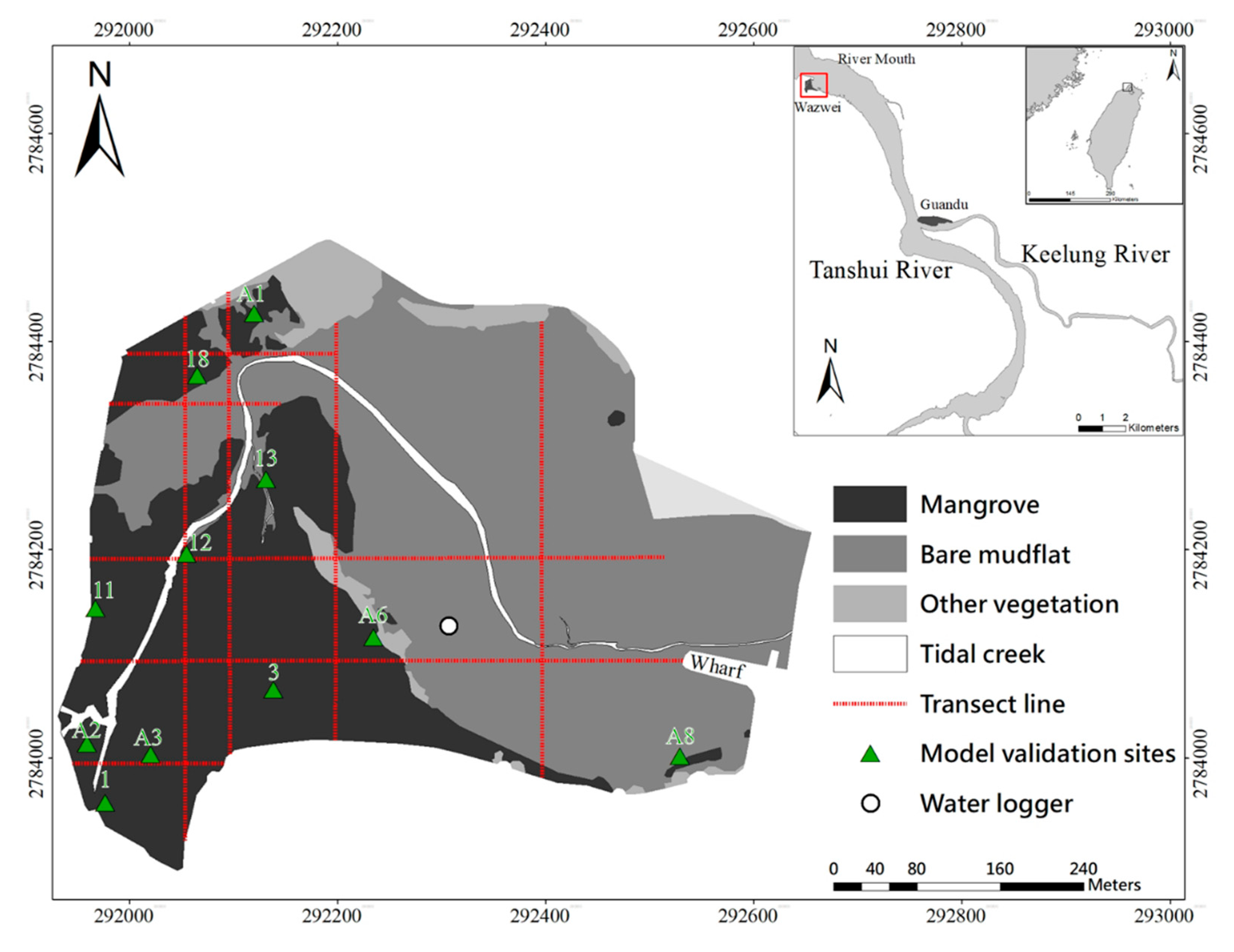
The study areas were located at the Wazwei and Guandu mangrove wetlands in the Tanshui River and Keelung River in northern Taiwan (Figure 1). The M2 tide (lunar semi-diurnal) is the primary tidal constituent in this area, with a mean tidal range of 2.17 m, up to 3 m at the spring tides [17]. The annual mean salinities are 29 ppt and 12 ppt in the Wazwei and Guandu wetlands, respectively [9]. These two mangrove forests constitute the largest population of Kandelia obovata in the Northern Hemisphere [21].
The Wazwei wetland (WZ) was used to develop the SI models on IF and SC factors for K. obovata. The Guandu wetland (GD) acted as the baseline reference site and was adopted to establish a comprehensive HSI model by incorporating the SA factor. The landscape structure of the mangrove wetlands consists of mangrove areas (MT), bare mudflat (BM), and tidal creek (TC). Various bathymetry and inundation features can be found in these three different landscape patches. A comprehensive field investigation of the WZ was conducted (Figure 1). The topography and substrate grain size along the transect lines were measured in 2013 and 2015. The mangrove biomass was investigated from 2010 to 2015, and this investigation included measurements of the mangrove tree heights (H), diameters at breast height (DBH), and tree density.
Twenty-seven sample sites were located in both mangrove and non-mangrove areas for the first model validation (Table 1). Eleven stations marked with green triangles in Figure 1 represent mangrove areas, leaving sixteen stations shared between BM and TC. At the BM stations, there might have been a few seedlings without any adults. To verify the applicability of the model, the GD was adopted for additional model validation. The GD is located at the confluence of the Tanshui River and Keelung River, and the distance from WZ is approximately 10 km. The mangrove species in this area is the same as in WZ, i.e., K. obovata. Thus, this area was identified as an appropriate study area for second model validation.
2.2. Biological Investigations
2.2.1. Mangrove Structure Parameters
A 4 m × 4 m quadrat was used in the field investigation to estimate the mangrove density at specific monitoring sites, where the numbers of trees in the frame were recorded. The numbers of adult K. obovata individuals with tree heights taller than 1.3 m and seedlings were recorded separately. Seedlings are defined here as K. obovata individuals with aboveground heights of less than 1.3 m. The H, DBH, and biomass per unit area of all the trees were measured. In the present investigation, the tree height was measured using a leveling rod. The measured H and DBH values were used as the inputs for the allometric equation derived for K. obovata, which was used to estimate the mangrove biomass. The allometric equation for the aboveground biomass adopted in the present study is from the equation proposed by Khan et al. [22]. This form was originally designed to better estimate the aboveground biomass of mangroves observed in the Guandu wetland in northern Taiwan [23]. The belowground biomass was estimated by the allometric equation proposed by Hoque et al. [24].
2.2.2. Statistical Analysis
A one-way ANOVA model was applied to test whether the H and DBH of mangrove trees differed across measurement times and locations. Before the analysis, these values were examined by the rule given by Clarke and Warwick [25] to ensure they conformed to the normality and homogeneity of variance assumptions. When significant differences were detected in the model, Tukey’s post hoc tests were used to determine the individual mean differences (α = 0.05).
2.3. Environmental Investigations
2.3.1. Substrate Grain Size
A PVC (polyvinyl chloride) pipe with a diameter of 2.6 cm was adopted to collect surface soil samples at depths from 2–3 cm. The samples were then reserved at low temperatures and carried back to the laboratory. The substrate samples were then placed into a Wentworth-series sieve (with a mesh size ranging from 1.0 cm to 62 m) for wet screening. For the silt/clay content (grain size of 62 m), the quantitative pipette method refined by Hsieh and Chang [26] was adopted for analysis. The median grain size was used to represent the particle size of the wetland soil. The calculation of the median grain size and soil sorting coefficient (SC) are given in Equations (1) and (2). The median grain size was used to determine the average conditions of the substrate grain size, while the SC can be utilized to recognize the variation between grain sizes.
where denotes the sieve opening.
2.3.2. Topography
Various measuring technologies were applied to field measurements to acquire the comprehensive elevations of MT, BM, and TC. The elevation of the BM and the TC areas was investigated by using a TOPCON Total Station (GTS226). The elevation of the adjacent cross-section developed by the Tenth River Management Office, Water Resources Agency, Ministry of Economic Affairs, Taiwan, was used as the benchmark reference. The benchmark elevation and water level records were obtained from the Taiwanese fundamental benchmark of Keelung. This fundamental benchmark was determined by the mean sea level and has been adopted as the zero orthometric height of Taiwan. The orthometric height is the height above sea level for practical purposes.
The traditional surveying technologies mentioned above, however, cannot be applied to the MT areas due to the shielding effect of the mangrove forests with their dense foliage and canopy. A communicating vessel system (CVS) was established and presented in this study to overcome this difficulty (Appendix A Figure A1). The CVS was a system of connected tubes filled with water and subjected to the same atmospheric pressure. Our CVS consisted of two transparent acrylic tubes, one connecting hose, and two valves. The connecting hose was covered with water. The water could flow between the hose and the transparent acrylic tubes as the wetland elevation changed. The water in the transparent acrylic tubes remained a free water surface. The valves between the transparent acrylic tubes and the connecting hose controlled the movement of water.
The water depths determined by the CVS were used to measure the elevations across the wetland along the transect lines. At the start of the measurement, the two transparent acrylic tubes were placed on different locations and were kept upright. Then, we opened the valve and recorded the water depths and the straight-line distance of the transparent acrylic tubes when the water levels remained stable. The difference between the two water depths was the elevation difference between the two measurement points. The wetland slope could also be obtained by dividing the water depth difference by the distance. This variation in elevation is calculated by Equation (3).
where ΔH represents the variation in elevation between the two measurement points, H1 and H2, which are the water depths recorded by the CVS.
ΔH = | H1 − H2|
2.3.3. Inundation Frequency
The tidal regime of the Tanshui River is semidiurnal with mixed tides. A HOBO water level logger (model U20-001-01) was installed in a non-mangrove location to monitor the water level every 30 min during all seasons from 2013 to 2015. A PVC pipe was installed to serve as the fixture to attach the water logger. The PVC pipe was 2 m in length and 2 inches in diameter, and holes were drilled along the lateral side to allow water to flow in and out. The water stage records of the Rivermouth gauge station were used for validating the recoded data of the water logger. The Tenth River Management Office constructed the gauge station, and it is located near the study area. The Weibull method was employed to analyze the inundation frequency associated with the different water levels [27]. The inundation frequency was calculated according to Equation (4).
where m denotes the water stage records of m in descending order, and N denotes the total number of data points.
IF = [m/(N + 1)] × 100%
2.4. Mangrove Habitat Suitability Model
Analysis of the species–environment relationship has always been a central issue in ecology [28]. The widely used preference function method for habitat modeling requires quantitative descriptions of the environmental habitat characteristics and quality of life of the species based on the HSI. The HSI can be represented as a function of the univariate habitat suitability curves (HSCs), which explain the degree of preference displayed by organisms for various abiotic variables [14]. First, the available range of the environmental factors was divided into discrete intervals, then, the mangrove biomass falling into each interval was counted, and, finally, the result was plotted as a bar graph.
The discrete HSI values were calculated based on the mangrove biomass within each interval divided by the total mangrove biomass and were normalized to vary between 0 and 1. Two key environmental factors for K. obovata trees were considered, the IF and SC. The HSCs of the two parameters were developed based on sampling data from the Wazwei wetland and show the histograms of the frequencies of K. obovata for different classes of each variable. Piecewise linear functions were employed to establish the habitat models of the individual environmental factors and the combined factors.
These steps have paved the way for the present study to determine the factors affecting the HSI for K. obovata in the Wazwei wetland. An integrated HSI model can be established by combining each single SI model. The minimum function suggested by Hsu et al. [15] was adopted to integrate the SIIF and SISC models, as shown in Equation (5). The method of minimum function indicated equal weight on each single SI model. In addition, Yang et al. [9] presented the variant inundation tolerance of the K. obovata along the Tanshui River for different annual mean salinities. The binomial distribution was applied for modifying the original SIIF along with the relationship of annual mean salinity and inundation frequency, as shown in Equations (6) and (7).
where SA represents the annual mean salinity and IFS,HE and IFS,LE represent the inundation frequencies of the highest and the lowest elevations, respectively, at that specific salinity level.
For the model validation purpose, the simulated SI values were compared with the measured SI values using the Nash–Sutcliffe efficiency coefficient (NSE), as shown in Equation (8), which could be substituted by the root-mean-square error (RMSE), as shown in Equation (9). The NSE values were used to determine the model performance by comparing the results between the model simulations and the field measurements. Following the suggestions of Ritter and Muñoz-Carpena [29], NSE0.90 is classified as a very good simulation, whereas NSE values ranging from 0.80 to 0.90 indicate a good simulation, and values ranging from 0.65 to 0.80 indicate an acceptable simulation.
where is the number of samples; and represent the samples (of size N) containing the observations and the model estimates, respectively; is the mean of the observed values; RMSE is the root-mean-square error; and SD is the standard deviation of the observations.
In addition to comparing the SI scores directly, the present work set a brief criterion to transfer the SI scores to landscape identification. The stations with SI scores less than 0.1, as predicted by the models, were identified as non-mangrove areas from an aerial image. SI values less than 0.1 are transferred to zero, whereas those equal or greater than 0.1 are assigned to 1.0. The transferred values of 0 denote landscape without mangrove tree cover, while the values of 1 represent landscape with visible mangroves.
3. Results
3.1. Biological Investigations
The H and DBH (mean ± SD) of mangrove trees were 5.23 ± 1.92 m and 8.10 ± 3.87 cm, respectively, as illustrated in Figure 2a,b. The tree density and aboveground biomass per unit area were 12,432 ± 13,145 stand ha−1 and 128,406 ± 101,133 kg DW ha−1, as shown in Figure 2c,d. The tree densities measured in 2013 and 2015 were significantly higher than those measured in 2010 and 2011. However, the H and DBH were not significantly different among the three measurement years of 2011, 2013, and 2015 but were all higher than those in 2010. Similar situations in 2013 and 2015 indicate that the mangrove data that were investigated during 2013 and 2015 could be used to develop the model. During the investigation, we found that mangroves withered and died in certain areas. These dead or fallen mangroves were not included in the calculation, which may lead to some opposite results for the dynamic mangrove structure.
Kandelia obovata at stations 1, 3, 11–13, 18, A2, A3, and A6 were found to have higher crown canopies ranging from 4.1 to 9.1 m, compared with the lower canopies ranging from 1.8 to 3.3 m at stations A1 and A8. The maximum average tree height, 8.1 m, was observed at station A2, whereas the maximum average DBH, 12.93 cm, was measured at station A3. The K. obovata in the areas around these two stations were adults and were distributed mainly on the southwestern side of Wazwei. Due to their competitive advantage, few other plant species (e.g., macroalgae and seaweed) can grow near the adults of K. obovata. Juvenile K. obovata were mainly distributed in the areas around stations A1 and A8, where the crown canopy was lower than in other areas. The average heights at stations A1 and A8 were only 2.1 and 3.1 m, respectively, but the density (including adults and seedlings) was the highest in the whole area.
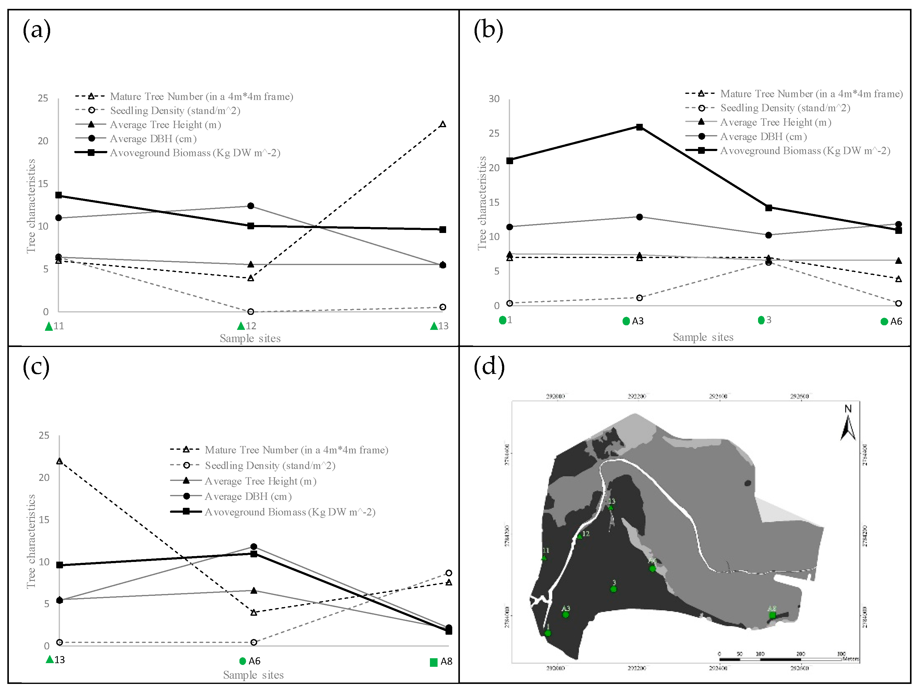
Three virtual routes abstracted from the measurements were adopted to obtain the spatial variation in 2015, as shown in Figure 3. Route (1) consisted of stations 11, 12, and 13, while Route (2) comprised stations 1, A3, 3 and A6, and Route (3) comprised stations 13, A6, and A8. Route (3) can be considered the boundary between the mangrove forest and bare mudflats. The results revealed that the mangrove biomass close to the tidal creek decreased in the direction of expansion. However, the biomass obtained at station 1 was not the maximum value of the corresponding transect line. This result was attributed to the high elevation, which is unfavorable for the growth of mangroves.
3.2. Environmental Investigations
The elevation measurements along the transect lines ranged from 0.6 m to 2.16 m. The terrain under the mangrove trees revealed a higher trend in the southwest area and gradually decreased to the northeast. The eastern mangrove area near the bare mudflats revealed an enormous topography variation resulting from a sand dune that was created as a result of wind effects in winter. The tidal creek had the lowest elevation, while the elevations of the mudflat and sandflat areas were between those of the tidal creek area and mangrove area.
The water level record was collected and revealed that the high tide level ranged from 0.45 to 2.21 m from October 2013 to November 2015. The mean high water level tide (MHWL) was recorded at 1.40 m above sea level, and the mean low water level (MLWL) was recorded at −0.85 m. In this duration, the maximum high tide level occurred on 6 October 2013, which was caused by Typhoon Fitow and the spring tide and reached 2.21 m. The second maximum high tide level occurred in late September of 2015 and was caused by Typhoon Dujuan, reaching 1.96 m. The third maximum record was caused by Typhoon Vongfong and reached approximately 1.91 m on 12 October 2014. Typhoons have a significant impact on the high tide levels of the Wazwei wetland. The long-term water level record acquires the exceedance probability curve. The inundation time and frequency were available through calculations that combined the water level records and topographic measurement results.
3.3. Piecewise Linear Function Model
The SI piecewise linear functions corresponding to the inundation frequency and sorting coefficient are given in Figure 4a and Figure 5a. The regions with low SI values, such as the tidal creek and bare mudflat areas, are colored blue in the SI maps. For the center region of the mangrove forests with high SI values, the color green is used, as shown in Figure 4b and Figure 5b. The corresponding SIIF and SISC values of the location with the highest aboveground biomass of K. obovata per unit area were set as the most suitable with a value of 1.0. The surface elevation in the Wazwei mangrove forest ranged from 0.32 to 1.40 m, while the most suitable condition was found to be 1.05 m. From the water level record, the inundation frequency was between 2.79% and 41.49%, and the most suitable situation was suggested to be 12.76%. The best suitability was observed at the location with a soil grain size of 0.087 cm, with a range from 0.015 to 0.125 cm. For the substrate SC, an interval between 1.93 and 2.69 covered all the values obtained in the study area, while 2.31 was indicated to be the most suitable condition for K. obovata. Two SI models, developed by using piecewise linear functions, are shown in Equations (10) and (11).
The monitoring station corresponding to the high suitable SIIF was A3, whereas the corresponding SIIF values of stations 13 and A8 showed low suitability. The in-situ conditions at station A3 were better than those at stations 13 and A8. This result coincides with the calculation results of the present SI model. For SISC, high suitable conditions were observed at station 1, while low values were obtained at stations 3 and 12. The comparison of SIIF and SISC revealed that stations 1 and A3 were located near each other. Both stations suggested the best suitability indices, which indicates that this region may represent the best-growing conditions for K. obovata in Wazwei.
The topography and mangrove growth conditions demonstrated few changes in 2013 and 2015. We noted that the corresponding SIIF value with IF in the interval between 12.76% and 14.72% equaled 1.0. Compared with the field data, the SIIF map can represent the growth situation of mangroves. The surface elevation near Guanhai breakwater falls within a suitable range for mangroves as well. However, human activities led to the reduced growth conditions of mangroves. The comparison of these two models shows that the area with high SI values increased while the low-value area experienced little variation in the 2015 SI models. This result might represent a higher tolerance to the inundation of K. obovata.
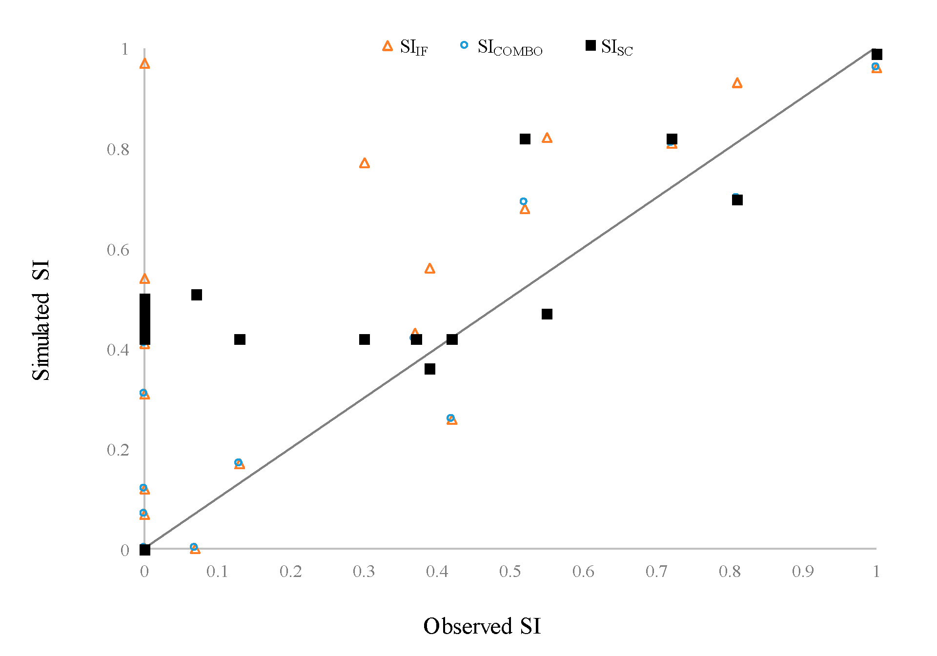
The simulated and observed results, and the corresponding NSE coefficients are illustrated in Table 1 and Appendix A Table A1. The simulation accuracies of the integrated model SICOMBO, the single model SIIF, and SISC compared with field measurements were 89.6%, 85.0% and 77.6% (Table 1), while those simulations compared with the landscape identification were 81.5%, 81.5%, and 59.3% (Appendix A Table A1).
4. Discussion
4.1. Model Accuracy and its Prediction Ability for Potential Distribution
The mangroves in the Wazwei wetland mainly grow from south to north, whereas the mangroves in the vicinity of the Fengfan wharf degrade from northeast to southwest. Most mangroves in the southern area were the oldest ones, indicating that all the mangroves are still able to grow each year and represent a healthy condition. The integrated HSI model, SICOMBO, which considered both SIIF and SISC, could accurately capture the present mangrove biomass distribution (Table 1). The performance of the SIIF model was higher than that of SISC model (Figure 6).
The results identified the reliability of the current model. The residual error may be attributed to human activities and competition with other vegetation. For instance, the surface elevation was within the interval of 1.01 and 1.54 m in the vicinity of the Guanhai wharf. The SIIF model indicated that appropriate environmental conditions for the growth of mangrove trees may exist in the region around Guanhai. However, few mangrove trees grow in that region. The vegetation in this area mainly consists of reeds and Clerodendrum inerme rather than mangroves and their propagules.
The Kandelia obovata in the Wazwei wetland was observed to grow and expand from the southwestern part to the northeastern area. This pattern indicates that those areas with relatively high SI scores; however, few mangrove trees may be a suitable habitat for K. obovata. Nevertheless, the K. obovata community has not yet expanded to this area. In addition, mangroves adjacent to the wooden walkway were found to be influenced by anthropogenic engineering. The growth of K. obovata in this area is not as ideal as the measurements might indicate. On the other hand, there was a small variation between the biomass of stations 13 and A6 on Route (3), as shown in Figure 3. The mangroves at station A8 were juvenile trees, which represented the seedling expansion area.
In addition, the investigation of the soil grain size revealed that the substrate features in the study area varied significantly at the spatial but not at the temporal scale. The mangrove forest and foreshore areas were found to have high water and clay/silt contents. A high proportion of silt and clay in sediments is associated with high organic matter (a proxy of nutrients) and retained water content [30]. Such characteristics are indicative of muddy habitats and feeble currents, which allow organic-matter-laden food particles to rain down from the water column, subsequently favoring deposit-feeding [31,32]. The mangrove habitat is located at relatively high elevations and has a mud substrate and slow water flow, thus suggesting that this habitat is favorable for deposit feeders.
From the first model validation results mentioned above, the SIIF model was more reliable in predictions than the SISC model and approached the ability of the integrated model SICOMBO. The present study utilized the Wazwei SIIF model and the data of IF at Guandu to develop the Guandu SIIF map. We compared the results with the current mangrove conditions for the second validation. Most of the results we found coincided with the current mangrove conditions, except for the area with red cross dots, as shown in Figure 7b.
The lack of sufficient measurement points in the Guandu wetland was deduced to be primarily responsible for this variation, which led to significant deviation when conducting the topography interpolation. Both the inundation time and water salinity level are critical environmental factors for mangroves [17,19,33]. Yang et al. [9] expressed that mangrove inundation tolerance is inversely dependent on the salinity concentration. They also found that the inundations of K. obovata in the Tanshui River were different due to variations in the water salinity and that they obeyed binominal equations, as shown in Equations (6) and (7). This study adopted the suggestion of Yang et al. [9] to revise the model, as illustrated in Figure 7a. The revalidation results are shown in Figure 7c, which revealed more rational prediction results. The results imply that the SIIF model might be practical for more broad applications in other places by incorporating the effects of water salinity on IF.
The primary sources of the modeling errors are summarized as follows, and can be used to direct the advance and improvement of the models in the future: (1) anthropogenic engineering and human activities; (2) other vegetation competition; (3) the systematic error of the bathymetric and terrain survey; and (4) the bias forecasts of the established piecewise linear functions. The findings of the study could be employed to revise the inundation frequency of our model and might increase the accuracy of the model prediction.
Despite other affecting factors, further investigations with a more extended period should be considered in future works. The environmental factors of the current model do not include the temperature, which is also considered a critical factor at the regional scale [34]. This is because this study was focused on the Tanshui River in northern Taiwan. The cold-resistant mangrove forests of K. obovata are the mono-species in the Tanshui River [21]. The temperature difference between the two wetlands is not distinct. If future research considers a broader area and includes other mangrove species, such as Avicennia marina (Forsk.) Vierh. and Rhizophora mucronata Lam., it may be necessary to account for variant temperatures in updating the model. Multivariate analyses might also be taken into account at different mangrove wetlands, e.g., a PCO (principal coordinates analysis) and PCA (principal component analysis) testing site specific biomass against environmental factors.
4.2. Sea-Level Rise Responses and Its Management Implications
The past several decades have experienced climate change and the resulting effects of sea-level rise [35,36,37,38]. Sea-level rises increase both inundation and water salinity levels, which are vital environmental factors for mangroves [39,40]. It is widely acknowledged that such sea-level rises may have a significant impact on the coastal and estuarine ecosystems, including mangrove communities [7,8,19]. Mangrove vegetation may take the tree structure, normally growing above the mean sea level in the intertidal zone of marine coastal environments or estuarine margins [41]. Gilman et al. [8] indicated that most mangrove sediment surface elevations are not keeping pace with the rising sea level.
Although Lovelock et al. [7] suggested the potential capacity of mangroves to keep pace with the sea-level rise and avoid inundation through vertical accretion of sediments, they indicated that sediment delivery in the Indo-Pacific region is declining due to anthropogenic activities, such as the damming of rivers. Shih and Yu [42] found similar impacts where the Shihmen Reservoir stopped most of the watershed sediment upstream of the Tanshui River. Ellison [43] indicated that mangrove forests were able to tolerate sea-level rises of up to 9 cm/100 years. A mangrove forest in Hunger Bay showed a peat accumulation rate of 8.5 to 10.6 cm/100 years over the last 2000 years [44]. Tidal gauge records show that the sea level in northern Taiwan increased at a rate of 24.2 cm/100 years [44], which is higher than the increases mentioned above.
A rising sea level thus has a significant impact on mangroves when they experience a net lowering in sediment elevation, and there is a limited area for landward migration. The inundation frequency has been suggested to be one of the most affecting factors according to previous investigations and the present work. This study considers the sea-level rise effect on mangroves using the established SIIF model by ignoring the sediment deposition of the mangrove wetland. Figure 8 shows the predicted SIIF distribution map considering the rate of sea-level rise of 0.242 cm/year. It is apparent from this SI map that the area suitable for mangrove habitat and growth is predicted to decrease dramatically.
Additionally, the mangrove community in Wazwei was not able to expand landward due to blocking from roads and levees, which is consistent with the conclusions by Yang et al. [9] and Lovelock et al. [7]. This boundary limits the expansion of mangroves to higher-altitude areas as the sea level increases. The predictions can be used to understand the consequences of mangrove habitats after considering the effects of sea-level rise, especially on the inundation time and frequency. The coverage area of mangroves would decrease, while the mudflat would expand its area into the original mangrove area. The forecast of Lovelock et al. [7] suggested that mangrove forests at sites in the Indo-Pacific region, with a low tidal range and low sediment supply, could be submerged as early as 2070. Compared with their results, our present study indicates a relatively low velocity of damage to the mangrove system due to the lagoon geomorphology of the study area, providing a more suitable area for mangrove shifting and habitation.
Mangrove forests were previously recorded in the current bare mudflats. It is deduced that mangrove forests may return to the region in the future according to our investigation. Ximenes et al. [16] suggested that planning restoration of mangroves using spatial analysis tools may contribute to carbon storage projects, because better-developed forest structure provides greater carbon sequestration potential. Although the persistence of mangrove forests within the intertidal zone is influenced by regional sea-level rise and coastal geomorphology, vegetation also affects the soil structure and surface elevation changes, and changes in the location of the mangrove soil surface in the vertical plane [18]. Cheong et al. [45] illustrated that mangroves are not passive to changes affecting them; instead, they maintain a strong ability to modify their environment, to naturally promote habitat persistence, and to serve as engineers for coastal adaptation.
Ye et al. [17] concluded that the mangrove K. obovata would shift from downstream to upstream, where the fresher river water can ameliorate the effects of increased salinities that accompany deeper tidal flooding. Gilman et al. [8] suggested that more research is needed on the assessment methods and standard indicators of change in response to the effects from climate change, while regional monitoring networks are required to observe these responses to enable educated adaptation.
Shih et al. [18] found that the radius/width ratio of a meandering river of less than 3 would lead to vast mudflats, which provide an ideal environment for the growth of mangroves due to their secondary flow. They also suggested that the effect of secondary flow can facilitate mangrove restoration through the creation of bare mudflats. Yang et al. [9] indicated that approximately 63% and 35% of the K. obovata forests on the Zhuwei wetland and the Guandu wetland would vanish by 2100, because levees would limit landward migration. The difference in mangrove loss rates is due to the different local topography.
Cheng and Shih [46] suggested that dike removal would provide a more massive floodplain, which would contain more floodwater to prevent inundation disasters and provide more habitats for mangrove restoration. Twilley [47] suggested that flooded areas adapted to stressful environments for the restoration of mangroves are relatively susceptible. Tradeoffs in urban floodplains in terms of multiple demands for flood control, ecological conservation, carbon stocks, and landscape recreation must be considered and addressed [24,48]. Furthermore, the establishment of a long-term monitoring program is suggested for fixed-station investigations by using SET (surface elevation table). Transect-line surveys, as used in this type of investigation, may be necessary to determine the geomorphic dynamics and mangrove coverage changes and identify the landscape responses of the mangrove wetlands.
5. Conclusions
This study established habitat models for Kandelia obovata mangrove trees through a well-designed survey of the biotic and abiotic factors in the Tanshui River in northern Taiwan. The biological and environmental data showed spatial differences and temporal dynamics. They were both influenced by the watershed flow conditions and sediment inputs. The mangrove tree density, height, and diameter at breast height were not significantly different during the study period, as suggested by the data used to develop the model. We employed piecewise linear functions to establish the habitat models. The inundation frequency had a much higher ability to interpret the variation in the mangrove biomass per unit area than the sorting coefficient of the substrate soil.
The model validations in Wazwei showed good simulation results, with approximately 90% accuracy. After incorporating the effects of different annual mean salinity, the revalidation in Guandu revealed a reliable forecast. Additionally, as mentioned above, the present work used a brief criterion to transfer the SI scores to the predicted landscape identification results. The corresponding results could be applied in pragmatic wetland management and may help to predict the potential areas for mangrove restoration efficiently. The modeling results of the impacts of sea-level rise indicate the shift and decline of the mangrove habitat. As levees have blocked the landward fringes of many mangrove habitats, the restoration of floodplains is suggested to be considered for mangrove habitat rehabilitation.
Author Contributions
S.-S.S. developed the conceptualization, methodology, model development and validation, formal analysis, field investigation, writing—original draft preparation, and project administration.
Funding
This research was funded by the Ministry of Science and Technology (MOST 104-2621-M-002 -022 -MY2, MOST 106-2621-M-002 -004 -MY3) and the New Taipei City Government, Taiwan for funding support.
Acknowledgments
S.C. Huang helped with the substrate investigations and G.W. Hwang commented on the HSI model development. C.E. Hsu helped with the data preparation for writing the draft manuscript. The constructive suggestions from two anonymous reviewers were incorporated into the paper.
Conflicts of Interest
The author declares no conflict of interest.
Appendix A

Table A1.
Comparison of the SI predictions from the SI models and the landscape identification from an aerial photo in Wazwei. The values 0 and 1 represent mangrove areas and non-mangrove areas, respectively. The NSE was used to evaluate the performance of the SI models.
Table A1.
Comparison of the SI predictions from the SI models and the landscape identification from an aerial photo in Wazwei. The values 0 and 1 represent mangrove areas and non-mangrove areas, respectively. The NSE was used to evaluate the performance of the SI models.
| Station | Landscape | SIIF | SISC | SICOMBO |
|---|---|---|---|---|
| 1 * | 1 | 1 | 1 | 1 |
| 3 * | 1 | 1 | 1 | 1 |
| 5 | 0 | 0 | 1 | 0 |
| 7 ** | 0 | 1 | 1 | 1 |
| 8 | 0 | 0 | 0 | 0 |
| 9 | 0 | 0 | 0 | 0 |
| 11 * | 1 | 1 | 1 | 1 |
| 12 * | 1 | 1 | 1 | 1 |
| 13 * | 1 | 1 | 1 | 1 |
| 14 ** | 0 | 1 | 1 | 1 |
| 15 ** | 0 | 1 | 1 | 1 |
| 16 ** | 0 | 1 | 1 | 1 |
| 17 | 0 | 0 | 0 | 0 |
| 18 * | 1 | 1 | 1 | 1 |
| 20 | 0 | 0 | 0 | 0 |
| 25 | 0 | 0 | 1 | 0 |
| 26 | 0 | 0 | 0 | 0 |
| 27 | 0 | 0 | 0 | 0 |
| 28 | 0 | 0 | 1 | 0 |
| 29 | 0 | 0 | 1 | 0 |
| 30 | 0 | 0 | 1 | 0 |
| 31 ** | 0 | 1 | 1 | 1 |
| A1 * | 1 | 1 | 1 | 1 |
| A2 * | 1 | 1 | 1 | 1 |
| A3 * | 1 | 1 | 1 | 1 |
| A6 * | 1 | 1 | 1 | 1 |
| A8 * | 0 | 0 | 1 | 0 |
| NSE (%) | 81.5 | 59.3 | 81.5 | |
* current mangrove area; ** potential mangrove area.
Figure A1.
The schematic plot of the communicating vessel system (CVS) developed by this study for elevation measurement in mangrove areas.
Figure A1.
The schematic plot of the communicating vessel system (CVS) developed by this study for elevation measurement in mangrove areas.

References
- Donato, D.C.; Kauffman, J.B.; Murdiyarso, D.; Kurnianto, S.; Stidham, M.; Kanninen, M. Mangroves among the most carbon-rich forests in the tropics. Nat. Geosci. 2011, 4, 293–297. [Google Scholar] [CrossRef]
- Sheng, Y.P.; Lapetina, A.; Ma, G. The reduction of storm surge by vegetation canopies: Three-dimensional simulations. Geophys. Res. Lett. 2012, 39, L20601. [Google Scholar] [CrossRef] [Green Version]
- Das, S.; Vincent, J.R. Mangroves protected villages and reduced death toll during Indian super cyclone. Proc. Natl. Acad. Sci. USA 2009, 106, 7357–7360. [Google Scholar] [CrossRef] [Green Version]
- Patel, D.M.; Patel, V.; Singh, A.; Katariya, B. Resilience of Tsunami in Coastal Regions of Kachchh by Use of Mangrove Belt and Numerical Modelling. Int. J. Earth Atmos. Sci. 2015, 2, 149–159. [Google Scholar]
- Kathiresan, K.; Rajendran, N. Coastal mangrove forests mitigated tsunami. Estuar. Coast. Shelf Sci. 2005, 65, 601–606. [Google Scholar] [CrossRef]
- Nagelkerken, I.; Blaber, S.; Bouillon, S.; Green, P.; Haywood, M.; Kirton, L.; Meynecke, J.O.; Pawlik, J.; Penrose, H.; Sasekumar, A. The habitat function of mangroves for terrestrial and marine fauna: A review. Aquat. Bot. 2008, 89, 155–185. [Google Scholar] [CrossRef] [Green Version]
- Lovelock, C.E.; Cahoon, D.R.; Friess, D.A.; Guntenspergen, G.R.; Krauss, K.W.; Reef, R.; Rogers, K.; Saunders, M.L.; Sidik, F.; Swales, A. The vulnerability of Indo-Pacific mangrove forests to sea-level rise. Nature 2015, 526, 559–563. [Google Scholar] [CrossRef] [Green Version]
- Gilman, E.L.; Ellison, J.; Duke, N.C.; Field, C. Threats to mangroves from climate change and adaptation options: A review. Aquat. Bot. 2008, 89, 237–250. [Google Scholar] [CrossRef]
- Yang, S.C.; Shih, S.S.; Hwang, G.W.; Adams, J.B.; Lee, H.Y.; Chen, C.P. The salinity gradient influences on the inundation tolerance thresholds of mangrove forests. Ecol. Eng. 2013, 51, 59–65. [Google Scholar] [CrossRef]
- Chen, T.Y.; Hwang, G.W.; Mayfield, A.B.; Chen, C.P.; Lin, H.J. The development of habitat suitability models for fiddler crabs residing in subtropical tidal flats. Ocean Coast. Manag. 2019, 182, 104931. [Google Scholar] [CrossRef]
- U.S. Fish and Wildlife Service. Habitat as a basis for environmental assessment. In Ecological Services Manual; U.S. Fish and Wildlife Service Department of the Interior Washington, D.C.: Washington, DC, USA, 1980; p. 101. [Google Scholar]
- Vincenzi, S.; Caramori, G.; Rossi, R.; De Leo, G.A. A GIS-based habitat suitability model for commercial yield estimation of Tapes philippinarum in a Mediterranean coastal lagoon (Sacca di Goro, Italy). Ecol. Model. 2006, 193, 90–104. [Google Scholar] [CrossRef]
- Shih, S.S.; Lee, H.Y.; Chen, C.C. Model-based evaluations of spur dikes for fish habitat improvement: A case study of endemic species Varicorhinus barbatulus (Cyprinidae) and Hemimyzon formosanum (Homalopteridae) in Lanyang River, Taiwan. Ecol. Eng. 2008, 34, 127–136. [Google Scholar] [CrossRef]
- Boavida, I.; Dias, V.; Ferreira, M.T.; Santos, J.M. Univariate functions versus fuzzy logic: Implications for fish habitat modeling. Ecol. Eng. 2014, 71, 533–538. [Google Scholar] [CrossRef]
- Hsu, C.B.; Hwang, G.W.; Lu, J.F.; Chen, C.P.; Tao, H.H.; Hsieh, H.L. Habitat characteristics of the wintering common teal in the Huajiang wetland, Taiwan. Wetlands 2014, 34, 1207–1218. [Google Scholar] [CrossRef]
- Ximenes, A.C.; Gondim, F.R.; Scott, P.C.; Dahdouh-guebas, F. Spatial analysis framework for mangrove forest restoration: A theoretical case for Itaipu Lagoon, Brazil. Caminhos de Geografia 2016, 17, 32–50. [Google Scholar] [CrossRef]
- Ye, Y.; Gu, Y.; Gao, H.; Lu, C. Combined effects of simulated tidal sea-level rise and salinity on seedlings of a mangrove species, Kandelia candel (L.) Druce. Hydrobiologia 2010, 641, 287–300. [Google Scholar] [CrossRef]
- Shih, S.S.; Yang, S.C.; Lee, H.Y.; Hwang, G.W.; Hsu, Y.M. Development of a salinity-secondary flow-approach model to predict mangrove spreading. Ecol. Eng. 2011, 37, 1174–1183. [Google Scholar] [CrossRef]
- Krauss, K.W.; Lovelock, C.E.; McKee, K.L.; López-Hoffman, L.; Ewe, S.M.; Sousa, W.P. Environmental drivers in mangrove establishment and early development: A review. Aquat. Bot. 2008, 89, 105–127. [Google Scholar] [CrossRef]
- Cohen, J. Statistical Power Analysis for the Behavioral Sciences; Routledge: Abingdon, UK, 2013. [Google Scholar]
- Sheue, C.R.; Liu, H.Y.; Yong, J.W. Kandelia obovata (Rhizophoraceae), a new mangrove species from Eastern Asia. Taxon 2003, 52, 287–294. [Google Scholar] [CrossRef]
- Khan, M.N.I.; Suwa, R.; Hagihara, A. Allometric relationships for estimating the aboveground phytomass and leaf area of mangrove Kandelia candel (L.) Druce trees in the Manko Wetland, Okinawa Island, Japan. Trees 2005, 19, 266–272. [Google Scholar] [CrossRef]
- Shih, S.S.; Hsieh, H.L.; Chen, P.H.; Chen, C.P.; Lin, H.J. Tradeoffs between reducing flood risks and storing carbon stocks in mangroves. Ocean Coast. Manag. 2015, 105, 116–126. [Google Scholar] [CrossRef]
- Hoque, A.; Sharma, S.; Hagihara, A. Above and belowground carbon acquisition of mangrove Kandelia obovata trees in Manko wetland, Okinawa, Japan. Int. J. Environ. 2011, 1, 7–13. [Google Scholar]
- Clarke, K.R.; Gorley, R.; Somerfield, P.J.; Warwick, R. Change in Marine Communities: An Approach to Statistical Analysis and Interpretation; Primer-E Ltd.: Ivybridge, UK, 2014. [Google Scholar]
- Hsieh, H.L.; Chang, K.H. Habitat characteristics and occurrence of the spionid Pseudopolydora sp on the tube-caps of the onuphid Diopatra bilobata (Polychaeta: Spionidae Onuphidae). Bull. Inst. Zool. Acad. Sin. 30 1991, 30, 331–339. [Google Scholar]
- Chow, V.T. Open-Channel Hydraulics; McGraw-Hill: Boston, MA, USA, 1988. [Google Scholar]
- Guisan, A.; Zimmerman, N.E. Predictive habitat distribution models in ecology. J. Ecol. Model. 2000, 135, 147–186. [Google Scholar] [CrossRef]
- Ritter, A.; Muñoz-Carpena, R. Performance evaluation of hydrological models: Statistical significance for reducing subjectivity in goodness-of-fit assessments. J. Hydrol. 2013, 480, 33–45. [Google Scholar] [CrossRef]
- Hossain, M.B.; Marshall, D.J.; Venkatramanan, S. Sediment granulometry and organic matter content in the intertidal zone of the Sungai Brunei estuarine system, northwest coast of Borneo. Carpath. J. Earth Environ. Sci. 2014, 9, 231–239. [Google Scholar]
- Rhoads, D.C. The influence of deposit-feeding organisms on sediment stability and community structure. J. Mar. Res. 1970, 28, 150–178. [Google Scholar]
- Sanders, H.L. Benthic Studies in Buzzards Bay. I. Animal-Sediment Relationships 1. Limnol. Oceanogr. 1958, 3, 245–258. [Google Scholar] [CrossRef] [Green Version]
- Clarke, P.; Allaway, W. The regeneration niche of the grey mangrove (Avicennia marina): Effects of salinity, light and sediment factors on establishment, growth and survival in the field. Oecologia 1993, 93, 548–556. [Google Scholar] [CrossRef]
- Ward, R.D.; Friess, D.A.; Day, R.H.; MacKenzie, R.A. Impacts of climate change on mangrove ecosystems: A region by region overview. Ecosyst. Health Sustain. 2016, 2, e01211. [Google Scholar] [CrossRef] [Green Version]
- Cazenave, A.; Nerem, R.S. Present-day sea level change: Observations and causes. Rev. Geophys. 2004, 42, RG3001. [Google Scholar] [CrossRef]
- Hol gate, S.; Woodworth, P. Evidence for enhanced coastal sea level rise during the 1990s. Geophys. Res. Lett. 2004, 31, L07305. [Google Scholar]
- Thomas, R.; Rignot, E.; Casassa, G.; Kanagaratnam, P.; Acuña, C.; Akins, T.; Brecher, H.; Frederick, E.; Gogineni, P.; Krabill, W. Accelerated sea-level rise from West Antarctica. Science 2004, 306, 255–258. [Google Scholar] [CrossRef] [PubMed] [Green Version]
- Church, J.A.; White, N.J. A 20th century acceleration in global sea-level rise. Geophys. Res. Lett. 2006, 33, L01602. [Google Scholar] [CrossRef]
- Clarke, P.; Myerscough, P. The intertidal distribution of the grey mangrove (Avicennia marina) in southeastern Australia: The effects of physical conditions, interspecific competition, and predation on propagule establishment and survival. Aust. J. Ecol. 1993, 18, 307–315. [Google Scholar] [CrossRef]
- Chen, L.; Wang, W.; Lin, P. Influence of Water Logging Time on the Growth of Kandelia Candel Seedlings. Acta Oceanol. Sin. 2004, 23, 149–158. [Google Scholar]
- Duke, N.C. Australia’s Mangroves; University of Queensland: Brisbane, Australia, 2006; 200p. [Google Scholar]
- Shih, S.S.; Yu, W. Spatial Distribution and Reuse Assessment of Riverbed Sludge of Tanshui River System; Water Resource Agency: Taipei, Taiwan, 2008; (In Chinese).
- Ellison, J. Mangrove Retreat with Rising Sea-level, Bermuda. Estuar. Coast. Shelf Sci. 1993, 37, 75–87. [Google Scholar] [CrossRef]
- Tseng, K.C. A Study on the Sea Level Rise at Taiwanese and Eastern Asia Coasts. Master’s Thesis, National Taiwan Ocean University, Keelung, Taiwan, 2009. [Google Scholar]
- Cheong, S.M.; Silliman, B.; Wong, P.P.; Van Wesenbeeck, B.; Kim, C.K.; Guannel, G. Coastal adaptation with ecological engineering. Nat. Clim. Chang. 2013, 3, 787–791. [Google Scholar] [CrossRef]
- Cheng, T.Y.; Shih, S.S. A model for geomorphological changes of tidal creeks and mudflat. In Proceedings of the 16th Annual Meeting of AOGS, Singapore, 28 July–2 August 2019. [Google Scholar]
- Twilley, R.R. Mangrove wetlands. In Southern Forested Wetlands: Ecology and Management; Messina, M.G., Conner, W.H., Eds.; CRC Press: Boca Raton, FL, USA, 1998; pp. 445–473. [Google Scholar]
- Shih, S.S.; Kuo, P.H.; Lai, J.S. A nonstructural flood prevention measure for mitigating urban inundation impacts along with river flooding effects. J. Environ. Manag. 2019, 251, 109553. [Google Scholar] [CrossRef]
Figure 1.
The study area in the Wazwei wetland, northern Taiwan and the distribution of sampling stations. Nine transects were deployed for the measurement of topography, substrate grain sizes, and mangrove structure parameters. Green triangles represent the mangrove sample sites for the model validations, while the circle represents the water logger site for investigating the water level.

Figure 2.
The biological dynamics of Kandelia obovata mangroves from 2010 to 2015: (a) tree height, (b) diameter at breast height, (c) tree density, and (d) aboveground biomass per unit area.
Figure 2.
The biological dynamics of Kandelia obovata mangroves from 2010 to 2015: (a) tree height, (b) diameter at breast height, (c) tree density, and (d) aboveground biomass per unit area.

Figure 3.
The biological characteristics of K. obovata in mangrove areas along three virtual routes: (a) the spatial variation of sample sites 11, 12, and 13 from southwestern to northeastern, (b) the spatial variation of sample sites 1, A3, 3, and A6 from southwestern to northeastern, (c) the spatial variation of sample sites 13, A6, and A8 from northwestern to southeastern, and (d) the locations of the mangrove sampling sites.

Figure 4.
Development of the SIIF model and corresponding spatial variation of the SIIF values in Wazwei. (a) Piecewise linear functions of the developed suitability index (SI) inundation frequency (IF) (SIIF) model; (b) contour map of the suitability value of inundation frequency-SIIF. The high value represents the most suitable areas for mangrove growth, while zero indicates unsuitable sites for mangroves.

Figure 5.
Development of the SISC model and corresponding spatial variation of the SISC values in Wazwei. (a) Piecewise linear functions of the developed SI soil sorting coefficient (SC) (SISC) model; (b) contour map of the suitability value of the sorting coefficient-SISC. The high value represents the most suitable areas for mangrove growth, while zero indicates unsuitable sites for mangroves.

Figure 6.
Comparison of the simulated and observed SI values at mangrove sample sites. SIIF and SISC are single models considering the inundation frequency and soil sorting coefficient, respectively, while SICOMBO represents the combination of the two environmental factors.
Figure 6.
Comparison of the simulated and observed SI values at mangrove sample sites. SIIF and SISC are single models considering the inundation frequency and soil sorting coefficient, respectively, while SICOMBO represents the combination of the two environmental factors.

Figure 7.
Model validation in the Guandu mangrove wetland. (a) Guandu IF modifications from Wazwei in different annual mean salinities by the binominal equations presented by Yang et al. (2013). The blue line indicates the IF ranges of Guandu and Wazwei in 2013 and 2015. The red line indicates the upper and lower limits of the mangrove area, as suggested by Yang et al. (2013). The black dotted line represents the reference lines for the linear interpolation and extrapolation for producing the modified IF in Guandu, (b) an aerial photo of Guandu in 2015 and the HSI map of the original SIIF model prediction. The red dots indicate where model predictions are wrong, (c) the improved HSI map of the modified SIIF model prediction. A high value indicates the mangrove areas, while a low value indicates areas of mudflats and tidal creeks.

Figure 8.
The predicted inundation frequency distribution map for the Wazwei wetland considering a sea-level rise of 24.2 cm in the year 2100. The high value represents the most suitable areas for mangrove growth, while zero indicates unsuitable sites for mangroves.
Figure 8.
The predicted inundation frequency distribution map for the Wazwei wetland considering a sea-level rise of 24.2 cm in the year 2100. The high value represents the most suitable areas for mangrove growth, while zero indicates unsuitable sites for mangroves.

Table 1.
Comparison of the SI values between the SI model results and field measurements in Wazwei. The Nash–Sutcliffe efficiency coefficient (NSE) was used to evaluate the performance of the SI models.
Table 1.
Comparison of the SI values between the SI model results and field measurements in Wazwei. The Nash–Sutcliffe efficiency coefficient (NSE) was used to evaluate the performance of the SI models.
| Station | Measurement | Simulation | ||
|---|---|---|---|---|
| SIIF | SISC | SICOMBO | ||
| 1 * | 0.81 | 0.93 | 0.70 | 0.70 |
| 3 * | 0.55 | 0.82 | 0.47 | 0.47 |
| 5 | 0.00 | 0.00 | 0.42 | 0.00 |
| 7 ** | 0.00 | 0.97 | 0.47 | 0.47 |
| 8 | 0.00 | 0.00 | 0.00 | 0.00 |
| 9 | 0.00 | 0.00 | 0.00 | 0.00 |
| 11 * | 0.52 | 0.68 | 0.82 | 0.69 |
| 12 * | 0.39 | 0.56 | 0.36 | 0.36 |
| 13 * | 0.37 | 0.43 | 0.42 | 0.42 |
| 14 ** | 0.00 | 0.12 | 0.43 | 0.12 |
| 15 ** | 0.00 | 0.41 | 0.44 | 0.41 |
| 16 ** | 0.00 | 0.54 | 0.46 | 0.46 |
| 17 | 0.00 | 0.00 | 0.00 | 0.00 |
| 18 * | 0.30 | 0.77 | 0.42 | 0.42 |
| 20 | 0.00 | 0.00 | 0.00 | 0.00 |
| 25 | 0.00 | 0.00 | 0.48 | 0.00 |
| 26 | 0.00 | 0.00 | 0.00 | 0.00 |
| 27 | 0.00 | 0.00 | 0.00 | 0.00 |
| 28 | 0.00 | 0.07 | 0.50 | 0.07 |
| 29 | 0.00 | 0.00 | 0.45 | 0.00 |
| 30 | 0.00 | 0.00 | 0.42 | 0.00 |
| 31 ** | 0.00 | 0.31 | 0.46 | 0.31 |
| A1 * | 0.13 | 0.17 | 0.42 | 0.17 |
| A2 * | 0.72 | 0.81 | 0.82 | 0.81 |
| A3 * | 1.00 | 0.96 | 0.99 | 0.96 |
| A6 * | 0.42 | 0.26 | 0.42 | 0.26 |
| A8 * | 0.07 | 0.00 | 0.51 | 0.00 |
| NSE (%) | 85.0 | 77.6 | 89.6 | |
* Current mangrove area; ** potential mangrove area.
© 2020 by the author. Licensee MDPI, Basel, Switzerland. This article is an open access article distributed under the terms and conditions of the Creative Commons Attribution (CC BY) license (http://creativecommons.org/licenses/by/4.0/).
Share and Cite
MDPI and ACS Style
Shih, S.-S. Spatial Habitat Suitability Models of Mangroves with Kandelia obovata. Forests 2020, 11, 477. https://doi.org/10.3390/f11040477
AMA Style
Shih S-S. Spatial Habitat Suitability Models of Mangroves with Kandelia obovata. Forests. 2020; 11(4):477. https://doi.org/10.3390/f11040477
Chicago/Turabian StyleShih, Shang-Shu. 2020. "Spatial Habitat Suitability Models of Mangroves with Kandelia obovata" Forests 11, no. 4: 477. https://doi.org/10.3390/f11040477
Note that from the first issue of 2016, this journal uses article numbers instead of page numbers. See further details here.