Abstract
The tropical rainforest is one of the lushest and most important plant communities in Mexico’s tropical regions, yet its potential distribution has not been studied in current and future climate conditions. The aim of this paper was to propose priority areas for conservation based on ecological niche and species distribution modeling of 22 species with the greatest ecological importance at the climax stage. Geographic records were correlated with bioclimatic temperature and precipitation variables using Maxent and Kuenm software for each species. The best Maxent models were chosen based on statistical significance, complexity and predictive power, and current potential distributions were obtained from these models. Future potential distributions were projected with two climate change scenarios: HADGEM2_ES and GFDL_CM3 models and RCP 8.5 W/m2 by 2075–2099. All potential distributions for each scenario were then assembled for further analysis. We found that 14 tropical rainforest species have the potential for distribution in 97.4% of the landscape currently occupied by climax vegetation (0.6% of the country). Both climate change scenarios showed a 3.5% reduction in their potential distribution and possible displacement to higher elevation regions. Areas are proposed for tropical rainforest conservation where suitable bioclimatic conditions are expected to prevail.
1. Introduction
Tropical ecosystems are essential because of the ecosystem services it provides (food, medicines), its biological richness and its relevance in supporting life [1]. Tropical rainforest (TR) are plant communities found in warm humid areas and include tropical rainforest and tropical sub-evergreen forest communities. Their dominant species have a perennial physiognomy, that is, they are trees that are more than 30 m high and do not change their leaves seasonally [2]. It is the richest vegetation in floristic composition and biotypes in Mexico’s tropical areas, but it currently has a limited and fragmented distribution. In addition, much of it is in early successional stages [3]. In the country, TRs in a mature state (old growth or climax) occupy 12,250 km2 (0.6% of the national territory) according to the last official report in 2016 [4]. The rest of its successional stages occupy 1% of the country’s area; the original distribution area is unknown.
There is greater anthropogenic pressure on TRs than on temperate forests and they are subject to greater landscape fragmentation [5]. During the last century in Mexico, at least 90% was cut down and its use was changed to agriculture, livestock or agroforestry purposes marked by low floristic diversity [3]. Landscapes with substantial differences in plant cover [6] or landscapes fragmentated by deforestation can be found in Veracruz or Chiapas southern states [7]. In addition, climate change has recently been added as a relevant challenge for the ecosystem [8,9].
Mexico’s location between two oceans and its complex relief lead to it being particularly impacted by climate change. For the period 2015–2039, annual temperature increases of 1–1.5 °C are estimated for most of the country and up to 2 °C for the northern zone. For precipitation, decreases of 10–20% are projected, as well as variation in its seasonal distribution. El Niño variability on regional scales likely intensifies [10]. Given these circumstances, it is necessary to know how the change in climate will affect the future geographic distribution of TRs in order to promote actions in the short term aimed at their conservation. There is evidence that many terrestrial species have shifted their geographic ranges in response to ongoing climate change [11]. TRs support great associated biological diversity [1], which may be indirectly affected by climate change. To assess the effects of climate change on natural systems such as ecosystems, long-range time horizons are recommended, such as 2075–2099 [12,13]. With the above, possible adverse effects on the level of natural systems are covered, since ignoring long periods could lead to an underestimation of their impact. In addition, a vision at a higher organizational level than the specific one (for example, of plant community or ecosystem) is needed to assess the possible impacts that climate change can have on the potential distribution (PD) of most of their floristic components [14,15]. In this study, the potential distribution area is defined as the land occupied by a species plus invadable distributional area, where the abiotic and biotic conditions are suitable (see Section 2.3 below).
There are several methods for modeling the geographic and potential distribution of species. Some use environmental information as a dependent variable and species records as independent variables. These can be counts, presences and absences, or only presences [16]. The most common method is Ecological Niche Modeling (ENM) and associated Species Distribution Modeling (SDM) [17,18], which have their theoretical bases in the Hutchinson duality [19]. This refers to the environmental conditions where the species lives (ENM) and its corresponding geographic space (SDM) [17,18]. Among the best known techniques and software are BIOCLIM, Generic Algorithm for Rule-Set Prediction (GARP), Generalized Linear Models (GLM), Artificial Neural Network (ANN) and Maximum Entropy (Maxent) [19,20,21,22]. Results obtained with the different techniques may be subtly or dramatically different and may vary due to differences in the performance of different software [21,23]. In the case of Mexico and TR communities, the PD of some species has been previously studied using ENM and SDM with the GARP method [1]. However, higher performance has been obtained with Maxent [22,24], which was selected in this study.
The aims of the work were: (1) to obtain the potential distribution of 22 species that have ecological value and are representative of tropical rainforests under current conditions and future climate change ones, by applying the ENM and SDM techniques through Maxent and Kuenm—they were chosen for their good performance, use and operation [25]; (2) to intersect the areas with the greatest potential distribution in the current and climate change scenarios, in order to identify areas of potential change (increase, decrease, permanence) of the ecosystem; (3) based on the previous objective, to propose areas for conservation of TRs based on climate change and the distribution of their species, also considering current land use and official protection areas. The results contribute to the debate in two ways: by modeling, with cartographic techniques, the potential distribution of an ecosystem based on its species, as other studies have proposed [9,26], and by discussing and providing basic information for decision-makers on environmental legislation and protection. Anticipating the effects of climate change should serve as a tool for proposing areas for conservation based on the richness of potential distributions.
2. Materials and Methods
2.1. Species Selection
The species were selected for their ecological importance according to the old growth or climax stage of the TR (literature review) and also for their structural value. The ecological importance was based on information extracted from the works of Miranda and Hernández [2], Pennington and Sarukhán [1] and Rzedowski [27]. All of them are Mexican biological and plant species references. Afterwards, two structural valuation indices were applied: importance value (IVI) [28] and forest value (FVI) [29]. Both are common in ecological studies [30]. IVI evaluates dominance, density and frequency, while FVI evaluates diameter at breast height, height and crown cover of the species. Information for the indices was obtained from the National Forest and Soil Inventory (NFSI) for the period 2004–2007 [31,32] and from [4], spatially managed in ArcMap (ESRI) (version 10.5). The results allowed the selection of 22 species (Table 1); the ranking of the ecological and forest value of the species is presented in Supplementary Material S1 (SM1).

Table 1.
Species with ecological and forest importance for Mexico’s tropical rainforest.
2.2. Geographic Records and Bioclimatic Variables
The presence data for each species or geographic records (GRs) were obtained from the NFSI [31] and the Global Information Facility [38]. Prior to downloading, GBIF information was filtered by country and geographic coordinates. The information was reviewed to eliminate duplicate data as well as those outside the natural range of the species (urban areas, lakes or oceans). To reduce the sampling bias that often occurs with this type of data (presence only), their spatial autocorrelation was reduced, as recommended by some authors [39], by random filtering or thinning in 5 or 10 km grids. An alternative to using grids is to use the spThin R package [39]. A mesh spacing of 5 km was used when the number of GRs was low (<1500 GR) and 10 km when it was high (>1500 GR). The databases were divided into three spatially unrelated groups with ENMeval, an R package developed by Muscarella et al. [40], to be used in the following modeling phases: training (57 to 69% GR), testing (20 to 32% GR) and final evaluation (10 to 12% GR) of the models. These percentages were varied in order to ensure good representativeness of the group used for the training of the models.
Regarding current bioclimatic variables, the 19 variables developed for BIOCLIM [21] in 1996 and described by O’Donnell and Ignizio [41] were considered. These are biologically significant when combining precipitation and temperature over the course of the year and not only the annual averages [42]. The bioclimatic variables of the current scenario were obtained from WorldClim [43], after which their level of detail was increased according to Gómez et al. [44], who suggest following the delimitation of areas with homogeneous temperature and precipitation called climatic influence areas. Two climate change scenarios were applied: HADGEM2_ES and GFDL_CM3, both for RCP 8.5 scenarios to 2075–2099. The use of these climate change scenarios has been appropriate for climate change studies [9,36] and is recommended since the uncertainty in natural systems is considerable [12]. The General Circulation Models (GCM) were obtained from Fernández et al. [45]. The applied scenarios are considered to represent an increase of up to 4 °C in the average temperature for that period [46], which may be too great for some ecosystems to cope with [11]. The climate change scenarios were also processed using the methodologies of [41,44] to be comparable with current scenarios.
2.3. Niche and Species Distribution Modeling
Area M or the accessible area of the BAM diagram by Soberón and Peterson [47] was considered to limit the PD of the species to the space that they could colonize when the interactions between them are omitted [18,47]. Area M refers to the ecological and geographic space where species have the potential to disperse, either because of their historical or relatively recent condition [18,19]. Thus, six M areas were defined for equal groups of species with differences in their distribution. For the above, the country’s terrestrial ecoregions were taken as a reference [48] as recommended by [49]. It was then fitted according to the geographic distribution reported in the literature as well as that presented by the GRs for each group of species. The bioclimatic variables were spatially cut to fit the M areas.
A pre-selection of variables was made based on Pearson’s correlation coefficient in order to avoid overfitting the models [20] by including variables that are not biologically important [49] and that are redundant in terms of the information they provide. With Maxent, the selection of models free of overfitting is not a problem as it can deal with collinearity between environmental covariates with the regularization choices [49].
Both ENM and SDM were obtained with Maxent (American Museum of Natural History, New York, NY, USA. version 3.4.0) [25] and with the Kuenm R package (The University of Kansas, Lawrence, KS, USA version 1.1.5) [50] in RStudio [26]. The ENM stages consisted of the creation and evaluation of candidate models, and the creation and final evaluation of the best models. The candidate models were created by correlating the pre-selected variables with the GRs and by varying the parameterizations of the Maxent models (regularization parameters and features). The evaluation of the candidate models for the selection of the best model was based on statistical significance with the partial area under the Receiver Operating Characteristic curve (partial ROC) and predictive power (performance) with 5% omission error rates. Complexity was estimated with the Akaike Information Criteria corrected by sample (AICc) according to [51] and implemented in the Kuenm package [50].
The partial ROC criterion was used to verify that the model is not equal to one given by chance by presenting a non-significant p-value [52]. To the extent that the partial ROC tends to 0, there is greater significance in the model. In fact, this statistic is more appropriate than the full area under curve (AUC) for assessing statistical significance [52]; for details of the calculation, see [50]. With the omission rate criterion, the inability of the model (created with training GRs) is obtained to correctly predict the test GRs at a permissible error [53]. The original AIC statistic provides an estimate of the relative information that is lost when varying the models, since it is a measure of compensation between their goodness of fit and their complexity [54]. Thus, complex models are penalized and preference is given to simpler models [55].
The best potential distribution models were created with the training and test GRs as well as the optimal parametrizations using 10 bootstrap replicas with logistic output. The logistic output was interpreted as a level of climatic suitability for the species [9,49]. The best models were evaluated with the final evaluation data with the partial ROC and omission rate criteria using the same package (Kuenm).
2.4. Mapping Potential Distribution and Percent Changes
The binary potential distribution maps of each species were reclassified into non-potential distribution (NPD) and potential distribution (PD) categories. PD was defined with values equal to or greater than 0.3, while NPD refers to values lower than 0.3. Thus, a binary distribution layer was obtained for each species and for each scenario. Using cartographic processes, changes in PD were identified by applying climate change scenarios for each species. The PD in the current scenario was compared to the PD of both future scenarios through the geographic unions of the maps. Additionally, the current PD of each species was compared with the PD obtained in a previous study [1] to contrast the differences shown by the GARP and Maxent methods, as well as by GRs (until 2005 and 2019, respectively).
Plant communities necessarily include ecological communities, since the former provide the necessary conditions for the latter to develop [56,57]. Thus, our idea is that the trends in PD of the main species can indicate the long-term trend of the plant community (tropical rainforest). For this reason, the PDs of all species in each scenario were assembled, grouping them into three potential distribution classes but now with the TR according to the accumulated percentage. Adequate-PD was defined as occurring when a coincidence of 14 to 22 species was found, Possible-PD when there were 8 to 13 species and Non-PD when there were fewer than 7 species. This information was used for the conservation area proposal. This is based on the perspective of the integrated plant community theory, which indicates that where favorable environmental conditions for a plant community are repeated, the species will reappear. This is because the classification is based on similarities [58,59]. Plant communities lack precise borders [2,56], so our hypothesis is based on the idea that the joint presence of species approximates the TR area. Some species require the presence of others in order to coexist, either at the same time or at different times [56]. Regardless of the species, the interactions between species are key in determining the ecological niche of a single species and, therefore, its range [47].
2.5. Proposed Conservation Areas
In the proposal for TR conservation areas, priority was given to areas where, when considering climate change, future PDs are expected to prevail or increase. Nationals, state, and voluntarily-conserved protected natural areas [60,61] as well as land use and vegetation [4] were compared to areas where the greatest similarity in prevalence or increase in future PDs is projected by climate change scenarios.
3. Results
3.1. Geographic Records and Bioclimatic Variables
Some authors point out that the number and quality of GRs directly influence the performance of the models, and consequently, the approximation of the species’ PD [42,49]. In the present study, an adequate number of GRs was used, since after 14 cleaning and thinning the lowest number of GRs obtained for a species was 85, and Maxent performs well with less than 25 GRs [49,62]. We can see that sampling errors in large databases (such as GBIF) are common due to the heterogeneity of the conditions in which the data are obtained [17], which leads to sampling biases [24,49] and, of course, to duplicate records. Sampling biases also occur because certain areas are not intensively sampled or are not even sampled at all. In other cases they are oversampled [17]. The location of the samples is influenced by accessibility and sometimes by weather conditions, causing the probability of the SDM to favor the oversampled areas [49]. When GR thinning is done, this sampling bias is reduced in areas that have been oversampled but the risk of omitting important data is increased (due to lacking information) [62]. For this reason, the thinning procedure was applied to GRs in a random manner to avoid systematic software errors.
The species with the lowest number of GRs after cleaning and thinning was Guatteria anomala (with 85) and the one with the highest number was Bursera simaruba (with 2607). The number of GRs from each source (NFSI and GBIF) was variable for each species. Specific information is presented in Supplementary Material S2 (SM2). Information on bioclimatic variables and their selection, plus details concerning the six M areas used are included in Supplementary Material S3 (SM3). Warm-humid and warm-dry rainforest ecoregions were taken into account for species delimitation. Other ecoregions were considered when species (seven cases) were reported to be more widely distributed.
3.2. Niche Modeling and Species Distribution
For the species, the AUC ratio ranged from 0.730 to 0.952 and was considered acceptable (Supplementary Material SM5—Table S15). The best models of all species were significant (partial ROC = 0) and not very complex (delta AICc < 2). Only for T. amazonia and H. donnell-smithii were omission rates of 5.6 and 10.9%, respectively, obtained; the models of the other species had good predictive power (Error < 5%). In the final evaluation of the optimal models, there was excellent significance (partial ROC = 0) and variable omission rates (0 to 15.4%). The models obtained are better than a model given by chance (partial ROC = 0); their complexity and omission rates were variable. Applying GR thinning and discarding variables with the highest Pearson’s correlation coefficient and less biological importance could be decisive in obtaining intermediate values of AUC (AUC = 0.5 is equivalent to a model given by chance), but a too high AUC (close to 1) is not an indication of a good model; in fact, it may be an indication of overfitting [25,52]. Applying the model used here resulted in models that perform better with new data if the model is good despite not having high AUCs [49,50]. The above is observed in the models obtained, because most did not present high AUCs but performed acceptably with new data (0 to 15.4% omission rates in the final evaluation phase (see Supplementary Material SM4)). The use of a single set of GRs may have been the reason for the highest omission value (15.4% for Vochysia guatemalensis). The training data set may be iterative (variant for one GR training group), for which replicates should be made with each GR group after which the average map obtained [63], which would have certainly improved the results. It has been found that the accuracy of the models is greater when considering species with small geographic ranges and limited environmental tolerance [62], that is, more accurate models are obtained from rare species than from widely distributed ones. Detailed information about the modeling is shown in Supplementary Material (SM4). For nine species, it was found that the variable with the greatest contribution was precipitation of wettest month (BIO13), for four species it was precipitation seasonality (BIO15) and for four other species it was temperature seasonality (BIO4) (Figure 1).
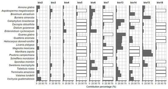
Figure 1.
Contribution of bioclimatic variables to the Maxent models. White bars indicate variable not used. (BIO1 = Annual mean temperature, BIO2 = Mean diurnal range, BIO3 = Isothermality, BIO4 = Maximun temperature of warmest month, BIO6 = Minimun temperature of coldest month, BIO7 = Temperature annual range, BIO8 = Mean temperature of wettest quarter, BIO9 = Mean temperature of driest quarter, BIO10 = Mean temperature of warmest quarter, BIO11 = Mean temperature of coldest quarter, BIO12 = Annual precipitation, BIO13 = Precipitation of wettest month, BIO14 = Precipitation of driest month, BIO15 = Precipitation seasonality, BIO16 = Precipitation of wettest quarter, BIO17 = Precipitation of driest quarter, BIO18 = Precipitation of warmest quarter and BIO19 = Precipitation of coldest quarter).
3.3. Mapping Potential Distribution and Changes
The current PD scenario of the species is shown in Figure 2. Dialium guianense has the smallest PD, while E. cyclocarpum and T. rosea have the broadest. The coincidence of the current PD area of our study with that obtained by Pennington and Sarukhán [1] was relatively low: the PD areas of M. mexicana, G. anomala and S. morototoni in our study differ with respect to the PD of the aforementioned authors by at least 50% of the area and have higher values, while the PD of G. glabra, P. campechiana and C. brasiliense of our study also show a percentage variation but have lower values. More details of the comparison can be found in Supplementary Material (SM5).
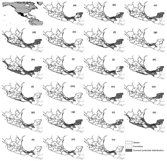
Figure 2.
Current potential distribution of the species. (a) Annona glabra; (b) Aspidosperma megalocarpon; (c) Brosimum alicastrum; (d) Bursera simaruba; (e) Calophyllum brasiliense; (f) Cecropia obtusifolia; (g) Dialium guianense; (h) Enterolobium cyclocarpum; (i) Guarea glabra; (j) Guatteria anomala; (k) Heliocarpus donnell-smithii; (l) Licania platypus; (m) Magnolia mexicana; (n) Manilkara zapota; (o) Pouteria campechiana; (p) Schefflera morototoni; (q) Spondias mombin; (r) Swietenia macrophylla; (s) Tabebuia rosea; (t) Terminalia amazonia; (u) Vatairea lundellii and (v) Vochysia guatemalensis.
At least 14 species show the potential to occupy 97.4% of the territory currently occupied by the climax stage (Figure 3). According to INEGI [4], the climax stage is distributed in 0.6% of the country (12,250 km2). Other potential distribution areas are distributed in land use, mainly agricultural, pasture and different ecological succession of forests as shrub or herbaceous sprouts (Supplementary Material SM5—Table S16).
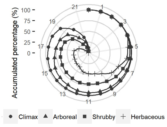
Figure 3.
Accumulated percentage of the potential distribution area of the 22 species within the current Tropical Rainforest area.
Figure 4 shows the potential distribution of the 22 species, both for the assembly of all species (a) and for the three defined classes (b): Adequate-PD (14 to 22 species), Possible-PD (8 to 13 species) and Non-PD (equal or below 7 species). It can be seen that the Tuxtlas-Chimalapas region (southeast and center of the country, in the states of Veracruz, Oaxaca, Tabasco and Chiapas, number 3 and 6) is well represented by the assembly map. This is not the case for the Huastecas region (north of the state of Veracruz and south of the state of San Luis Potosí, number 1), nor for the Huasteca Potosi or Veracruzana region, as they are not represented in the expected class of the greatest representativeness.
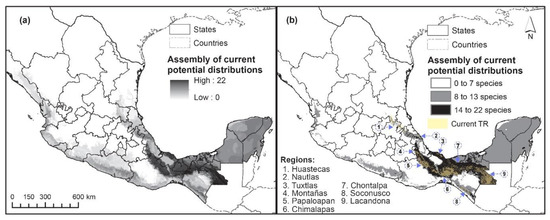
Figure 4.
Current potential distributions for the 22 tropical rainforest species considered in this study. (a) Assembly map; (b) assembly map with three classes.
For the TR adequate-PD class, which represents a coincidence of at least 14 species, an occupation of 85,930 km2 was found, equivalent to 4.45% of the country. According to INEGI [4], current land use is made up of 36% cultivated pasture, 29% at some successional TR stages, 15.5% annual rainfed agriculture, 1.9% water bodies, 1% urban and 17.6% other uses. The most considerable areas of intersection with other plant communities are with cloud forest in its shrub (2%) and old growth stages (1.8%) and with the pine-oak forest arboreal stage (1.65%). For more details, see Supplementary Materials SM5.
Some differences in the PDs in our study with respect to those of Pennington and Sarukhán [1] may be due to the highly different performance by the Maxent and GARP algorithms [23,62]. Some of these differences are: the limit used in the definition of the binary layers (variable: determined by statistics; fixed: 0.3 presence probability), as well as the set of variables and GRs used in the creation of the models [40,42,62,64] and the periods in which it was carried out (2005 and 2019). However, there are coincidences towards the center of PD in most cases, possibly because the algorithms tend to be accentuated in the areas with a higher GR density, meaning that it is possible that the bias was not adequately reduced for all species, or that there are areas remaining to be sampled.
Climate change scenarios. The two climate change scenarios showed similarities in future PD areas (Figure 5) and percent changes (Figure 6). More information and details are presented in Supplementary Material SM5.
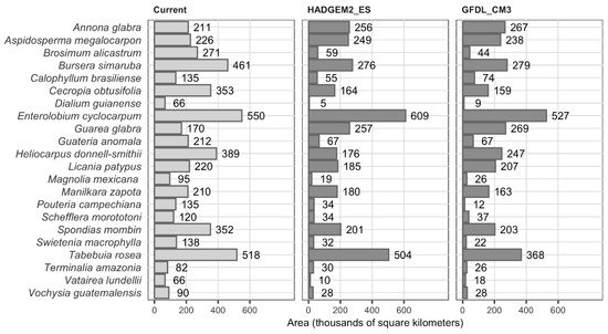
Figure 5.
Potential distribution area in the scenarios considered. The darker gray color indicates the climate change scenarios.
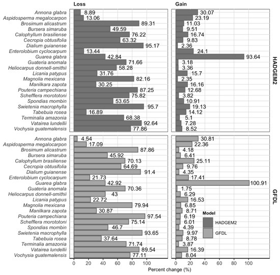
Figure 6.
Changes (percentage) in the potential distribution area of all species considered in the climate change scenarios. (loss refers to the area currently occupied by a given species that will no longer be suitable in the future; gain is for new areas outside the current distribution that will be suitable in the future).
Figure 7 shows the projected changes for climate change assemblies for both scenarios. Additionally, the expected changes by number of matching species are shown (c and d). Considerable decreases in the TR Adequate-PD category are marked in the Tuxtlas-Chimalapas, Soconusco and Southern Tabasco regions, which are larger in these areas than the others (Figure 4). The increase in PD is mostly seen in the higher elevation regions, in the Huastecas and the Nautlas, while greater prevalence is indicated in the Lacandona rainforest region. The GFDL_CM3 model suggests higher humidity in the south of the country, while for the HADGEM2_ES model, they are more restrictive. However, those regions where more than 14 species coincide are considered optimal for conservation (dark green in c and d).
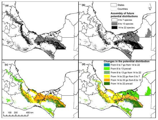
Figure 7.
Assembly map of the projected future potential distribution (a) HADGEM2_ES and (b) GFDL_CM3 climate change scenarios. Potential distribution change by class in (c) HADGEM2_ES and (d) GFDL_CM3 scenarios.
In the HADGEM2_ES scenario, decreases in the TR Adequate-PD category are projected to be 3.5% nationally. A similar situation is observed with the GFDL_CM3 scenario (see Supplementary Material SM5). According to the latter scenario, there are differences in areas of prevalence and loss of PDs, which are presented in Figure 8a. This means that two climate change scenarios find future coincidences in environmental variables that define potential distribution of 22 TR species.
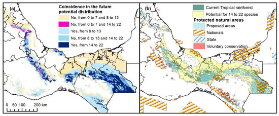
Figure 8.
Proposed areas for Tropical Rainforest conservation in Mexico. (a) Coincidence in the future potential distribution by both climate change scenarios. (b) Proposed areas for conservation based on the coincidence of the future potential distribution of high species number (14 to 22) in both GFDL_CM3 and HADGEM_2 climate change scenarios.
3.4. Proposed Conservation Areas
The conservation of 16,850 km2 is proposed because the PD there is expected to be conserved for at least 14 species according to both climate change scenarios without considering the species emigration (Figure 8b). These are also the places where the best conserved TR relics are located in Mexico [3], that is, the Lacandona rainforest and the regions of greater elevation than the current PD area and where TR actually exists according to official cartography [4].
4. Discussion
4.1. Niche Modeling and Species Distribution
This study considered the species with the highest structural index and those frequently mentioned in the literature. Such species resemble what in conservation biology are known as umbrella species (subset of the surrogate species), and their use in plant communities seems to be promising, since they are frequently used for modeling and protecting animal species. Despite being widely distributed [2,17,65], these species were considered in this study because they are a structural part of the plant community, and it would not be functional without some of these elements [66]. Furthermore, the transitions between successional stages occur gradually [57] and the presence of these species may be a reflection of this condition. Just a few species are used in planning the conservation of larger food webs to ensure that other coexisting species are also conserved. In fact, it is often used [67] in defining the minimum size of the area to be conserved, although this does not guarantee the conservation of rare or human interest species [68]. In this study, Ampelocera hottlei (Standl) Standl and Trophis racemosa (L.) were found to be important as they presented high rates of structural importance as in other TR studies [30].
A high percentage (85%) of the current area with TR fell into the Adequate-TR category. At least 14 species have the potential to occupy almost all of the current TR area (97.4%), which is enough to represent the old growth community and plan its conservation. It is possible to consider more species in further studies (e.g., in the Huasteca region), but the improvement in models and mapping may not be significant. Thus, we consider that our results contribute to TR conservation planning, particularly in old communities as well as in early ones.
The PD of the species is concentrated in the regions with the largest current surface area, that is, in the southern regions, called the Chimalapas and the Lacandona rainforest (see Figure 4b). However, there is a greater level of PD in the regions dedicated to agricultural and livestock use (52%), which coincides with the deforestation pattern experienced by TRs in Mexico during recent decades [2,69]. In regions where TR existed, several grass species were cultivated; however, there were also native species, which maintained the herbaceous successional state due to the continuous use of fire by its inhabitants to accelerate the re-growth of grasses [2]. This prevented the development of later successional stages [57]; this condition still persists [70]. If this alteration ceases, the community could repopulate the surrounding areas. The variants of this plant community are very diverse, as are those of the emerging secondary vegetation [2]; perhaps this is the reason why the current distribution area was not fully covered, which, although it was not this study’s objective, was taken as a guide to measure the degree of certainty of the results.
The areas overlapping with other communities occur with the cloud forest shrub phase (2%) and with its old growth stage (1.8%), as well as with the pine-oak forest arboreal stage (1.6%). The overlaps can help in identifying ecotones, places where there is a combination of plant elements from different communities and which normally have greater floristic diversity [59,71]. The communities and their successional stages have no well-defined boundaries and they happen gradually; moreover, they are the result of their environment and the interactions between their biotic and abiotic elements.
While it is true that obtaining a more refined approximation of a species’ PD requires considering interactions (including exclusionary interactions, not just symbiosis), our results approximate the original distribution because the methodology included: the interactions (biotic component, B); the environmental variables (abiotic component, A) and the M or accessible area (component M). Thus, the BAM diagram [47] was almost completely covered, indicating the conditions necessary for a species to live.
4.2. Projected Changes and Proposed Conservation Areas
The climate change scenarios consistently showed reductions in future PD. In small regions, there is an improvement in climate variables and, consequently, an increase in the conditions for TR growth. Moreover, the pressure and trend observed for species in humid tropical ecosystems is towards fragmentation and reduction. Hence, the scenario worsens for rare or small distribution species [7,72,73]. This pattern was reproduced both in individual species modeling and in the cartographic assembly of the species studied. Reduction in the largest current distribution areas and a possible shift to higher regions are expected. The PD areas in the TR Adequate-PD category (14 to 22 species) of the future scenarios were located in the areas that currently correspond to cloud forest (also in the Lacandona rainforest in the state of Chiapas). When compared to similar studies carried out for cloud forest [9], it is possible to foresee a more accentuated combination of floristic elements between both communities due to the change in their PD. However, in this study, we did not consider integrating the future adaptability of trees, appointed as the ability of forest species to grow successfully under climatic conditions different from those of their natural distributions [74].
In the base scenario and for most of the models, a significant contribution of the extreme values was found in the explanation of the model. Some cases referred to in the literature only refer to the TR from annual averages, that is, an average annual rainfall greater than 2000 mm with up to three or four months with 60 mm, an average annual temperature from 22 to 26 °C but not less than 20 °C and an average monthly temperature above 18 °C with fluctuations from 5 to 7 °C. They also refer to the “tropical rainy” climate that occurs in the TR [1,75]. However, our results indicate that intra-annual attributes are significant, such as the rainfall of the wettest month and its seasonality. We also found that the rainfall of the wettest month explains the PD of at least nine species studied. The above coincides with what Miranda and Hernandez [2] stated about TR distribution: not only is abundant precipitation necessary, but also its availability throughout the year. With increasing global warming and climate change, TR ecosystems may be at risk of abrupt and irreversible changes [11]. It is, therefore, important to have results that show the risk of exchange in conditions suitable for the TR. Many species will be unable to track suitable climates. As appointed by the Intergovernmental Panel on Climate Change -IPCC [11], the maximum speed at which a tree species can move across landscapes is below 20 km per decade.
Ecological niche studies are important to understanding the ecology of TR. Potential distribution shows potential to be used as complement research in conservation studies. The choice of proposed conservation areas took into account the long term since it is the most suitable for modeling changes in natural systems [12]. In addition, consensual PD areas were considered for two climate change scenarios. Maps of future PD show the likely distributions of TR and areas particularly vulnerable under climate change. Thus, areas where environmental conditions may prevail were located. Hence, if these areas are protected from now on, they can serve as resilience areas for biotic elements of the TR and, therefore, continue as the floristic refuge of countless species that have been able to survive until today. It should be considered that the processes of speciation, natural selection and the human race itself can have negative effects on some of its biotic elements, but here, TR conservation at the organizational level of plant community is sought. To achieve proper planning, one should not lose sight of and give priority to rare elements that are at some risk of disappearing from the natural environment. Studies must be accompanied by field verification to evaluate tree vigor and natural regeneration [76]. Managing the risks of climate change involves adaptation decisions with implications for future generations, as the promotion of new protected areas.
5. Conclusions
The potential distribution of species with ecological value in the tropical rainforest was modeled. In this process, significant correlations between geographic records and bioclimatic variables were found. Our results are consistent with the current distribution areas of the forest and suggest that with climate change scenarios it could be reduced. Therefore, it is possible to validate the proposed TR conversation areas in Mexico.
There are many challenges involved in modeling the distribution of a species, but there are even more challenges when modeling an ecosystem. The assembly we made allowed us to get closer to results for the tropical rainforest, but we are far from completing its modeling. As more accurate algorithms continue to be developed, the gap for modeling ecosystems and their related landscapes will narrow. With the currently available techniques and tools, we believe that this is not yet possible, since the rainforest is a diverse and complex community. Our work approaches using machine learning methods in an intensive way and rests on the pillar of having selected species with the highest structural index.
The challenges for forests are even greater since they are under high anthropic pressure. The fragmentation that this community is undergoing puts its future permanence at risk. In addition, more than half of the current potential area that we found is land being used for agriculture or livestock. For this reason, it is essential to conserve and manage it in a sustainable manner. Consideration should be given to where appropriate environmental conditions are expected to prevail when considering climate change scenarios.
We suggest that future research should pay close attention to the choice of species, explore the feasibility of modeling the community according to its successional stage and then assemble it, consider interactions between species and directly verify the results in the field.
Supplementary Materials
The following are available online at https://www.mdpi.com/1999-4907/12/2/119/s1, Supplementary material SM1: Structural valuation indices used to complement the selection of the most ecologically important species in the tropical rainforest. SM2: Geographic records. SM3: Defined M areas and preselected groups of bioclimatic variables. SM4: Details of species distribution and ecological niche modeling. SM5: Complements to Mapping the potential distribution and changes.
Author Contributions
Conceptualization, A.F.S.-H. and A.I.M.-R.; Data curation, A.F.S.-H. and M.S.-C.; Formal analysis, A.F.S.-H., A.I.M.-R., D.G.-S., A.V.-M. and M.S.-C.; Investigation, A.F.S.-H.; Methodology, A.F.S.-H., A.I.M.-R. and M.S.-C.; Software, A.F.S.-H. and M.S.-C.; Supervision, A.I.M.-R., D.G.-S. and A.V.-M.; Validation, A.F.S.-H., A.I.M.-R. and D.G.-S.; Writing—original draft, A.F.S.-H. and A.I.M.-R.; Writing—review and editing, A.F.S.-H., D.G.-S., A.V.-M. and M.S.-C. All authors have read and agreed to the published version of the manuscript.
Funding
This research was funded by the Consejo Nacional de Ciencia y Tecnología (CONACyT), who awarded the scholarship for the completion of the master’s studies of A.F.S.-H.
Institutional Review Board Statement
Not applicable.
Informed Consent Statement
Not applicable.
Data Availability Statement
The data presented in this study are available on request from the corresponding author. The data are not publicly available due to storage issues.
Acknowledgments
A.F.S.-H. thanks the grant by CONACyT. All authors thank the Universidad Autónoma Chapingo (División de Ciencias Forestales, Departamento de Suelos). We gratefully acknowledge the comments and suggestions of the anonymous reviewers, whose comments have substantially improved the paper.
Conflicts of Interest
The authors declare no conflict of interest.
References
- Pennington, T.; Sarukán, J. Árboles Tropicales de México. Manual Para la Identificación de Las Principales Especies (Ediciones Cientficas Universitarias), Tercera ed.; UNAM, FCE, Eds.; Fondo de Cultura Económica: México DF, Mexico, 2005; ISBN 9681678559. [Google Scholar]
- Miranda, F.; Hernández-X., E. Los Tipos de Vegetación de México y Su Clasificación. Bol. Soc. Bot. México 1963, 28, 29–179. [Google Scholar] [CrossRef]
- Challenger, A. Utilización y Conservación de Los Ecosistemas Terrestres de México: Pasado, Presente y Futuro; Comisión Nacional para el Uso y Conocimiento de la Biodiversidad, Instituto de Biología de la UNAM y Agrupación Sierra Madre S.C: México DF, Mexico, 1988; ISBN 970-9000-02-0. [Google Scholar]
- INEGI. Conjunto de Datos Vectoriales de Uso Del Suelo y Vegetación Escala 1:250,000, Serie V (Capa Unión); Instituto Nacional de Estadística y Geografía (INEGI): Aguascalientes, Mexico, 2016.
- Moreno-Sanchez, R.; Moreno-Sanchez, F.; Torres-Rojo, J.M. National Assessment of the Evolution of Forest Fragmentation in Mexico. J. For. Res. 2011, 22, 167–174. [Google Scholar] [CrossRef]
- Arroyo-Rodríguez, V.; Rös, M.; Escobar, F.; Melo, F.P.L.; Santos, B.A.; Tabarelli, M.; Chazdon, R. Plant β-Diversity in Fragmented Rain Forests: Testing Floristic Homogenization and Differentiation Hypotheses. J. Ecol. 2013, 101, 1449–1458. [Google Scholar] [CrossRef]
- Carrara, E.; Arroyo-Rodríguez, V.; Vega-Rivera, J.H.; Schondube, J.E.; de Freitas, S.M.; Fahrig, L. Impact of Landscape Composition and Configuration on Forest Specialist and Generalist Bird Species in the Fragmented Lacandona Rainforest, Mexico. Biol. Conserv. 2015, 184, 117–126. [Google Scholar] [CrossRef]
- Zelazowski, P.; Malhi, Y.; Huntingford, C.; Sitch, S.; Fisher, J.B. Changes in the Potential Distribution of Humid Tropical Forests on a Warmer Planet. Philos. Trans. R. Soc. A Math. Phys. Eng. Sci. 2011, 369, 137–160. [Google Scholar] [CrossRef] [PubMed]
- López-Arce, L.; Ureta-Sánchez Cordero, C.; Granados-Sánchez, D.; Rodríguez-Esparza, L.; Monterroso-Rivas, A. Identifying Cloud Forest Conservation Areas in Mexico from the Potential Distribution of 19 Representative Species. Heliyon 2019, 5. [Google Scholar] [CrossRef]
- Christensen, J.H.; Kumar, K.K.; Aldria, E.; An, S.-I.; Cavalcanti, I.F.A.; De Castro, M.; Dong, W.; Goswami, P.; Hall, A.; Kanyanga, J.K.; et al. IPCC 2013 Chapter 14: Climate Phenomena and Their Relevance for Future Regional Climate Change Supplementary Material; Stocker, T.F., Qin, D., Plattner., G.K., Tignor, M., Allen, S.K., Boschung, A., Nauels, Y., Xia, V., Midgley, B., Eds.; Cambridge University Press: Cambridge, UK, 2013. [Google Scholar]
- IPCC. AR5 Climate Change 2014: Impacts, Adaptation, and Vulnerability; Intergovernmental Panel on Climate Change: Geneva, Switzerland, 2014; Volume 62. [Google Scholar]
- SEMARNAT-INECC. Sexta Comunicación Nacional y Segundo Informe Bienal de Actualización Ante La Convención Marco de Las Naciones Unidas Sobre El Cambio Climático; Secretaría de Medio Ambiente y Recursos Naturales: Ciudad de México, Mexico, 2018.
- Pachauri, R.K.; Allen, M.R.; Barros, V.R.; Broome, J.; Cramer, W.; Christ, R.; van Ypserle, J.P. Climate Change 2014: Synthesis Report. Contribution of Working Groups I, II and III to the Fifth Assessment Report of the Intergovernmental Panel on Climate Change; Intergovernmental Panel on Climate Change: Geneva, Switzerland, 2014; Volume 91, ISBN 9789291691432. [Google Scholar]
- Sierra, R.; Campos, F.; Chamberlin, J. Assessing Biodiversity Conservation Priorities: Ecosystem Risk and Representativeness in Continental Ecuador. Landsc. Urban Plan. 2002, 59, 95–110. [Google Scholar] [CrossRef]
- Peterson, A.; Soberón, J.; Pearson, R.; Anderson, R.; Martínez-Meyer, E.; Nakamura, M.; Araújo, M. Ecological Niches and Geographic Distributions (MPB-49); Princeton University Press: Princeton, NJ, USA, 2011. [Google Scholar]
- Aarts, G.; Fieberg, J.; Matthiopoulos, J. Comparative Interpretation of Count, Presence-Absence and Point Methods for Species Distribution Models. Methods Ecol. Evol. 2012, 3, 177–187. [Google Scholar] [CrossRef]
- Gomes, V.H.F.; Ijff, S.D.; Raes, N.; Amaral, I.L.; Salomão, R.P.; Coelho, L.D.S.; Matos, F.D.D.A.; Castilho, C.V.; Filho, D.D.A.L.; López, D.C.; et al. Species Distribution Modelling: Contrasting Presence-Only Models with Plot Abundance Data. Sci. Rep. 2018, 8, 1–12. [Google Scholar] [CrossRef]
- Soberón, J.; Osorio-Olvera, L.; Peterson, T. Diferencias Conceptuales Entre Modelación de Nichos y Modelación de Áreas de Distribución. Rev. Mex. Biodivers. 2017, 88, 437–441. [Google Scholar] [CrossRef]
- Hutchinson, G.E. Concluding Remark. Cold Spring Harb. Symp. Quant. Biol. 1957, 22, 415–427. [Google Scholar] [CrossRef]
- Elith, J.; Leathwick, J.R. Species Distribution Models: Ecological Explanation and Prediction Across Space and Time. Annu. Rev. Ecol. Evol. Syst. 2009, 40, 677–697. [Google Scholar] [CrossRef]
- Booth, T.H.; Nix, H.A.; Busby, J.R.; Hutchinson, M.F. Bioclim: The First Species Distribution Modelling Package, Its Early Applications and Relevance to Most Current MaxEnt Studies. Divers. Distrib. 2014, 20, 1–9. [Google Scholar] [CrossRef]
- Marmion, M.; Parviainen, M.; Luoto, M.; Heikkinen, R.K.; Thuiller, W. Evaluation of Consensus Methods in Predictive Species Distribution Modelling. Divers. Distrib. 2009, 15, 59–69. [Google Scholar] [CrossRef]
- Phillips, S.J.; Anderson, R.P.; Schapire, R.E. Maximum Entropy Modeling of Species Geographic Distributions. Ecol. Modell. 2006, 190, 231–259. [Google Scholar] [CrossRef]
- Elith, J.; Graham, C.H.; Anderson, R.P.; Ferrier, S.; Dudík, M.; Guisan, A.; Hijmans, R.J.; Huettmann, F.; Leathwick, J.R.; Lehmann, A.; et al. Novel Methods Improve Prediction of Species’ Distributions from Occurrence Data. Ecography 2006, 29, 129–151. [Google Scholar] [CrossRef]
- Phillips, S.J.; Anderson, R.P.; Dudík, M.; Schapire, R.E.; Blair, M.E. Opening the Black Box: An Open-Source Release of Maxent. Ecography 2017, 40, 887–893. [Google Scholar] [CrossRef]
- R Core Team. R: A Language and Environment for Statistical Computing; R Core Team: Vienna, Austria, 2019. [Google Scholar]
- Rzedowski, J. Vegetación de México; Primera, Ed.; Comisión Nacional para el Conocimiento y Uso de la Biodiversidad: Ciudad de México, Mexico, 2006.
- Curtis, J.F.; Mclntosh, R. An Upload Forest Continuum in the Pariré-Forest Border Region of Wisconsin. Ecology 1951, 32, 476–696. [Google Scholar] [CrossRef]
- Corella, J.F.; Valdez, H.J.I.; Cetina, A.V.M.; González, C.F.V.; Trinidad, S.A.; Aguirre, R.J. Estructura Forestal de Un Bosque de Mangles Al Noroeste Del Estado de Tabasco, México. Cienc. For. México 2002, 26, 73–102. [Google Scholar]
- Maldonado-Sánchez, E.A.; Maldonado-Mares, F. Estructura y Diversidad Arborea de Una Selva Alta Perennifolia En Tlacotalpa, Tabasco, México. Univ. Cienc. Tróp. Humed. 2010, 26, 235–245. [Google Scholar]
- CONAFOR. UACh Inventario Nacional Forestal y de Suelos 2004–2009. 2009. Available online: http://www.conafor.gob.mx/biblioteca/Inventario-Nacional-Forestal-y-de-Suelos.pdf (accessed on 22 September 2019).
- CONAFOR. Metodología Del Inventario Nacional Forestal y de Suelos 2004—2009; Comisión Nacional Forestal: Guadalajara, Mexico, 2009.
- Vázquez-Negrín, I.; Castillo-Acosta, O.; Valdez-Hernández, J.I.; Zavala-Cruz, J.; Martínez-Sánchez, J.L. Estructura y Composición Florística de La Selva Alta Perennifolia En El Ejido Niños Héroes Tenosique, Tabasco, México. Polibotánica 2011, 32, 41–61. [Google Scholar]
- Martínez-Sánchez, J.L. Comparación de La Diversidad Estructural de Una Selva Alta Perennifolia y Una Mediana Subperennifolia En Tabasco, México. Madera Bosques 2016, 22, 29–40. [Google Scholar] [CrossRef]
- Ibarra-Manríquez, G.; Cornejo-Tenorio, G. Diversidad de Frutos de Los Árboles Del Bosque Tropical Perennifolio de México. Acta Bot. Mex. 2010, 90, 51–104. [Google Scholar] [CrossRef]
- Arce-Romero, A.R.; Monterroso-Rivas, A.I.; Gómez-Díaz, J.D.; Cruz-León, A. Ciruelas Mexicanas (Spondias spp.): Su Aptitud Actual y Potencial Con Escenarios de Cambio Climático Para México. Rev. Chapingo Ser. Hortic. 2017, 23, 5–19. [Google Scholar] [CrossRef]
- SEMARNAT. NORMA Oficial Mexicana NOM-059-SEMARNAT-2010, Protección Ambiental-Especies Nativas de México de Flora y Fauna Silvestres-Categorías de Riesgo y Especificaciones Para Su Inclusión, Exclusión o Cambio-Lista de Especies En Riesgo; Secretaría de Medio Ambiente y Recursos Naturales: Ciudad de México, Mexico, 2010; p. 77.
- GBIF [Global Information Facility] Free and Open Access to Biodiversity Data. Available online: GBIF.org (accessed on 22 September 2019).
- Aiello-Lammens, M.E.; Boria, R.A.; Radosavljevic, A.; Vilela, B.; Anderson, R.P. SpThin: An R Package for Spatial Thinning of Species Occurrence Records for Use in Ecological Niche Models. Ecography 2015, 38, 541–545. [Google Scholar] [CrossRef]
- Muscarella, R.; Galante, P.J.; Soley-Guardia, M.; Boria, R.A.; Kass, J.M.; Uriarte, M.; Anderson, R.P. ENMeval: An R Package for Conducting Spatially Independent Evaluations and Estimating Optimal Model Complexity for Maxent Ecological Niche Models. Methods Ecol. Evol. 2014, 5, 1198–1205. [Google Scholar] [CrossRef]
- O’Donnell, M.S.; Ignizio, D.A. Bioclimatic Predictors for Supporting Ecological Applications in the Conterminous United States; U.S. Geological Survey (USGS): Fort Collins, CO, USA, 2012.
- Hijmans, R.J.; Cameron, S.E.; Parram, J.L.; Jones, P.G.; Jarvis, A. Very High Resolution Interpolated Climate Surfaces for Land Areas. Int. J. Climatol. 2005, 25, 1965–1978. [Google Scholar] [CrossRef]
- WorldClim Global Climate Data. Available online: https://www.worldclim.org/ (accessed on 22 September 2019).
- Gómez-Díaz, J.; Etchevers-Barra, J.; Monterroso-Rivas, A.; Gay-García, C.; Campo-Alves, J.; Martínez-Menes, M. Spatial Estimation of Mean Temperature and Precipitation in Areas of Scarce Meteorological Information. Atmósfera 2008, 21, 35–56. [Google Scholar]
- Fernández Eguiarte, A.; Zavala Hidalgo, J.; Romero Centeno, R. Atlas Climático Digital de México. Available online: http://uniatmos.atmosfera.unam.mx/ACDM/ (accessed on 22 September 2019).
- Estrada, F.; Guerrero, V.M.; Gay-García, C.; Martínez-López, B. A Cautionary Note on Automated Statistical Downscaling Methods for Climate Change. Clim. Chang. 2013, 120, 263–276. [Google Scholar] [CrossRef]
- Soberón, J.; Peterson, A.T. Interpretation of Models of Fundamental Ecological Niches and Species’ Distributional Areas. Biodivers. Inform. 2005, 2, 1–10. [Google Scholar] [CrossRef]
- INEGI; CONABIO. INE Ecorregiones Terrestres de México 2008. Available online: http://www.conabio.gob.mx/informacion/gis/maps/geo/ecort08gw.zip (accessed on 22 September 2019).
- Elith, J.; Phillips, S.J.; Hastie, T.; Dudík, M.; Chee, Y.E.; Yates, C.J. A Statistical Explanation of MaxEnt for Ecologists. Divers. Distrib. 2011, 17, 43–57. [Google Scholar] [CrossRef]
- Cobos, M.E.; Peterson, T.A.; Barve, N.; Osorio-Olvera, L. Kuenm: An R Package for Detailed Development of Ecological Niche Models Using Maxent. PeerJ 2019, 7. [Google Scholar] [CrossRef] [PubMed]
- Cavanaugh, J.E. Unifying the Derivations for the Akaike and Corrected Akaike Information Criteria. Stat. Probab. Lett. 1997, 33, 201–208. [Google Scholar] [CrossRef]
- Peterson, A.T.; Papeş, M.; Soberón, J. Rethinking Receiver Operating Characteristic Analysis Applications in Ecological Niche Modeling. Ecol. Modell. 2008, 213, 63–72. [Google Scholar] [CrossRef]
- Anderson, R.P.; Lew, D.; Peterson, A.T. Evaluating Predictive Models of Species’ Distributions: Criteria for Selecting Optimal Models. Ecol. Modell. 2003, 162, 211–232. [Google Scholar] [CrossRef]
- Akaike, H. A New Look at the Statistical Model Identification. IEEE Trans. Automat. Control 1974, 19, 716–723. [Google Scholar] [CrossRef]
- Warren, D.L.; Seifert, S.N. Ecological Niche Modeling in Maxent: The Importance of Model Complexity and the Performance of Model Selection Criteria. Ecol. Appl. 2011, 21, 335–342. [Google Scholar] [CrossRef]
- Granados Sánchez, D.; Tapia Vargas, R. Comunidades Vegetales, Primera ed.; Colección Cuadernos Universitarios—Serie de Agronomía No. 19; Universidad Autónoma Chapingo: México DF, Mexico, 1990; ISBN 968-884-097-1. [Google Scholar]
- Granados Sánchez, D.; López Rios, G.F. Sucesión Ecológica, Dinámica Del Ecosistema, Primera ed.; Universidad Autónoma Chapingo: Texcoco, Mexico, 2000; ISBN 968-884-450-0. [Google Scholar]
- Whittaker, R.H. A Consideration of Climax Theory: The Climax as a Population and Pattern. Ecol. Monogr. 1953, 23, 41–78. [Google Scholar] [CrossRef]
- Whittaker, R.H.; Levin, S.A. The Role of Mosaic Phenomena in Natural Communities. Theor. Popul. Biol. 1977, 12, 117–139. [Google Scholar] [CrossRef]
- Bezaury-Creel, J.E.; Torres, J.F.; Ochoa-Ochoa, L.M.; Castro-Campos, M.; Moreno, N. Base de Datos Geográfica de Áreas Naturales Protegidas Estatales y Del Distrito Federal de México (2009). 2010. Available online: http://www.conabio.gob.mx/informacion/gis/maps/geo/anpe09gw.zip (accessed on 22 September 2019).
- Comisión Nacional de Áreas Naturales Protegidas Áreas Naturales Protegidas Federales de La República. Available online: http://sig.conanp.gob.mx/website/pagsig/datos_anp.htm (accessed on 22 September 2019).
- Hernandez, P.A.; Graham, C.H.; Master, L.L.; Albert, D.L. The Effect of Sample Size and Species Characteristics on Performance of Different Species Distribution Modeling Methods. Ecography 2006, 29, 773–785. [Google Scholar] [CrossRef]
- Hijmans, R.J.; Phillips, S.; Leathwick, J.; Elith, J. Vignette of Package ‘Dismo’. Species Distribution Modeling Package. Circles 2020, 9, 1–68. [Google Scholar]
- Elith, J.; Kearney, M.; Phillips, S. The Art of Modelling Range-Shifting Species. Methods Ecol. Evol. 2010, 1, 330–342. [Google Scholar] [CrossRef]
- Flores-Tolentino, M.; Ortiz, E.; Villaseñor, J.L. Ecological Niche Models as a Tool for Estimating the Distribution of Plant Communities. Rev. Mex. Biodivers. 2019, 90. [Google Scholar] [CrossRef]
- Maldonado-Sánchez, E.A.; Ochoa-Gaona, S.; Ramos-Reyes, R.; Guadarrama-Olivera, M.D.; González-Valdivia, N.; de Jong, B.H. La Selva Inundable de Canacoite En Tabasco, México, Una Comunidad Vegetal Amenazada. Acta Bot. Mex. 2016, 115, 75–110. [Google Scholar] [CrossRef]
- Roberge, J.-M.; Angelstam, P. Usefulness of the Umbrella Species Concept as a Conservation Tool. Conserv. Biol. 2004, 18, 76–85. [Google Scholar] [CrossRef]
- Caro, T.M.; O’Doherty, G. On the Use of Surrogate Species in Conservation Biology. Conserv. Biol. 1999, 13, 805–814. [Google Scholar] [CrossRef]
- Challenger, A. Utilzación y Conservación de Los Ecosistemas Terrestres de México; UNAM, Instituto de Biología: Ciudad de México, Mexico, 1998; ISBN 970-90000-02-0. [Google Scholar]
- Villavicencio-Enríquez, L.; Valdez-Hernández, J.I. Análisis de La Estructura Arbórea Del Sistema Agroforestal Rusticano de Café En San Miguel, Veracruz, México. Agrociencia 2003, 37, 413–422. [Google Scholar]
- Odum, E.P. Fundamentals of Ecology; Saunders: Philadelphia, PA, USA, 1953. [Google Scholar]
- Trejo, I.; Martínez-Meyer, E.; Calixto-Pérez, E.; Sánchez-Colón, S.; Vázquez De La Torre, R.; Villers-Ruiz, L. Analysis of the Effects of Climate Change on Plant Communities and Mammals in México. Atmosfera 2011, 24, 1–14. [Google Scholar]
- Estrada-Contreras, I.; Equihua, M.; Castillo-Campos, G.; Rojas-Soto, O. Climate Change and Effects on Vegetation in Veracruz, Mexico: An Approach Using Ecological Niche Modelling. Acta Bot. Mex. 2015, 2015, 73–93. [Google Scholar] [CrossRef]
- Booth, T.H.; Muir, P.R. Climate Change Impacts on Australia’s Eucalypt and Coral Species: Comparing and Sharing Knowledge across Disciplines. Wiley Interdiscip. Rev. Clim. Chang. 2020, 11. [Google Scholar] [CrossRef]
- García, E. Modificaciones Al Sistema de Clasificación Climática de Köppen; Serie Libros, núm. 6; Instituto de Geografía, UNAM: Ciudad de México, Mexico, 2004. [Google Scholar]
- Romahn-Hernández, L.F.; Rodríguez-Trejo, D.A.; Villanueva-Morales, A.; Monterroso-Rivas, A.I.; Pérez-Hernández, M.D.J. Rango Altitudinal: Factor de Vigor Forestal y Determinante En La Regeneración Natural Del Oyamel. Entrecienc. Diálogos Soc. Conoc. 2020, 8. [Google Scholar] [CrossRef]
Publisher’s Note: MDPI stays neutral with regard to jurisdictional claims in published maps and institutional affiliations. |
© 2021 by the authors. Licensee MDPI, Basel, Switzerland. This article is an open access article distributed under the terms and conditions of the Creative Commons Attribution (CC BY) license (http://creativecommons.org/licenses/by/4.0/).