Article

Oak Competition Dominates Interspecific Interactions in Growth and Water-Use Efficiency in a Mixed Pine–Oak Mediterranean Forest

by
Juan Pedro Ferrio
1,2,*,
Tatiana A. Shestakova
3,4,
Jorge del Castillo
5,6 and
Jordi Voltas
5,7
1
Unidad de Recursos Forestales, Centro de Investigación y Tecnología Agroalimentaria de Aragón (CITA), Avda. Montañana 930, E-50059 Zaragoza, Spain
2
Aragon Agency for Research and Development (ARAID), E-50018 Zaragoza, Spain
3
Woodwell Climate Research Center, 149 Woods Hole Road, Falmouth, MA 02540, USA
4
Laboratory of Ecosystem Biogeochemistry, Siberian Federal University, 660041 Krasnoyarsk, Russia
5
Department of Crop and Forest Sciences, University of Lleida, Av. Alcalde Rovira Roure 191, E-25198 Lleida, Spain
6
Bioecoturn, Calle España 22, Huétor Vega, E-18198 Granada, Spain
7
Joint Research Unit CTFC-AGROTECNIO-CERCA, Av. Alcalde Rovira Roure 191, E-25198 Lleida, Spain
*
Author to whom correspondence should be addressed.
Forests 2021, 12(8), 1093; https://doi.org/10.3390/f12081093
Submission received: 30 June 2021 / Revised: 3 August 2021 / Accepted: 13 August 2021 / Published: 16 August 2021
(This article belongs to the Special Issue Stable Isotope Applications in Forest Ecosystems)

Abstract

:
In the Mediterranean, mixed forests of Aleppo pine and holm oak are widespread. Generally considered a transition stage in the succession towards climax oak communities, niche segregation may also contribute to the prevalence of these communities. So far, there is increasing evidence of hydrological niche segregation, with the two species showing complementary water use and seasonal growth patterns. However, it remains unknown whether interspecific interactions affect the response to climate and the mid-term (decadal) growth and water-use efficiency of pines and oaks in mixed stands. Here, we combined tree-ring chronologies, built on different competition classes within a mixed stand, with a spatially explicit assessment of individual growth and wood carbon isotope discrimination (∆13C), as a proxy of intrinsic water-use efficiency, and compared these results with previously reported water uptake patterns. We found that competition with pines modulated the climate response of oaks, whereas pine climate response was insensitive to competition. On the other hand, pine density affected only pine growth, whereas oak competition affected both species. We conclude that the presence of pines had negligible or even positive effects on the oaks, but competition with neighbor oaks limited their ability to recover after drought. Conversely, pines experienced greater drought stress under competition, with both oaks and pines.

1. Introduction

The Mediterranean Basin is considered a biodiversity hotspot [1,2], where the current increase in seasonality and intensity of summer drought caused by climate change, together with fires and insect outbreaks, is challenging the resilience of forests [3]. Land abandonment and reforestation since the mid-20th century has led to a recovery of forest surface, but with elevated stand densities, which further increase the negative effects of stresses and disturbances [4,5,6,7]. In coastal areas of the western Mediterranean, mixed stands of Mediterranean pines and evergreen oaks are particularly common forest types [8]. These mixed forests have been traditionally considered transient states in the progression towards a climax vegetation dominated by oaks [9]. However, the widespread prevalence of these communities suggests that disturbance regimes and, also, niche segregation may be among the main mechanisms determining the long-term existence of such mixed forests [5,10,11]. In fact, where water is the most important limiting factor to tree growth, resource exploitation and functional resilience of Mediterranean forests might be improved through the co-existence of species with differential water-use strategies [5,12,13,14]. On the other hand, water scarcity may also lead to an increase in competition for water in mixed-species stands [15], and climate change is likely to disturb the current equilibrium between co-existing species [16]. Furthermore, the thresholds determining the prevalence of competition or facilitation effects in response to resource limitations are still a matter of debate [17,18,19].
In previous works [11,20], we assessed inter-specific interactions for water uptake and individual distribution in a representative mixed stand of Aleppo pine (Pinus halepensis Mill.) and holm oak (Quercus ilex L.). In these works, we evidenced that the two species showed distinct ecohydrological niches during the dry season, suggesting a limited inter-specific competition for water. Notably, this segregation was enhanced in those individuals with greater exposure to the co-existing species. What still remains to be tested is whether these short-term, seasonal patterns (i) effectively translate into dissimilar long-term growth trends of each species and (ii) how intra- and inter-specific interactions affect the response to climate and the carbon and water balance (or water-use efficiency) of the individuals.
Compared to Aleppo pine, the holm oak shows a relatively anisohydric response, remaining physiologically active throughout the summer but potentially being exposed to a higher risk of xylem embolism [6,21]. On the contrary, Aleppo pine is known to display a tight stomatal regulation (isohydric response), which may prevent hydraulic failure and increases water-use efficiency, but strongly limits carbon gains during summer drought [22,23,24]. In this context, we hypothesized that, whereas the presence of pines would have little effect on the response of oaks during dry summers, the presence of oaks would increase drought severity for pines, leading to long-term growth constraints. On the other hand, considering their isohydric response, we hypothesize that, in terms of water-use efficiency, pines would show a tight response to competition, whereas oaks would remain virtually insensitive to the presence of pines. To test these hypotheses, we combined tree-ring approaches, applied to different competition classes within the studied stand, with a spatially explicit assessment of individual growth and carbon isotope discrimination (∆13C) of wood, as a proxy for intrinsic water-use efficiency (WUEi).

2. Materials and Methods

2.1. Study Site

The study was carried out in the same site used in previous studies aimed at assessing pine–oak interactions in water uptake dynamics [11,20]. The plot corresponded to a mixed stand of holm oak (Quercus ilex L.) and Aleppo pine (Pinus halepensis Mill.) located in the Montsant mountain range, northeastern Iberian Peninsula (41°19′47.3″ N, 0°50′2.6″ E, 750 m, see Figure 1). The plot comprised a 24 × 37 m rectangular area with a 15–22% slope facing west and a 3–7% slope facing south. Within the plot, a total of 33 adult oaks and 78 adult pines were identified, which showed a random spatial distribution (i.e., Poisson) [20]. Trees were geolocated using a high-resolution GPS (GeoExplorer 6000 Series Handheld, Trimble Navigation Limited, CA, USA). Stand density (DBH > 10 cm) was 370 trees ha−1 (oaks) and 874 trees ha−1 (pines); however, most oak individuals were multi-stemmed, yielding a stand density of 560 stems ha−1.
The studied stand is representative of the optimal climate conditions for both species range-wide. Climate is of Mediterranean type with a mild continental influence. Mean annual precipitation and temperature were 520 mm and 13.5 °C, respectively, for the period of 1970–2019 (Table 1). Summers are moderately dry and warm (91 mm of precipitation and 21.2 °C of mean temperature, July–September), and winters (January–March) are mild, with long-term mean temperature above 5 °C.

2.2. Meteorological Data

Meteorological data were obtained from the nearest automatic agro-meteorological station (Ulldemolins, 41°19′7.9″ N, 0°53′4.2″ E, 687 m). The station is located 4 km away from the study site, at a similar altitude, and has provided data since 2008. To build historical series dating back to the entire study period (1993–2014), we compiled records of nearby stations available from the Meteorological Service of Catalonia (https://www.meteo.cat/, accessed on 30 June 2021): Cabacés (41°14′57.4″ N, 0°44′6.6″ E, 365 m) for precipitation, and Flix-Vinebre (41°11′6.0″ N, 0°35′37.6″ E, 53 m) for temperature. These stations are located 12 km (Cabacés) and 26 km (Flix-Vinebre) away from the study site. We built simple linear regressions using the common period across meteorological series (2008–2019) to provide climate estimates at the nearest station (Ulldemolins) prior to 2008, which were used as most representative of the study site (Appendix A; Table A1).
We considered two consecutive decades representing a relatively wet (1994–2003) and a relatively dry period (2004–2013), respectively (Table 1). The differences between these two periods were not restricted to their mean precipitation; they were also consistent in terms of frequency of dry years, percentile distribution of precipitation, and precipitation of the driest and wettest year (Appendix A, Table A2). In particular, seven years showed a total precipitation below the long-term mean during the dry decade (among these, the driest year in the last 50 years); on the contrary, only three years fell below the long-term mean during the wet decade (Table A2).

2.3. Individual Basal Area, Local Density, and Water Isotopes Data

To evaluate tree size and competition effects, and to compare tree growth and water-use efficiency with seasonal water uptake patterns, we used the data obtained in [11] (publicly available as supplementary information). Briefly, tree size was characterized in terms of total basal area (i.e., individual BA), which was calculated as the total stem area of each individual [11]. To account for competition and other density-related effects, a local density value (or local stand BA) was calculated as the sum of individual BA of trees located within a 5 m radius around each tree of the stand, considering every species separately [2]. Alternative radii (4 or 6 m) provided similar local density patterns. For the characterization of water uptake patterns, we used the oxygen isotope composition (δ18O) of xylem water during a drought–recovery cycle [2], occurring from May to November 2011 (sampling dates: 26 May, 20 July, 9 September, 19 October, and 18 November). Xylem samples were collected from sun-exposed branches, and xylem water was extracted through cryogenic distillation as detailed in [25]. Isotope ratios were determined with a Picarro L2120i analyzer coupled to a high-precision A0211 vaporizer (Picarro Inc., Santa Clara, CA, USA). The potential presence of organic contaminants was checked with the software Picarro Chem-Correct 1.2.0. Most samples showed negligible levels of contamination [11] but, for the sake of consistency, a post-processing correction [26] was applied to all samples.

2.4. Tree-Ring Analyses

To assess high-frequency (annual) climate responses, and medium-term (decadal) responses in tree growth and water-use efficiency, tree cores were sampled at breast height using a 5 mm Pressler borer in spring 2014 from the same individuals monitored in [11], and diameter at breast height was also determined. Tree rings were visually cross-dated and measured using high-resolution images produced on a flat-bed scanner coupled with WinDendro software (Regent Instruments, Quebec, QC, Canada, 2012). Individual tree age was estimated from the tree-ring count at breast height. Some trees could not be properly dated and were discarded (four pines and one oak), hence resulting in 74 pines and 32 oaks for subsequent analyses. For the assessment of growth responses to climate and competition, we followed two complementary approaches.
First, we built detrended tree-ring chronologies for the two species to identify high-frequency climate drivers for growth during the studied period (1994–2013). Detrending was performed using the Friedman supersmoother spline with variable span tweeter sensitivity α = 5 [27]. Autoregressive models were applied to remove the first-order temporal autocorrelation in the detrended series and a biweight robust mean was computed to provide indexed tree-ring chronologies (TRW). These procedures were conducted using ARSTAN v. 44 h2 [28]. In order to account for the potential role of competition, we also grouped individual series into different classes according to their local density for each species separately. Pines were divided into three classes (high, medium, and low density) and oaks were divided into two classes only (high and low density) due to their lesser presence as compared with pines (Table 2). Detrended tree-ring chronologies were also built for each density class as abovementioned for the complete set of trees available at the species level.
Second, we analyzed absolute tree growth individually in order to perform a more detailed analysis of tree–tree interactions. By this approach, we evaluated spatial patterns of inter- and intra-species competition within the stand. For this purpose, we focused on medium-term tree responses by examining separately each decade (wet and dry). To account for geometric effects on radial growth, ring width was converted to basal area increments (BAI, cm2), estimated as the area of a circular ring:
B A I t   ( cm 2 ) = π ( R t 2 R t 1 2 )
where Rt and Rt−1 stand for the external and internal radius (cm), respectively, measured from trunk pith.

2.5. Carbon Isotope Analyses

For each individual tree, the rings of each decade (1994–2003 or 2004–2013) were pooled together and used for carbon isotope analysis. Wood samples were milled to a fine powder with a mixer mill (Retsch MM301, Haan, Germany). An aliquot of 0.9–1.1 mg of wood was weighed and encapsulated into tin capsules. Carbon isotope composition (δ13C) was determined using an Elementar Vario EL Cube or Micro Cube elemental analyzer (Elementar Analysensysteme GmbH, Hanau, Germany) interfaced to either an Isoprime VisION IRMS (Elementar UK Ltd., Cheadle, UK) or a PDZ Europa 20–20 isotope ratio mass spectrometer (Sercon Ltd., Cheshire, UK). To account for changes in δ13C of atmospheric CO2 (δ13Cair), we calculated carbon isotope discrimination (∆13C) from δ13Cair and wood δ13C (δ13Cplant) [29]:
Δ 13 C   ( ) = δ 13 C a i r δ 13 C p l a n t 1 + δ 13 C p l a n t
where δ13Cair was estimated as reported in [30]. The δ13Cair values applied to wood samples were −7.94‰ for the 1994–2003 period and −8.23‰ for the 2004–2013 period.

2.6. Statistical Analysis

Data were analyzed using analysis of covariance, simple correlations, and quantile regressions. A mixed model analysis of covariance (ANCOVA) was fitted to log-transformed tree growth (logBAI) and ∆13C aimed at (i) checking for absolute differences between species, (ii) identifying spatial (an)isotropic effects along the plot, (iii) accounting for ontogeny (age) effects, and (iv) detecting intra- and interspecific local density (competition) effects. In particular, the ANCOVAs included the fixed effect of species (oak, pine) and the following covariates: the linear variation along the X (Easting) and Y (Northing) axes of the plot, the age of each tree, and the local stand BA around each tree corresponding to oaks and pines, separately. The ANCOVAs also accounted for heterogeneity of regression slopes at the species level for each covariate (i.e., the product between the species and the covariate). In this way, we checked for differential (i.e., species-specific) systematic variation in the response variables. Additionally, the ANCOVAs allowed for heterogeneity of residual variances at the species level, which was checked by means of log-likelihood ratio tests [31]. Finally, simplified ANCOVA models were tested by keeping the significant or near-significant terms of the full ANCOVAs (as shown in Appendix A, Table A3) and, eventually, selected using the Akaike Information Criterion (AIC). The models were fitted using JMP Pro 15.2.0 (SAS Institute Inc., Cary, NC, USA).
Simple correlations were also used to check relationships involving climatic variables and xylem water δ18O. For spatially explicit correlations (i.e., at the individual level), we accounted for plot border effects, using weighted correlation coefficients, with a weight ranging from 0 to 1 relative to the distance to the plot border. Assuming a minimum inter-tree distance of ca. 0.5 m, all trees located at 4.5 m or more from the border were assigned a weight of 1, then linearly decreasing for individuals at shorter distances (up to weight = 0 at distance = 0 m). Correlations without accounting for border effects resulted in comparable results, but were generally less consistent (not shown). We also used quantile regressions to assess the type of common variability between growth and ∆13C at the species level. In this way, we aimed at showing the existence of trade-offs between these variables by fitting values from an upper quantile to the regression. We provided the significance of the 0.75 quantile, but alternative quantiles (e.g., 0.90) gave similar results. For this analysis, we used the “quantreg” package [32], within the R software environment v.4.1.0 [33].

3. Results

3.1. Growth Responses to Climate and Competition

To characterize the main climate drivers of tree growth and how their influence is modulated by competition for each species, we evaluated the relationships between high-frequency fluctuations in ring-width chronologies (TRW) and climate either at whole-stand level or for each local density class independently (Figure 2). At stand level, TRW of both pines and oaks was sensitive to the accumulated precipitation during the hydrological year (Poct-1 sep), but not specifically to the previous-year autumn recharge period (Psep dec-1). We also found a weak negative association (i.e., marginally significant, p < 0.10) between TRW and spring temperatures (Tapr may) in pines. In pines, TRW showed a weak positive association with winter (Pjan mar) and spring precipitation (Papr may), whereas for oaks only winter precipitation was marginally associated with TRW.
By considering local density classes, we found consistent differences in climate responses depending on either pine or oak local density (BA) for both species. In pines, the local BA of pines did not affect the nature and magnitude of tree growth dependencies on climate, which were similar across density classes. However, higher local BA of oaks resulted in increased pine TRW sensitivity to climate and higher seasonality of climate responses, with a larger reliance on spring precipitation (Papr may). In oaks, both pine and oak local densities had an effect on TRW. Under low pine BA, oaks were more responsive to winter precipitation (Pjan mar), being insensitive to temperature; conversely, oaks became highly responsive to spring precipitation and spring–summer temperature (Papr jun, Tapr may, Tjun aug) under high pine BA. In addition, oaks showed a larger dependence of secondary growth on climate with increasing local oak density: under low oak BA, oaks were mainly responsive to spring precipitation (Papr may). On the contrary, correlations with winter and summer precipitation (Pjan mar, Pjun aug) were similar under high oak BA, and spring became critical in terms of temperature (Tapr may). We also found a marginal negative correlation between pine TRW and autumn precipitation (Psep oct), but only when considering each competition class separately.

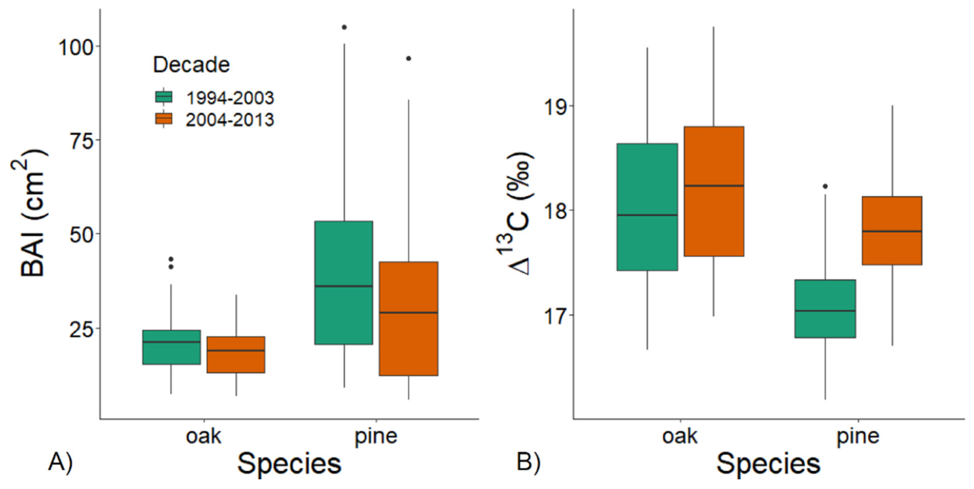
3.2. Individual Growth and Δ13C during Wet and Dry Decades

Medium-term responses in BAI and Δ13C were assessed for a wet (1994–2003) and a dry decade (2004–2013) separately. The ANCOVAs showed significant differences in BAI between species for both periods, with pines having higher growth than oaks overall (ca. 150%), but less growth was observed during the dry period, regardless of the species (around 19%; Figure 3a, Table 3). A higher Δ13C in oaks than in pines was also observed, particularly during the wet period (Figure 3b, Table 3). Contrary to expectations, Δ13C in pines increased significantly in the dry period as compared to the wet period (17.8 ± 0.05‰ vs. 17.1 ± 0.06‰, respectively; mean ± SE).
There was significant spatial variation of BAI in the stand (i.e., trees grew more along the X axis), and individual BAI variability was higher in pines than in oaks, with a ca. 4-fold higher variability not explained by the ANCOVA terms (or residual variance) in the former (Table 3). We also found significant inter- and intra-specific competition effects: both oaks and pines were marginally (negatively) affected by increasing local density of oaks (oak BA) during the dry period (Table 3). Additionally, pines (but not oaks) were negatively affected by the increasing presence of neighboring pines regardless of the period (as suggested by significant species × pine BA interactions; Table 3). There were no significant age effects on BAI (Table 3). Significant spatial patterns in Δ13C were also found along the main plot directions (e.g., trees exhibited less Δ13C along the X axis but higher Δ13C along the Y axis), and oaks showed a ca. 2-fold higher Δ13C residual variance than pines (Table 3). Similar to BAI, local density of oaks caused a marginal decrease in Δ13C in both species, but neither age nor pine local density significantly affected the ∆13C values (Table 3).

3.3. Association between Mid-Term Responses and Seasonal Water Uptake Patterns

Seasonal water uptake patterns (based on water stable isotopes) could be linked to medium-term tree responses in terms of Δ13C and, at least for oaks, BAI (Figure 4). In pines (Figure 4a), Δ13C of the wet period was negatively associated with δ18O of xylem water in October and November, corresponding to late drought and recovery during 2011, respectively. Additionally, Δ13C of the dry period was negatively associated with δ18O in September (early drought), showing weaker negative correlations with δ18O in October and November (late drought and recovery). No significant correlations were found between BAI of pines and δ18O of xylem water. In oaks (Figure 4b), Δ13C of both wet and dry decades was strongly negatively correlated with δ18O of xylem water in November (drought recovery) and, to a lesser degree, September (early drought). Δ13C of the wet decade also showed a weak negative association with δ18O in October (late drought). Unlike for pines, BAI of oaks showed significant negative associations with δ18O of xylem water, with the strongest correlation found between BAI of the dry decade and δ18O in November (recovery).

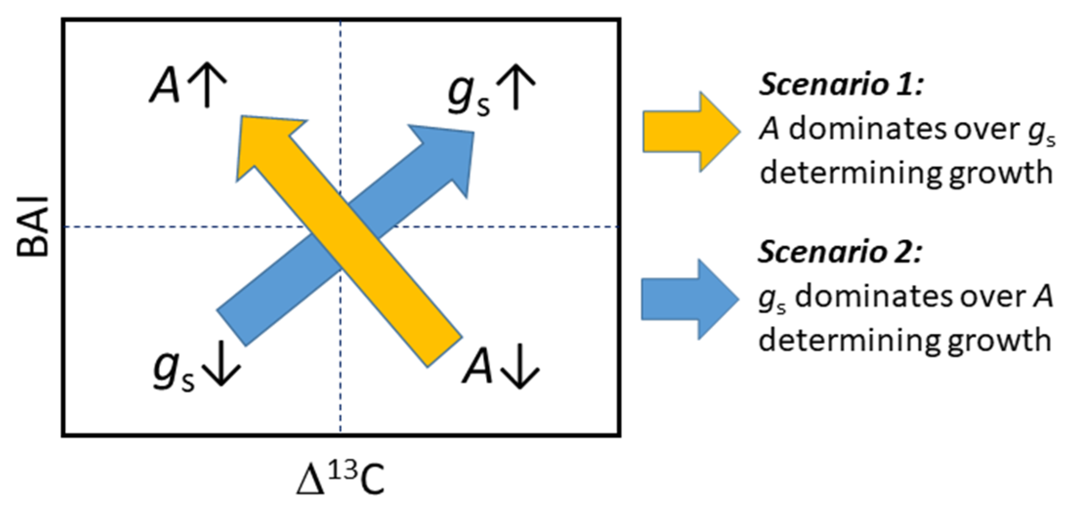
3.4. Interaction between Growth, Δ13C, and Water Uptake

Across individuals, we found that pines having high Δ13C (i.e., low WUEi) had lower BAI and there were no trees concurrently displaying high Δ13C and high BAI, whereas for oaks no significant trade-offs were observed (Figure 5). These results suggest that high WUEi was the obvious alternative to sustain a high growth for pines, especially during the wet period (1994–2003, Figure 5a), when the tightest association was found between BAI and Δ13C. Notably, the negative association between Δ13C and BAI was largely independent from the observed associations between Δ13C and δ18O, as evidenced by the color ramp in Figure 5, which shows δ18O values corresponding to November (values best linked to mid-term Δ13C variability).

4. Discussion

4.1. Climate Responses in Mixed Forests Are Modulated by Competition

Overall, radial growth of pines and oaks was driven by similar climate factors. In both cases, accumulated precipitation over the hydrological year (and, particularly, over winter–spring) positively influenced ring width, which was also (negatively) affected by spring temperature. The reliance of radial growth on winter precipitation has been widely described for holm oak, an archetypical example of a deep-rooted species which primarily relies on autumn–winter soil water recharge [11,34,35,36]. Conversely, this dependence is in principle less obvious for Aleppo pine, a more opportunistic, thermophillous species, than holm oak [37,38]. Different studies have concluded that summer dormancy may be mandatory or, at least, more restrictive in Aleppo pine, which forces this species to follow a bimodal growth pattern during spring and autumn [23,24]. In turn, this makes this species sensitive to winter rains during the first peak of secondary growth, particularly under relatively mild temperatures [24,39]. Indeed, a meta-analysis over the distribution range of Aleppo pine showed that this species is particularly sensitive to winter–spring precipitation, although this response shifts towards spring in more continental sites [40]. The continental nature of the site might explain the (unexpected) negative association between autumn precipitation and pine TRW, through an indirect effect of the negative association between autumn precipitation and temperature in October (r = −0.41, p = 0.081). During this month, average minimum temperatures (3.3 °C, range 1.6–4.8 °C, period 1994–2013) coincide with the minimum threshold for growth (see, e.g., [23]), making temperature more limiting than precipitation for the autumn growth peak of pine. Beyond these general, stand-level trends, we found that competition (as inferred from local density of each species) modulated the climatic response of oaks and, to a lesser extent, of pines. Oaks showed a time-lag in their growth responses under high density of pines, forcing them to become more sensitive to spring–summer precipitation and temperature. Conversely, the competition with other oaks increased their reliance on winter precipitation, and shifted the critical period for temperature from summer to spring. This could be partly a consequence of the faster reaction of Aleppo pine to precipitation pulses [23,24,37], which might reduce water availability for oaks during early spring. Another effect of the co-existence with pines is the reduction in light availability for oaks, since Aleppo pine usually grows taller than holm oak [10,19]. Although holm oak is a shade-tolerant species, this may cause a phenological delay and reduce their photosynthetic activity (and xylogenesis) during early spring [19]. Contrary to holm oak, Aleppo pine showed a moderate response to intra-specific competition, but increased its sensitivity to climate (particularly, to spring conditions) in the presence of oak neighbors. The lack of clear changes in climatic responses of pines under intra-specific competition agrees with a previous study showing different growth and physiological performance in dense versus open pine forests, but similar seasonal responses to climate [4]. Furthermore, this would agree with the proposed bimodal growth pattern in the pines, which would split the growing season into two main periods that respond to climate, reducing the temporal window of their climate responses compared with oaks [23,24,40]. On the other hand, the higher sensitivity of pines to precipitation and temperature under competition with oaks would agree with a higher drought stress of pines in mixed (as compared to monospecific) stands, as recently proposed [19].

4.2. Pines Modulate the Climatic Response of Oaks, but Oaks Rule in Long-Term Growth

The aforementioned changing response to climate drivers in the oaks under pine competition was not reflected in either accumulated growth (mean decadal BAI) or water-use efficiency (decadal ∆13C). Local density of pines had a negative effect only on pine BAI, particularly during the dry decade, whereas oak density negatively affected the BAI of both species during the dry decade. This would agree with the proposed increase in drought stress of water-saving, isohydric pines in the vicinity of more anisohydric oaks [5,19]. ∆13C was also not significantly affected by the local density of pines, but oak local density caused a reduction in ∆13C in both species. Again, this suggests an increase in the drought stress of pines in the presence of oaks, due to the greater ability of the latter to withdraw water from the soil. The lack of clear effects of pine density on ∆13C agrees with experimental studies on the effect of thinning in pure stands of Aleppo pine, which showed inconsistent effects on ∆13C in thinned stands, but a clear response in growth [41]. In this regard, our results mainly agree with our first hypothesis, as pine growth was more affected by oaks than vice versa, but do not support our second hypothesis, given the lack of a clear response in pine ∆13C.
We found higher and more variable growth rates in the pines, in agreement with previous results [23,35,38]. Pines also showed generally lower ∆13C than oaks, as expected for a more isohydric species [5,35,38]. However, Aleppo pine showed less individual variability in ∆13C than the holm oak, and higher ∆13C during the dry decade, contrary to what would be expected if changes in ∆13C were dominated by stomatal conductance. One potential explanation for this is that the radial growth of Aleppo pine is strongly restricted during very dry years, which may result in the dominance of the few favorable years of the decade in the isotopic signal. Additionally, growth during the dry years would take place only during the most favorable season, as highlighted by intra-annual studies [23,42,43,44], further diluting the drought signal in the ∆13C. However, this alone may not explain the observed increase in ∆13C during the dry decade. In this context, some studies have shown an increase in ∆13C after stress episodes causing pine decline [45,46,47], which could be attributed to a recovery at the leaf level due to hydraulic adjustments through defoliation and/or reduced needle growth, causing a decrease in leaf/sapwood area ratio [48,49,50]. Furthermore, experimental drought studies on Aleppo pine have shown that long-lasting droughts cause larger limitation to needle growth than to stem and root growth [50]. This alternative explanation, associated with losses in leaf area, seems particularly suitable for our case study, considering that 2004–2013 was a decade of persistent droughts, already causing visible symptoms of decay and tree mortality in our study site (seven of the originally marked pines died by 2014; [11]). Conversely, we did not observe clear evidence of decay in the oaks, contrary to what was reported in a nearby pure oak stand after the 2011 drought event [6]. Again, this would agree with the proposed positive effect of pines on the water status of oaks [19].

4.3. Trade-Offs and Synergies between Growth, Water-Use Efficiency, and Water Uptake

Overall, we found a negative association between BAI and ∆13C in pines, which could be interpreted as the result of higher WUEi (i.e., lower ∆13C) being determined by higher net assimilation, and thus linked with higher growth (first scenario in Figure 6). Under strong water availability gradients, most conifers (and Aleppo pine in particular) show a tight stomatal regulation, which usually results in a negative association between ∆13C and growth [4,35,51,52,53]. However, it has been observed that when light interception is the main limiting factor linked with competition, a negative association between ∆13C and growth may emerge [54]. Hence, a gradient of dominance–suppression may explain the observed trend within pines. On the other hand, a global positive association between genetic variation in WUEi and growth has been reported for conifers [55]. Therefore, this trend could be partly due to genetic variation among individuals within the study plot, with the fast-growing individuals showing a less conservative water use, and higher ∆13C. However, the latter might be highly speculative since Aleppo pine is one case for which intraspecific variation tends to show a trade-off between WUEi and growth [52,56]. Notably, this association was stronger during the wet decade, and restricted to the upper quantile of BAI and ∆13C, further supporting that it was independent from drought stress. In this regard, when comparing water uptake patterns with ∆13C, we found that individuals having access to deeper water sources (i.e., lower δ18O) also showed higher ∆13C, hence lower WUEi, but this was not reflected in BAI. In this case, this would fit with the second scenario shown in Figure 6, where WUEi and growth are dominated by stomatal conductance. Hence, we likely found two overlapping, independent sources of variation for ∆13C among pine individuals, which would explain these apparently contradictory results.
In the case of oaks, BAI and ∆13C were not correlated, but both showed a similar negative response to conspecific local density, aligned with the previously reported variation in water uptake, suggesting different levels of stress among individuals [11]. Notably, the strongest association between xylem water δ18O and both ∆13C and BAI was found considering the δ18O values obtained during drought recovery. As suggested by [11], hydraulic limitations after a long-lasting drought may limit the ability of oaks to uptake water from recent rain events. This would also agree with [24], which reported a faster reaction to autumn rains in the growth of pines than in the oaks. Unlike pines, leaf shedding is not among the mechanisms of holm oak to cope with drought, and this may cause substantial hydraulic damage to the stems under severe drought [21]. Furthermore, persistent drought has been shown to reduce vessel size in holm oak, reducing its vulnerability to cavitation, but restricting stem hydraulic conductivity [57]. In this regard, in oaks, the observed connection between short-term drought response (δ18O) and long-term effects (BAI, ∆13C) would be mainly driven by hydraulic limitations. Our findings confirm that intra-specific competition negatively affects the water status of oaks, but this is alleviated by the presence of pines, probably through a reduction in evaporative demand for the oaks growing under the canopy of pines [19].

5. Conclusions

Our results show that competition with pines modulates the (high-frequency) climate responses of oaks, whereas climate responses of pines are virtually insensitive to competition. Conversely, competition with pines does negatively affect pine growth in the mid-term (decadal), but has negligible effects on oaks. In turn, competition with oaks causes growth restrictions in both species, though mediated through different mechanisms. Pines under high oak competition would experience a more limited water availability in spring-summer, whereas oaks would show a slower recovery after drought. Hence, our results mainly agree with our first hypothesis, showing that the presence of pines had negligible effects on the oaks, while competition with oaks affected both species. On the contrary, our second hypothesis was not supported by the results, since ∆13C of pines was less sensitive to competition than oaks. Nevertheless, the competition with oaks increased WUEi in both species, further supporting our interpretation that growth response to competition was mainly driven by water availability. These results highlight the relevance of considering the role of mixed forests for forest resilience and future management in a climate change context, in which the Mediterranean might face an increase in drought frequency and water losses due to higher evapotranspiration as mean temperature increases.

Supplementary Materials

The full dataset is available in the supplementary file ‘Forests-1300818_dataset.xlsx’ https://www.mdpi.com/article/10.3390/f12081093/s1.

Author Contributions

Conceptualization, J.P.F., J.d.C. and J.V.; methodology, J.P.F., J.d.C. and T.A.S.; formal analysis, J.V., T.A.S. and J.P.F.; data curation, J.P.F. and J.d.C.; writing—original draft preparation, J.P.F.; writing—review and editing, J.P.F., T.A.S., J.d.C. and J.V.; funding acquisition, J.P.F. and J.V. All authors have read and agreed to the published version of the manuscript.

Funding

This research was funded by the Spanish Government through Projects CGL2011-26654 and RTI2018-094691-B-C31 (MCIU/AEI/FEDER, EU). J.P.F. was supported by Reference Group H09_20R (Gobierno de Aragón, Spain).

Data Availability Statement

The data presented in this study are available in the Supplementary Material.

Acknowledgments

The authors would like to thank P. Sopeña and M.J. Pau for technical assistance with sample preparation.

Conflicts of Interest

The authors declare no conflict of interest. The funders had no role in the design of the study; in the collection, analyses, or interpretation of data; in the writing of the manuscript, or in the decision to publish the results.

Appendix A

Table A1. Model parameters and determination coefficients (r2) for the estimation of historical climate values at Ulldemolins from long-term series of alternative meteorological stations. Tmax and Tmin, mean monthly maximum and minimum temperature, respectively; P, total monthly precipitation.
Station/VariableCommon PeriodnInterceptSloper2
Flix-Vinebre/Tmax2008–20191413.6220.9400.941
Flix-Vinebre/Tmin2008–2019141−6.1190.8440.915
Cabacés/P2008–20191415.1220.9520.847
Table A2. Additional indicators of the differences in precipitation between the two periods. P25, P50, and P75 stand for the 25%, 50%, and 75% percentiles, respectively; P < mean, percentage of years with precipitation below the long-term mean (520 mm); Pmin and Pmax, minimum and maximum annual precipitation.
PeriodP25P50P75P < meanPminPmax
Long-term
(1970–2019)
421 mm502 mm593 mm56%306 mm798 mm
Wet decade
(1994–2003)
498 mm598 mm676 mm30%409 mm744 mm
Dry decade
(2004–2013)
426 mm472 mm532 mm70%306 mm644 mm
Table A3. Analyses of covariance (ANCOVAs, full models) for log-transformed individual basal area increment (log(BAI)) and carbon isotope discrimination (Δ13C) during a wet (1994–2003) and a dry decade (2004–2013). Pine and oak BA, local density of pines and oaks, respectively; X and Y, Easting and Northing coordinates, respectively. Factors with p < 0.05 and p < 0.10 are highlighted in bold and italics, respectively.
log(BAI) (1994–2003)log(BAI) (2004–2013)Δ13C (1994–2003)Δ13C (2004–2013)
df.Fp > FFp > FFp > FFp > F
Species115.3<0.0019.80.00241.2<0.0018.20.007
X12.50.1186.00.0161.90.1731.90.178
Y11.50.2191.40.2352.80.1062.30.139
Age13.90.0511.90.1700.00.8520.00.934
Pine BA10.00.9580.50.4600.50.4880.90.357
Oak BA13.00.0893.10.0823.20.0833.90.058
Species × X10.20.6480.90.3424.40.0431.90.178
Species × Y12.10.1474.10.0461.90.1771.00.321
Species × Age10.40.5210.90.3530.70.4110.40.508
Species × Pine BA14.80.0326.50.0120.30.6110.50.471
Species × Oak BA10.20.6970.00.8440.10.7912.40.130

References

  1. Giorgi, F. Climate change hot-spots. Geophys. Res. Lett. 2006, 33, L08707. [Google Scholar] [CrossRef]
  2. Pausas, J.G.; Millán, M.M. Greening and browning in a climate change hotspot: The Mediterranean sasin. Bioscience 2019, 69, 143–151. [Google Scholar] [CrossRef] [Green Version]
  3. Valladares, F.; Benavides, R.; Rabasa, S.G.; Diaz, M.; Pausas, J.G.; Paula, S.; Simonson, W.D. Global change and Mediterranean forests: Current impacts and potential responses. In Forests and Global Change; Coomes, D.A., Burslem, D.F.R.P., Simonson, W.D., Eds.; Cambridge University Press: Cambridge, UK, 2014; pp. 47–75. [Google Scholar]
  4. Moreno-Gutiérrez, C.; Battipaglia, G.; Cherubini, P.; Saurer, M.; Nicolás, E.; Contreras, S.; Querejeta, J.I. Stand structure modulates the long-term vulnerability of Pinus halepensis to climatic drought in a semiarid Mediterranean ecosystem. Plant Cell Environ. 2012, 35, 1026–1039. [Google Scholar] [CrossRef] [PubMed]
  5. Klein, T.; Shpringer, I.; Fikler, B.; Elbaz, G.; Cohen, S.; Yakir, D. Relationships between stomatal regulation, water-use, and water-use efficiency of two coexisting key Mediterranean tree species. For. Ecol. Manag. 2013, 302, 34–42. [Google Scholar] [CrossRef]
  6. Barbeta, A.; Mejía-Chang, M.; Ogaya, R.; Voltas, J.; Dawson, T.E.; Peñuelas, J. The combined effects of a long-term experimental drought and an extreme drought on the use of plant-water sources in a Mediterranean forest. Glob. Chang. Biol. 2015, 21, 1213–1225. [Google Scholar] [CrossRef] [PubMed] [Green Version]
  7. Gracia, C.A.; Sabate, S.; Tello, E. Modelling the responses to climate change of a Mediterranean forest managed at different thinning intensities: Effects on growth and water fluxes. Impacts Glob. Chang. Tree Physiol. For. Ecosyst. 1998, 52, 243–252. [Google Scholar]
  8. de Dios, R.S.; Velázquez, J.C.; Ollero, H.S. Classification and mapping of Spanish Mediterranean mixed forests. IForest 2019, 12, 480–487. [Google Scholar] [CrossRef] [Green Version]
  9. Rivas-Martinez, S. Map of series, geoseries and geopermaseries of Spanish vegetation. Itinera Geobot. 2011, 18, 425–800. [Google Scholar]
  10. Zavala, M.A.; Espelta, J.M.; Retana, J. Constraints and trade-offs in Mediterranean plant communities: The case of holm oak-Aleppo pine forests. Bot. Rev. 2000, 66, 119–149. [Google Scholar] [CrossRef]
  11. del Castillo, J.; Comas, C.; Voltas, J.; Ferrio, J.P. Dynamics of competition over water in a mixed oak-pine Mediterranean forest: Spatio-temporal and physiological components. For. Ecol. Manag. 2016, 382, 214–224. [Google Scholar] [CrossRef] [Green Version]
  12. Filella, I.; Peñuelas, J. Partitioning of water and nitrogen in co-occurring Mediterranean woody shrub species of different evolutionary history. Oecologia 2003, 137, 51–61. [Google Scholar] [CrossRef] [PubMed]
  13. Moreno-Gutiérrez, C.; Dawson, T.E.; Nicolás, E.; Querejeta, J.I. Isotopes reveal contrasting water use strategies among coexisting plant species in a Mediterranean ecosystem. New Phytol. 2012, 196, 489–496. [Google Scholar] [CrossRef] [PubMed]
  14. Jucker, T.; Bouriaud, O.; Avacaritei, D.; Dǎnilǎ, I.; Duduman, G.; Valladares, F.; Coomes, D.A. Competition for light and water play contrasting roles in driving diversity-productivity relationships in Iberian forests. J. Ecol. 2014, 102, 1202–1213. [Google Scholar] [CrossRef] [Green Version]
  15. Grossiord, C.; Granier, A.; Ratcliffe, S.; Bouriaud, O.; Bruelheide, H.; Checko, E.; Forrester, D.I.; Dawud, S.M.; Finer, L.; Pollastrini, M.; et al. Tree diversity does not always improve resistance of forest ecosystems to drought. Proc. Natl. Acad. Sci. USA 2014, 111, 14812–14815. [Google Scholar] [CrossRef] [Green Version]
  16. Granda, E.; Rossatto, D.R.; Camarero, J.J.; Voltas, J.; Valladares, F. Growth and carbon isotopes of Mediterranean trees reveal contrasting responses to increased carbon dioxide and drought. Oecologia 2014, 174, 307–317. [Google Scholar] [CrossRef]
  17. Maestre, F.T.; Valladares, F.; Reynolds, J.F. The stress-gradient hypothesis does not fit all relationships between plant-plant interactions and abiotic stress: Further insights from arid environments. J. Ecol. 2006, 94, 17–22. [Google Scholar] [CrossRef]
  18. Zavala, M.A.; De La Parra, R.B. A mechanistic model of tree competition and facilitation for Mediterranean forests: Scaling from leaf physiology to stand dynamics. Ecol. Model. 2005, 188, 76–92. [Google Scholar] [CrossRef]
  19. De Cáceres, M.; Mencuccini, M.; Martin-StPaul, N.; Limousin, J.M.; Coll, L.; Poyatos, R.; Cabon, A.; Granda, V.; Forner, A.; Valladares, F.; et al. Unravelling the effect of species mixing on water use and drought stress in Mediterranean forests: A modelling approach. Agric. For. Meteorol. 2021, 296, 108233. [Google Scholar] [CrossRef]
  20. Comas, C.; del Castillo, J.; Voltas, J.; Ferrio, J.P. Point processes statistics of stable isotopes: Analysing water uptake patterns in a mixed stand of Aleppo pine and Holm oak. For. Syst. 2015, 24, e009. [Google Scholar] [CrossRef] [Green Version]
  21. Alonso-Forn, D.; Peguero-Pina, J.J.; Ferrio, J.P.; Mencuccini, M.; Mendoza-Herrer, Ó.; Sancho-Knapik, D.; Gil-Pelegrín, E. Contrasting functional strategies following severe drought in two Mediterranean oaks with different leaf habit: Quercus faginea and Quercus ilex subsp. rotundifolia. Tree Physiol. 2021, 41, 371–387. [Google Scholar] [CrossRef]
  22. Klein, T.; Hoch, G.; Yakir, D.; Körner, C. Drought stress, growth and nonstructural carbohydrate dynamics of pine trees in a semi-arid forest. Tree Physiol. 2014, 34, 981–992. [Google Scholar] [CrossRef] [Green Version]
  23. Campelo, F.; Gutiérrez, E.; Ribas, M.; Sánchez-Salguero, R.; Nabais, C.; Camarero, J.J. The facultative bimodal growth pattern in Quercus ilex–A simple model to predict sub-seasonal and inter-annual growth. Dendrochronologia 2018, 49, 77–88. [Google Scholar] [CrossRef]
  24. Campelo, F.; Ribas, M.; Gutiérrez, E. Plastic bimodal growth in a Mediterranean mixed-forest of Quercus ilex and Pinus halepensis. Dendrochronologia 2021, 67, 125836. [Google Scholar] [CrossRef]
  25. Palacio, S.; Azorín, J.; Montserrat-Martí, G.; Ferrio, J.P. The crystallization water of gypsum rocks is a relevant water source for plants. Nat. Commun. 2014, 5, 4660. [Google Scholar] [CrossRef] [Green Version]
  26. Martín-Gómez, P.; Barbeta, A.; Voltas, J.; Peñuelas, J.; Dennis, K.; Palacio, S.; Dawson, T.E.; Ferrio, J.P. Isotope-ratio infrared spectroscopy: A reliable tool for the investigation of plant-water sources? New Phytol. 2015, 207, 914–927. [Google Scholar] [CrossRef]
  27. Friedman, J.H. A Variable Span Smoother; Technical Report 5; Stanford University: Stanford, CA, USA, 1984. [Google Scholar] [CrossRef]
  28. Cook, E.R.; Krusic, P.J. Program ARSTAN: A Tree Ring Standardization Program Based on Detrending and Autoregressive Time Series Modeling, with Interactive Graphics; Columbia University: Palisades, NY, USA, 2005. [Google Scholar]
  29. Farquhar, G.D.; Ehleringer, J.R.; Hubick, K.T.; Ehleringer, R.; Hubic, K.T. Carbon Isotope Discrimination and Photosynthesis. Annu. Rev. Plant Physiol. Plant Mol. Bioi 1989, 40, 503–537. [Google Scholar] [CrossRef]
  30. Ferrio, J.P.; Araus, J.L.; Buxó, R.; Voltas, J.; Bort, J. Water management practices and climate in ancient agriculture: Inferences from the stable isotope composition of archaeobotanical remains. Veg. Hist. Archaeobot. 2005, 14, 510–517. [Google Scholar] [CrossRef]
  31. Verbeke, G.; Molenberghs, G. Linear Mixed Models for Longitudinal Data; Springer, Inc.: New York, NY, USA, 2000. [Google Scholar]
  32. Koenker, R. Quantreg: Quantile Regression. Available online: https://CRAN.R-project.org/package=quantreg (accessed on 15 May 2021).
  33. R Core Team. R: A Language and Environment for Statistical Computing; R Foundation for Statistical Computing: Vienna, Austria, 2021; Available online: https://www.R-project.org/ (accessed on 15 May 2021).
  34. Valentini, R.; Mugnozza, G.E.S.; Ehleringer, J.R. Hydrogen and Carbon Isotope Ratios of Selected Species of a Mediterranean Macchia Ecosystem. Funct. Ecol. 1992, 6, 627–631. [Google Scholar] [CrossRef]
  35. Ferrio, J.P.; Florit, A.; Vega, A.; Serrano, L.; Voltas, J. Δ13C and tree-ring width reflect different drought responses in Quercus ilex and Pinus halepensis. Oecologia 2003, 137, 512–518. [Google Scholar] [CrossRef]
  36. Gutiérrez, E.; Campelo, F.; Camarero, J.J.; Ribas, M.; Muntán, E.; Nabais, C.; Freitas, H. Climate controls act at different scales on the seasonal pattern of Quercus ilex L. stem radial increments in NE Spain. Trees-Struct. Funct. 2011, 25, 637–646. [Google Scholar] [CrossRef]
  37. Serre, F. The relation between growth and climate in Aleppo pine (Pinus halepensis). I. Methods. Cambial activity and climate. Oecologia Plant 1976, 11, 143–171. [Google Scholar]
  38. Del Castillo, J.; Aguilera, M.; Voltas, J.; Ferrio, J.P. Isoscapes of tree-ring carbon-13 perform like meteorological networks in predicting regional precipitation patterns. J. Geophys. Res. Biogeosci. 2013, 118, 352–360. [Google Scholar] [CrossRef] [Green Version]
  39. Liphschitz, N.; Lev-Yadun, S. Cambial activity of evergreen and seasonal dimorphics around the Mediterranean. IAWA Bull. NS 1986, 7, 145–153. [Google Scholar] [CrossRef]
  40. De Luis, M.; Čufar, K.; Di Filippo, A.; Novak, K.; Papadopoulos, A.; Piovesan, G.; Rathgeber, C.B.K.; Raventós, J.; Saz, M.A.; Smith, K.T. Plasticity in dendroclimatic response across the distribution range of Aleppo pine (Pinus halepensis). PLoS ONE 2013, 8, e83550. [Google Scholar] [CrossRef] [Green Version]
  41. Fernandes, T.J.G.; Del Campo, A.D.; Herrera, R.; Molina, A.J. Simultaneous assessment, through sap flow and stable isotopes, of water use efficiency (WUE) in thinned pines shows improvement in growth, tree-climate sensitivity and WUE, but not in WUEi. For. Ecol. Manag. 2016, 361, 298–308. [Google Scholar] [CrossRef]
  42. Forner, A.; Aranda, I.; Granier, A.; Valladares, F. Differential impact of the most extreme drought event over the last half century on growth and sap flow in two coexisting Mediterranean trees. Plant Ecol. 2014, 215, 703–719. [Google Scholar] [CrossRef] [Green Version]
  43. Klein, T.; Hemming, D.; Lin, T.; Grünzweig, J.M.; Maseyk, K.; Rotenberg, E.; Yakir, D. Association between tree-ring and needle δ13C and leaf gas exchange in Pinus halepensis under semi-arid conditions. Oecologia 2005, 144, 45–54. [Google Scholar] [CrossRef] [PubMed]
  44. Nicault, A.; Rathgeber, C.; Tessier, L.; Thomas, A. Observations on the development of rings of Aleppo pine (Pinus halepensis Mill.): Confrontation between radial growth, density and climatic factors. Ann. For. Sci. 2001, 58, 769–784. [Google Scholar] [CrossRef] [Green Version]
  45. Voltas, J.; Camarero, J.J.; Carulla, D.; Aguilera, M.; Ortiz, A.; Ferrio, J.P. A retrospective, dual-isotope approach reveals individual predispositions to winter-drought induced tree dieback in the southernmost distribution limit of Scots pine. Plant Cell Environ. 2013, 36, 1435–1448. [Google Scholar] [CrossRef]
  46. de Andrés, E.G.; Camarero, J.J. Disentangling mechanisms of drought-induced dieback in Pinus nigra arn. From growth and wood isotope patterns. Forests 2020, 11, 1339. [Google Scholar] [CrossRef]
  47. Petrucco, L.; Nardini, A.; Von Arx, G.; Saurer, M.; Cherubini, P. Isotope signals and anatomical features in tree rings suggest a role for hydraulic strategies in diffuse drought-induced die-back of Pinus nigra. Tree Physiol. 2017, 37, 523–535. [Google Scholar] [CrossRef]
  48. Galiano, L.; Martínez-Vilalta, J.; Lloret, F. Carbon reserves and canopy defoliation determine the recovery of Scots pine 4yr after a drought episode. New Phytol. 2011, 190, 750–759. [Google Scholar] [CrossRef] [PubMed]
  49. Peguero-Pina, J.J.; Alquézar-Alquézar, J.M.; Mayr, S.; Cochard, H.; Gil-Pelegrín, E. Embolism induced by winter drought may be critical for the survival of Pinus sylvestris L. near its southern distribution limit. Ann. For. Sci. 2011, 68, 565–574. [Google Scholar] [CrossRef]
  50. Klein, T.; Cohen, S.; Yakir, D. Hydraulic adjustments underlying drought resistance of Pinus halepensis. Tree Physiol. 2011, 31, 637–648. [Google Scholar] [CrossRef] [Green Version]
  51. Shestakova, T.A.; Camarero, J.J.; Ferrio, J.P.; Knorre, A.A.; Gutiérrez, E.; Voltas, J. Increasing drought effects on five European pines modulate Δ13C-growth coupling along a Mediterranean altitudinal gradient. Funct. Ecol. 2017, 31, 1359–1370. [Google Scholar] [CrossRef] [Green Version]
  52. Klein, T.; Di Matteo, G.; Rotenberg, E.; Cohen, S.; Yakir, D. Differential ecophysiological response of a major Mediterranean pine species across a climatic gradient. Tree Physiol. 2013, 33, 26–36. [Google Scholar] [CrossRef] [Green Version]
  53. Warren, C.R.; McGrath, J.F.; Adams, M.A. Water availability and carbon isotope discrimination in conifers. Oecologia 2001, 127, 476–486. [Google Scholar] [CrossRef]
  54. Mcdowell, N.; Brooks, J.R.; Fitzgerald, S.A.; Bond, B.J. Carbon isotope discrimination and growth response of old Pinus ponderosa trees to stand density reductions. Plant Cell Environ. 2003, 26, 631–644. [Google Scholar] [CrossRef]
  55. Fardusi, M.J.; Ferrio, J.P.; Comas, C.; Voltas, J.; de Dios, V.R.; Serrano, L. Intra-specific association between carbon isotope composition and productivity in woody plants: A meta-analysis. Plant Sci. 2016, 251, 110–118. [Google Scholar] [CrossRef] [Green Version]
  56. Voltas, J.; Chambel, M.R.; Prada, M.A.; Ferrio, J.P. Climate-related variability in carbon and oxygen stable isotopes among populations of Aleppo pine grown in common-garden tests. Trees-Struct. Funct. 2008, 22, 759–769. [Google Scholar] [CrossRef]
  57. Corcuera, L.; Camarero, J.J.; Gil-Pelegrín, E. Effects of a severe drought on Quercus ilex radial growth and xylem anatomy. Trees-Struct. Funct. 2004, 18, 83–92. [Google Scholar] [CrossRef]
Figure 1. Location of the study site and the meteorological stations used in this study. Map developed with QGIS 3.18.2-Zürich (https://qgis.org/es/site/, accessed on 20 December 2021). Background: ESRI Terrain (© OpenStreetMap contributors, https://www.openstreetmap.org/copyright, accessed on 15 May 2021) (upper panel); 2012 orthophotography from the public map server IGN-PNOA WMS (https://pnoa.ign.es, accessed on 15 May 2021; OrtoPNOA 2012 CC-BY 4.0 scne.es) (lower panel).
Forests 12 01093 g001
Figure 2. Simple (Pearson) correlation coefficients between linearly detrended time series of climate and indexed tree-ring chronologies (TRW) for the period 1994-2013. The relationships were evaluated for the whole stand (All) and for each local-density class, based on pine or oak local basal area (BA), as defined in Table 2. L, M, and H, low, medium, and high local density classes; Psep dec-1, precipitation during previous-year autumn recharge; Pjan mar, Papr may, Pjun aug, Psep oct, and Pyear, winter, spring, summer, autumn, and total precipitation in current calendar year, respectively; Poct-1 sep, precipitation during the hydrological year; Tjan mar, Tapr may, Tjun aug, Tsep oct, and Tyear, spring, summer, autumn, and annual mean temperature in current calendar year. Correlations with p < 0.05 and p < 0.10 are highlighted in bold and italics, respectively.
Forests 12 01093 g002
Figure 3. Boxplot for (A) individual basal area increment (BAI) and (B) carbon isotope discrimination (Δ13C) of oaks and pines during a wet (1994–2003, green boxes) and a dry decade (2004–2013, orange boxes). Boxes stand for the 25% (Q1), 50% (median) and 75% (Q3) percentiles, and whiskers indicate the highest and lowest value within ±1.5 fold of the inter-quantile range (Q3–Q1). Outliers beyond these limits are shown as individual dots.
Forests 12 01093 g003
Figure 4. Weighted simple (Pearson) correlation coefficients between either Δ13C or log-transformed BAI (corresponding to a wet (1994-2003) or a dry decade (2004-2013)) and seasonal values of δ18O of xylem water measured during a drought and recovery cycle in 2011. (A) Pines; (B) oaks. Correlations with p < 0.05 and p < 0.10 are highlighted in bold and italics, respectively. As a reference for water status, accumulated precipitation during the 30 days (Pmm-30d) preceding each xylem water sampling (dates: 26 May, 20 July, 9 September, 19 October, and 18 November 2011) is shown in the bottom panels.
Forests 12 01093 g004
Figure 5. Quantile regressions between Δ13C and BAI during a wet (1994-2003; left panels) and a dry decade (2004-2013; right panels). (A,B) Pines; (C,D) oaks. The lines indicate 0.75 quantile regressions, including p-values of the slope coefficient. Significant regressions are shown with continuous lines, non-significant regressions with dashed lines. Color ramp of the dots denotes δ18O values of xylem water measured in November of 2011.
Forests 12 01093 g005
Figure 6. Mechanistic interpretation of the association between growth (basal area increment, BAI) and carbon isotope discrimination (∆13C), as dominated by changes in either net assimilation (A) or stomatal conductance (gs).
Forests 12 01093 g006
Table 1. Annual and seasonal values of mean temperature and precipitation during the long-term reference period (1970–2019) and the two decades considered in this study: wet (1994–2003) and dry (2004–2013). Seasons were defined based on the typical phenology of the species [23], as follows: winter = January–March; spring = April–May; summer = June–August; autumn = September–October.
Mean Temperature/Precipitation
PeriodAnnualWinterSpringSummerAutumn
Long-term
(1970–2019)
13.5 °C/
520 mm
7.4 °C/
110 mm
13.8 °C/
119 mm
21.5 °C/
78 mm
16.7 °C/
117 mm
Wet decade
(1994–2003)
14.0 °C/
584 mm
8.2 °C/
101 mm
14.3 °C/
134 mm
21.9 °C/
76 mm
16.6 °C/
139 mm
Dry decade
(2004–2013)
13.8 °C/
479 mm
7.2 °C/
111 mm
14.4 °C/
123 mm
22.1 °C/
62 mm
17.2 °C/
102 mm
% change 1−1%/−18%−12%/+10%+1%/−8%+1%/−17%+4%/−26%
1 Change in temperature/precipitation during the dry decade, relative to the wet decade.
Table 2. Local density classes (low, medium, high) used to account for competition effects in the assessment of high-frequency climate responses. Mean local density (i.e., local stand basal area, BA) used as the grouping criteria for each class is highlighted in bold.
SpeciesGrouped byDensity ClassnLocal Density within a 5 m Radius (cm2)
Mean (Range)
Pine BAOak BA
PinePine BAlow261048 (0–1560)404 (0–1127)
medium231925 (1583–2310)570 (0–1156)
high263055 (2397–4467)492 (0–1042)
Oak BAlow271970 (414–3563)116 (0–259)
medium231818 (388–3640)449 (312–662)
high252238 (0–4467)918 (666–1156)
OakPine BAlow171191 (0–2053)430 (0–1049)
high162798 (2059–4217)378 (0–1261)
Oak BAlow171953 (0–3315)132 (0–357)
high161988 (357–4217)695 (360–1261)
Table 3. Analyses of covariance (ANCOVAs, simplified model) for log-transformed individual basal area increment (log(BAI)) and carbon isotope discrimination (Δ13C) during a wet (1994–2003) and a dry decade (2004-2013). Pine and oak BA, local density of pines and oaks, respectively; Res., residual variance; X and Y, Easting and Northing coordinates, respectively. AIC, Akaike Information Criterion for the full (AICfull) and simplified models (AICsim) is also shown. Factors with p < 0.05 and p < 0.10 are highlighted in bold and italics, respectively.
log(BAI) (1994–2003)log(BAI) (2004–2013)Δ13C (1994–2003)Δ13C (2004–2013)
df.Fp > FFp > FFp > FFp > F
Species114.6<0.0019.80.00251.2<0.00110.40.003
X1--6.00.0163.10.0873.40.073
Y1--1.40.2354.20.0483.40.075
Age11.80.1831.90.170----
Pine BA10.30.6110.50.460----
Oak BA1--3.10.0822.70.1083.30.076
Species × X1--0.90.3426.10.0183.00.090
Species × Y1--4.10.0461.70.2021.00.331
Species × Age10.10.8150.90.353----
Species × Pine BA14.50.0366.50.012----
Species × Oak BA1--0.00.8440.10.7872.310.137
AICsim 197.6-171.4166.9
AICfull 205.8212.4179.6181.0
Mean ± SERes. ± SEMean ± SERes. ± SEMean ± SERes. ± SEMean ± SERes. ± SE
Pines 32 ± 1.11.6 ± 1.126 ± 1.11.8 ± 1.117.07 ± 0.050.21 ± 0.0317.80 ± 0.050.20 ± 0.03
Oaks 20 ± 1.11.2 ± 1.117 ± 1.11.1 ± 1.018.17 ± 0.140.42 ± 0.1118.28 ± 0.140.40 ± 0.11
Publisher’s Note: MDPI stays neutral with regard to jurisdictional claims in published maps and institutional affiliations.

