
Before Becoming a World Heritage: Spatiotemporal Dynamics and Spatial Dependency of the Soundscapes in Kulangsu Scenic Area, China


1
School of Architecture and Urban-Rural Planning, Fuzhou University, Fuzhou 350108, China
2
Institute of Environmental Planning, Leibniz University Hannover, Herrenhäuser Str. 2, 30419 Hanover, Germany
3
Institute of Urban Environment, Chinese Academy of Sciences, Xiamen 361021, China
*
Author to whom correspondence should be addressed.
Forests 2022, 13(9), 1526; https://doi.org/10.3390/f13091526
Submission received: 24 August 2022
/
Revised: 8 September 2022
/
Accepted: 11 September 2022
/
Published: 19 September 2022
(This article belongs to the Special Issue Soundscape in Urban Forests)
Abstract
:Kulangsu is a famous scenic area in China and a World Heritage Site. It is important to obtain knowledge with regard to the status of soundscape and landscape resources and their interrelationships in Kulangsu before it became a World Heritage. The objective of this study was to explore the spatial dependency of the soundscapes in Kulangsu, based on the spatiotemporal dynamics of soundscape and landscape perceptions, including perceived sound sources, soundscape quality, and landscape satisfaction degree, and the spatial landscape characteristics, including the distance to green spaces, normalized difference vegetation index, and landscape spatial patterns. The results showed that perception of soundscape and landscape were observed in significant spatiotemporal dynamics, and the dominance of biological sounds in all sampling periods and human sounds in the evening indicated that Kulangsu scenic area had a good natural environment and a developed night-time economy, respectively. The green spaces and commercial lands may contribute to both the soundscape pleasantness and eventfulness. Moreover, the soundscape quality was dependent on the sound dominant degree and landscape satisfaction degree but not on the landscape characteristics. The GWR model had better goodness of fit than the OLS model, and possible non-linear relationships were found between the soundscape pleasantness and the variables of perceived sound sources and landscape satisfaction degree. The GWR models with spatial stationarity were found to be more effective in understanding the spatial dependence of soundscapes. In particular, the data applied should ideally include a complete temporal dimension to obtain a relatively high fitting accuracy of the model. These findings can provide useful data support and references for future planning and design practices, and management strategies for the soundscape resources in scenic areas and World Heritage Sites.
1. Introduction
Rapid urbanization has led to an increasing proportion of the population settling in cities worldwide [1]. Living in high-density built-up areas limits urban residents’ access to nature and may expose them to certain environmental hazards, such as noise pollution [2]. Scenic areas possess abundant natural and cultural landscapes as well as infrastructure and facilities for human activities [3], which is a critical vehicle for people to interact with natural environment. The scenic areas located in urban areas are an important and special urban green space (UGS), providing a variety of important ecosystem services to urban residents, such as air purification [4], biodiversity conservation [5], nature-based recreation [6], and noise and quiet reduction [7]. Furthermore, they can improve the quality of urban environments, promote sustainable lifestyles, contribute to human health and well-being [8], and even reduce mortality [9]. However, with the development of tourist industry, the conflicting interests e.g., between noise of tourist activities and experiencing the sounds of nature have become one of the focal issues in the management of scenic areas [10,11], because auditory perception is as important as visual perception in people’s visiting experience [12,13].
Currently, scholars no longer equate the good acoustic environment with simply reducing noise levels [14,15], but rather emphasize the importance of people’s subjective perception of the acoustic environment following the soundscape concept of ISO 12913-1 [16]. Against this backdrop, more and more studies have explored and focused on the human perceived acoustic environment [17,18]. However, exploring soundscapes needs a multi-faceted perspective because soundscape perception is associated with not only acoustic components but also non-acoustic factors [19]. Sound sources are the most basic and important acoustic components in creating soundscapes in urban areas [20], because the sound dominance in a soundscape is able to affect the spatiotemporal dynamics and the outcome of people’s perception of the soundscape [21,22]. Regarding non-acoustic factors, landscape compositions account for a high proportion of the influence on soundscape perception, with can be summarized as subjective and objective aspects [18]. The former is mainly due to people’s perception varied from landscape elements, such as naturalness [23], visual quality [24], urban contexts [25], features of landscape and architecture [17], audio-visual coherence [26], and infrastructure services [27]. The latter is related to the landscape characteristics, for example, accessibility [28], vegetation coverage [29], landscape spatial pattern [7], and biodiversity [30].
These relationships indicate that a soundscape may possess spatial dependencies on such factors. The spatial dependence is seen as a normal extension of the first law in geography [31]—“everything is related to everything else, but near things are more related than distant things”. It may occur due to the spatial dimensions with regard to social-cultural contexts and economic factors [32]. Previous studies found that the temporal dimension is also a critical aspect for exploring the spatial dependence, and neglecting the temporal characteristics could lead to a misunderstanding of the “real” measure of spatial dependence over time [33,34]. However, to date only a few studies have investigated spatial dependence of soundscape quality but with some deficiencies. For instance, Hong and Jeon [35] explored the spatial dependence of urban soundscapes, nonetheless, solely on the perceived sound sources. Rice et al. [36] explored the spatial dependence of noise abatement on the features of protected areas, but they did not consider people’s perception of the acoustic environment. In general, current studies have neither explored the spatial dependency of soundscape quality with the principal components, i.e., pleasantness and eventfulness [37], nor included variables in terms of landscape perception and green space features. Besides, the temporal characteristics of the spatial dependence of soundscape have not been effectively explored either. Exploring the spatial dependence of soundscape can clarify the interrelationship between soundscape perception and impact factors, which may help planners and managers identify the main disturbances to the acoustic environment in scenic areas and therefore find solutions and protection measures [35].
In 2016, Kulangsu was suggested as a cultural heritage by United Nations Educational, Scientific, and Cultural Organization (UNESCO), and subsequently was successfully listed as a World Heritage at the 41st World Heritage Congress in Krakow, Poland, in July 2017 [38]. Therefore, 2016 was a “landmark year” that represents a turning point for Kulangsu from China to the world. Kulangsu is a unique and historic international settlement, an important UGS, and a famous tourist attraction [39], the natural and cultural resources of which constitutes the unique soundscapes of outstanding universal value [40]. Unfortunately, such soundscapes are suffering from excessive disturbance and destruction by human activities, whether present, past, or even future. Accordingly, exploring the spatiotemporal dynamics of soundscapes and landscapes as well as the spatial dependence of soundscape quality in Kulangsu Island has significant implications for soundscape planning and management, and soundscape resources conservation, not only in UGS but also in the scenic area and even other similar World Heritage Sites. Given this importance, the objective of this study is (1) to visualize and analyze the spatiotemporal dynamics with regard to soundscape and landscape perception, as well as the spatial landscape features in Kulangsu Island; and (2) to examine the spatial dependence of soundscape quality on these compositions. To this end, both global and local spatial regression methods were employed.
2. Materials and Methods
2.1. Study Area
The study area is located on Kulangsu Island (Figure 1a), a World Heritage and one of the National 5A level tourist attractions in China. The area of it is about 1.92 km2, with a length of 2.3 km from north to south and 1.6 km from east to west. The green spaces occupied more than one-third of the island (Figure 1b), which was the highest percentage (32.36%) of land use type (according to 2017 land use vector data of Kulangsu Island obtained from Xiamen Municipal Natural Resources and Planning Bureau). The types of green space include parks, squares, and woodlands [41].
The present study was conducted from 17 July 2016, to 21 July 2016, in the application process of World Heritage. In July 2017, Kulangsu Island was officially inscribed on the World Heritage List. Based on the pilot study and relevant literature [7,12,42], 4 main-categories and 19 sub-categories sound sources were identified in the area (Table 1).
We selected 52 observation points according to the land use type, function, and accessibility, and interviewed random passersby by questionnaire surveys on site in the morning (8:00–11:00), afternoon (13:00–16:00), and evening (17:00–20:00) of the days. A team of 12 college students from landscape architecture faculty of Fuzhou University got involved to help conduct the field survey and distribute the questionnaire to random people in the study area. They were professionally trained before executing the field survey in order to ensure the quality of study. The data includes personal information and subjective perception ratings for the soundscape and landscape of the interviewees. A total of 703 valid questionnaires were returned, with 10 to 15 questionnaires on each sample site, indicating that enough and accurate results can be achieved [43,44]. The interviewees’ information is shown in Figure S1 (Supplementary Material). Analysis of the questionnaire data in SPSS 25.0 showed that the alpha coefficient was 0.86, indicating that the reliability of the questionnaire data was good and suitable for further analysis.
2.2. Data Collection
2.2.1. Soundscape and Landscape Perception
Participants were asked to evaluate the sound source, soundscape quality, and landscape satisfaction degree of the environment, based on perceived indicators using a Likert 5-point scale (Table 2).
2.2.2. Analysis of Landscape Characteristics
This study objectively quantifies the landscape features within Kulangsu in two aspects: (1) features of green spaces, including Distance to green spaces (DtGS) and Normalized difference vegetation index (NDVI), and (2) landscape spatial patterns, including patterns of the green space class and overall landscape. DtGS was calculated based on the “Euclidean distance” spatial analysis tool in GIS, which is measured in the projection unit of the raster and calculated from one cell center to the other cell center, and can objectively measure the spatial distance of the global scale [45], with the Equation (1) shows:
where (,) are the coordinates of one point, (,) are the coordinates of the other point; D is the Euclidean distance between (,) and (,).
We imported the collected Sentinel-2 level 2A images as an ensemble into the Google Earth Engine (GEE) JavaScript-based code editor environment [46], to calculate the value of NDVI for each time series image. Only images with less than 10% cloudiness in the study area were extracted, to ensure data integrity, and the calculated images were between March 2017 (the first Sentinel-2 available image in GEE) and January 2019. All data were top-of-atmosphere (TOA) images and had been atmospherically corrected [47]. The FMask algorithm [48] was used in multispectral instrument (MSI) data processed to identify cloud, cloud shadow, cirrus, and snow/ice observations. The NDVI values were calculated for each image element and a time series NDVI image collection with a spatial resolution of 10 m is generated. The calculation formula is shown in Equation (2):
where RED is the TOA values of the red band (630–680 nm); NIR is the TOA values of the near infrared band (845–885 nm). The NDVI takes values in the range of −1 to 1 [49].
To examine the landscape patterns, we considered landscape features in terms of area, density, shape, diversity, and aggregation on class and landscape levels [7,50]. Details of the calculated landscape spatial indices are shown in Supplementary Material (Table S1).
2.3. Mapping Process
Based on the questionnaire data, the mean values of ratings for soundscape and landscape perception were calculated for each observation point at each sampling time period, and the data were subsequently visualized in ArcGIS 10.7. By comparing the different interpolation methods provided in spatial analyst tools, the Inverse Distance Weighted (IDW) method was chosen to produce the soundscape and landscape perception maps to analyze their spatiotemporal dynamic characteristics. The IDW method is based on the spatial distance of the data points for weighted interpolation, and the closer the point is to the value, the greater the effect is. Conversely, the smaller the effect is [7,20,21].
The landscape index visualization is based on the moving window technique in Fragstats 4.2. The size and shape of the window can be defined by the user. The window is moved over each cell with positive value in the raster data, and the selected landscape index within the window is calculated. These values are then returned to the focal point (midpoint) of the cell, while a new continuous type of grid data is generated for each selected landscape index, where the cell values represent the “local neighborhood structure” [51]. According to the previous study [7], we set 175 m radius as the window size. In addition, we considered that Fragstats software gives negative values for cells near the edges and cells that are not fully included in the input grid window in the calculating process, which may lead to incomplete spatial data. Therefore, we created a buffer of the same size as the moving window (175 m) before inputting the grid data, thus minimizing the effect of boundary effects [52].
2.4. Statistical Analysis
(1) Principal Component Analysis (PCA). Based on the semantic attributes of the soundscape, the PCA method was applied to extract the principal components so as to obtain the determinants of overall soundscape quality. The eigenvalues of the extracted principal components were all greater than 1. The analysis was performed in SPSS 25.0.
(2) Multicollinearity Analysis. Before constructing a spatial regression model, it should be ensured that there is no multicollinearity problem among the independent variables included in the model [53]. The tolerance (TOL) and variance inflation factor (VIF) were used to perform the diagnosis of multicollinearity problems. TOL > 0.1 or VIF < 5 indicates that there is no multicollinearity problem between the analyzed [54]. Equations (3) and (4) were used to calculate TOL and VIF, respectively:
where is the coefficient of determination for the regression analysis on all other variables.
(3) Spatial Regression Model. Spatial regression models capturing spatial dependence were used to examine the effects of perceived sound sources, landscape satisfaction degree, and landscape characteristics on perceived soundscape quality within Kulangsu Island. Both the global spatial regression model—ordinary least squares (OLS) estimation model, and the local spatial regression model—geographically weighted regression (GWR) model were used (see Supplementary Material for details) [55], and the formulae of them are shown in Equations (5) and (6), respectively [56,57]. The explanatory ability and goodness of fit of these models were examined by the coefficient of determination (R2) and the Akaike Information Criterion (AIC) [58,59]. All operations were performed in ArcGIS 10.7.
where Yi is the dependent variable being explained; x1, x2… xn are the independent variable; β0 is constant; β1, β2… βn are variable coefficients; εi is the bias in estimating the coefficients.
where Yi is the explained dependent variable, xik is the independent variable at kth sample of I, (µi, vi) denotes the coordinates of the ith sample, β0 (µi, vi) denotes the intercept of the ith sample, βk (µi, vi) denotes the regression parameters of the ith sample, and εi denotes the residuals of the model at the ith sample in estimating the coefficients. All data were normalized to 0 to 1 prior to analysis.
3. Results
3.1. Spatiotemporal Dynamics of Soundscape and Landscape Perceptions
3.1.1. Soundscape Mapping
Figure 2 shows significant spatial and temporal variability in SDD for all four major sound sources. The SDD-GS is higher in the eastern and western parts, and relatively lower in the central part of the study area. The spatial distribution of SDD for BS, GS, and HS all changed significantly over time. The SDD-HS changed most significantly, and its high values covered almost entire area in the evening. However, the whole area was mainly dominated by BS in the morning. Compared with the SDD of the BS, GS, and HS, SDD-MS only changed slightly over time, and the overall distribution pattern was relatively stable. For the temporal variation of the mean values across land use types, the maximum mean values of SDD-BS in all periods were in the logistics and warehouse land. The mean values of SDD-GS were the always highest in development land, and the lowest in municipal land and logistics and warehouse land. The highest mean values of SDD-HS were found in logistics and warehouse land in P1 and P3, respectively, but in municipal utility land in P2. For SDD-MS, the highest mean values occurred in different land types in each period. The general trend of it was more diverse than the other three sounds.
PCA was used to extract the principal components of the six semantic attributes based on the varimax rotation method, for representing the soundscape quality. The Kaiser-Mayer-Olkin (KMO) test was 0.839 (KMO > 0.60), and the Bartlett’s test of sphericity was 0.000 indicating highly significant (p < 0.001), which means that the dataset was suitable for PCA. A total of two principal components were extracted: Component 1 (Pleasantness) and Component 2 (Eventfulness), which explained 41.8% and 38.8% of the variance in the semantic attribute dataset, respectively (Table 3). The results of this analysis are in good agreement with the two-dimensional model of perceived affective quality of soundscape (Pleasantness-Eventfulness) proposed in the previous study [37]. This model can provide comprehensive information on soundscape perception.
The values of pleasantness and eventfulness for each observing point were calculated in SPSS 25.0, and then visualized via ArcGIS 10.7 (Figure 3). Both components had significant spatiotemporal characteristics, and appeared to be similar in their distribution patterns. In general, the values of pleasantness and eventfulness in the study area showed low and high values in the north and south, respectively, in all periods. Regarding mean values of the components in different periods for each land use type, the trends of pleasantness and eventfulness were similar. The maximum and minimum values occurred in the same land use type in all periods. The maximum values were found in development land all the time. The minimum values were found in municipal utility land in P1, and in logistics and warehouse land in P2 and P3. The mean value of pleasantness first reduced and then improved in logistics and warehouse land, nonetheless, it had opposite trends in each of the rest land use types. The trend of eventfulness was different from that of pleasantness only in commercial and business facility land, which continued to decline over time.
3.1.2. Landscape Satisfaction Degree
Figure 4 indicates the spatiotemporal distribution of each landscape satisfaction degree indicator. Values of SNL, SLD, and SHB were relatively high, while that of SSF was significantly lower. The mapping results show that the spatial differences were pronounced for SLD and SHB, respectively, but that for SSF was relatively small. However, the spatial distribution patterns of them changed significantly with time. In P2, high values of SNL, SLD, and SHB covered almost the whole area. Nonetheless in P3, the high values of the first two weakened in the central and northern areas, but the high values of SHB still covered almost the whole area. The landscape satisfaction degree indicators showed presented the same trend of mean values in some land use types. The mean values of SNL and SLD in all types of land use, except for development land, showed the same trends. The trends of mean values of SHB and SSF were the same in all land use types. Both of their maximum mean values were found in logistics and warehouse land and development land in P2 and P3, respectively. The mean value of SVA increased and then decrease in all land use types, except for commercial and business facility land.
3.2. Spatial Landscape Characteristics
The DtGS and NDVI of the study area are shown in Figure 5. The result shows that the vast majority of the study area was close to green spaces (Figure 5a). The NDVI values showed low values in the central area (Figure 5b). The low NDVI values were also found in a few marginal areas of the study area. However, the NDVI values were generally at a high level, with more than 50% of the areas having the values over 0.5 [60], indicating a high vegetation coverage in Kulangsu Island.
Figure 6 shows the spatial distribution of the landscape indices at class level and landscape level. Except for SPLIT at the class level, all other landscape indices had significant spatial differences. For the landscape pattern of greenspaces, high values occurred at similar locations for CA and ED, but the latter covered a wider area. The high values of PD occurred only in a few areas near the northern and southern edges. The high values of IJI covered almost the entire area, while MESH and SPLIT showed lower levels within the area. For the landscape pattern of whole area, the high values of PD concentrated in the central and northern areas, and the high values of LSI were mainly found in the central-eastern area. The high values of SHDI were distributed similarly to those of IJI, which mainly gathered in the periphery of the study area, while the middle area showed a band of low values. SPLIT had a large area of low values in the area, and the high values of COHESION were found mainly in the central and southwestern areas.
3.3. Spatial Regression Models of Soundscape Quality
Spatial regression models, including OLS and GWR models, were built to examine the spatial dependence of soundscape quality (dependent variables) in Kulangsu Island. The explanatory (independent) variables include SDD of 4 main sound sources, landscape satisfaction degree, DtGS, NDVI, and landscape pattern indices.
3.3.1. Multicollinearity Diagnostic Results
To avoid possible covariance problems among the independent variables, we performed covariance diagnosis in the independent variables at the three periods and the whole day (Total), respectively, and selected the variables without multicollinearity in each period for the OLS regression. The results of multicollinearity diagnosis are shown in Table S2, Supplementary Material. Most variables passed the multicollinearity test, indicating rationality of the indicator selection. This analysis was performed in SPSS 25.0.
3.3.2. Global Spatial Regression Model
The OLS model used the data on each grid to build relationships between the independent and dependent variables (Table 4). None of the landscape indices significantly influenced the soundscape quality at all periods. Only the variables related to SDD and landscape satisfaction degree were significant for the soundscape quality. Pleasantness was only influenced by SLD in P3, and eventfulness was only significantly influenced by SLD in both P2 and P3. The included independent variables had better performances in explaining the pleasantness (R2 was 0.653 and 0.649, respectively) and eventfulness (R2 was 0.591 for both) in P1 and Total, compared with those in P2 and P3. Similarly, the results of the AIC demonstrate that the OLS models in P1 and Total had better fitting accuracy than those in P2 and P3.
3.3.3. Local Spatial Regression Model
The GWR model was to explore the spatial relationships between soundscape quality and the significant variables derived from the OLS model (Table 4). Before executing the GWR model, a kernel function needs to be selected for performing the geo-weighting algorithm, which is to estimate the local coefficients and their bandwidth sizes. There are two commonly used functions in GIS, namely the Gaussian fixed and adaptive kernel type. Based on the finding of previous study [35], we selected the Gaussian fixed kernel type to perform the GWR model.
The values of AIC of the GWR models in all period were significantly smaller than those of the OLS models (Table 5), indicating that the GWR model had better fitting results than the OLS model. The mean values of R2 of the GWR models were higher than those of the OLS models for the all periods, nonetheless, except for the pleasantness models in P1 and Total. As shown in Figure 7, the R2 spatial distributions of pleasantness model in P1, and both pleasantness and eventfulness models in Total were relatively stationary compared with those in P2 and P3. Also, Table 5 indicates that the results of R2 and AIC in P1 and Total were better than those in P2 and P3. These findings indicate that such spatial stationarity may achieve a better performance of the statistical model in terms of explanation of variance and goodness-of-fit.
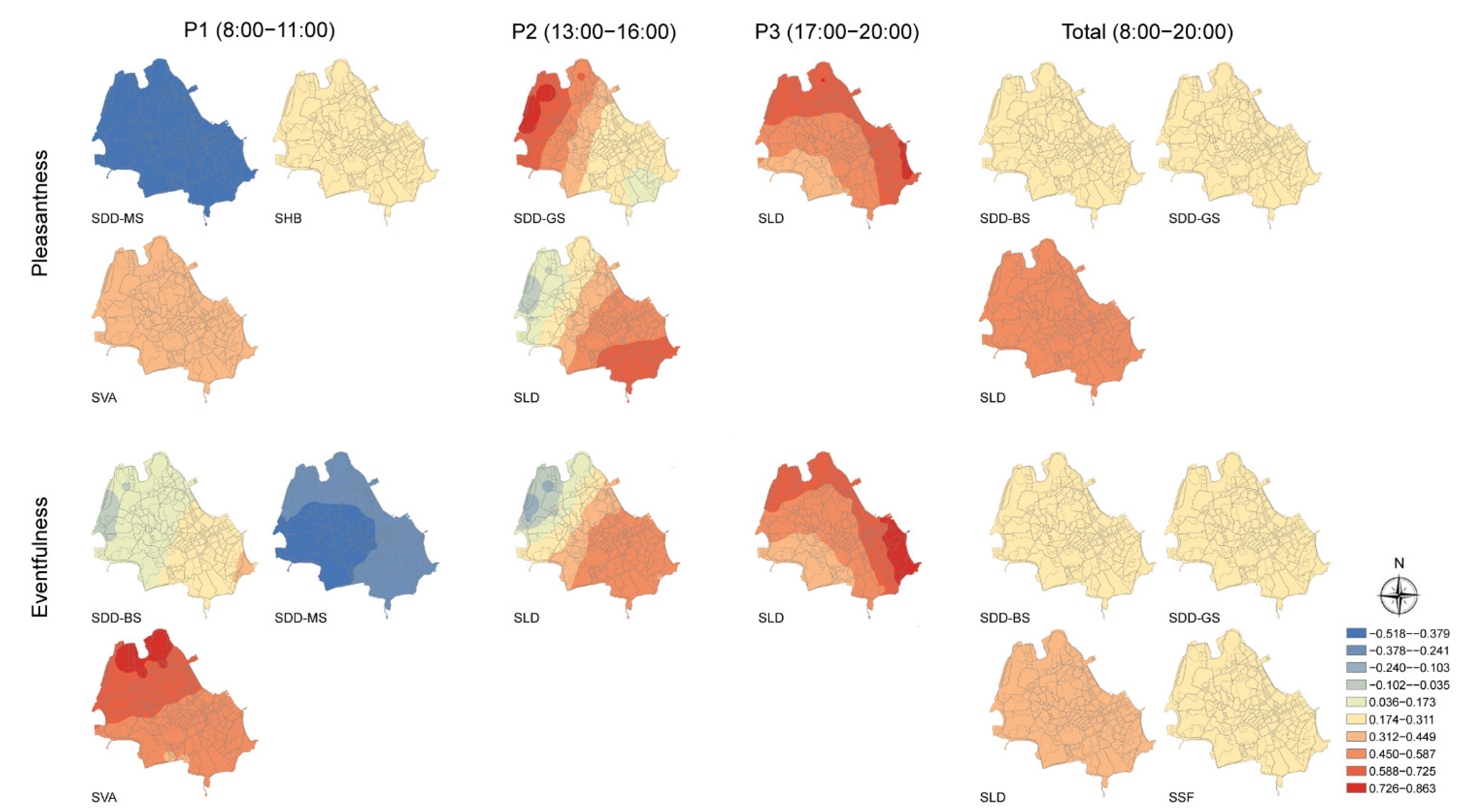
The spatial distribution of the coefficients of each independent variable are shown in Figure 8, the spatial stationarity also presented in pleasantness model in P1, and both pleasantness and eventfulness models in Total. In P1, SDD-MS and SVA exhibited the strongest negative and positive effects, respectively, on both pleasantness and eventfulness. In P2, SLD was positively related to both pleasantness and eventfulness in most areas, but their negative relationships appeared in few areas in the northwest. In addition, pleasantness was also positively influenced by SDD-GS, and the spatial differences were significant with the coefficients decreasing from northwest to southeast (from 0.808 to 0.139). In P3, both pleasantness and eventfulness were positively related to SLD only, with the coefficients increasing from southwest to northeast. In the model of Total, all included variables had positive relationships with pleasantness and eventfulness, respectively. SLD was the variable with strongest effects on pleasantness and eventfulness, respectively.
4. Discussion
4.1. Spatiotemporal Dynamics of Soundscape and Landscape in Kulangsu
The results of the present study showed that both soundscape and landscape perception in Kulangsu Island were characterized by significant spatiotemporal dynamics. In terms of perceived sound sources, we calculated and visualized the SDD for each main sound source, to present the dominance of them in different temporal and spatial dimensions in Kulangsu (Figure 2). The results demonstrated that BS and HS were the dominant sounds during the three sampling periods. The dominance of BS may imply the good quality of ecological environment within Kulangsu, which can attract various vocal organisms such as birds and insects to congregate and communicate here [61]. This was also reflected the high level of biodiversity in the island. Such abundance of natural resources also provides a good opportunity for tourism development, with many urban residents and tourists choosing to visit the area for e.g., nature-based recreation [62]. We speculate that this maybe one of the reasons why HS was another dominant sound.
We found that the HS-dominated area gradually expanded over time, and covered almost the entire area in the evening (Figure 2), indicating that this period was the most intensive period for people’s activities. This survey was conducted during the summer of July, which is generally the hottest period of the year in Xiamen [63]. Accordingly, we speculate that one reason for this phenomenon may be due to the higher thermal comfort in the evening, compared to the built-up area. This is probably due to the good vegetation condition in Kulangsu, which has a significant effect on reducing temperature thus creating a comfortable microclimate. Generally, such cooling effects were most pronounced in the evening [64]. Another reason may be the development of the night-time economy in China in recent years, which has led to a new urban living pattern dominated by night-time entertainment activities [65].
In the analysis of SDD mean values of the sound sources for different land use types (Figure 2), high SDD of BS and HS unexpectedly appeared several times in logistics and warehouse land. We suspect that this may be because this type of land use was generally small in size and surrounded by large areas of green spaces. This also potentially reflects that both animals and visitors were more willing to get close to the natural landscapes. The high GS-SDD mean values were mainly found in development land. This may be due to the harbors and waterfront spaces that were close to the sea in such land use type and therefore the GS especially water and wave sounds were more dominant. Such results are similar to the findings of previous studies located in coastal areas [66].
A similarity was found in the spatiotemporal distribution patterns of pleasantness and eventfulness of the soundscape (Figure 3), which implies they may be potentially interrelated. This finding is the same as previous soundscape studies located in urban built-up areas and urban forests [20,22]. For mean values of pleasantness and eventfulness across land use types (Figure 3), the maximum values of them were always found in development land, and mainly concentrated in the south according to the mapping result. This is possibly because the development land to the south were close to large areas of green spaces and commercial lands, and therefore subject to the “radiation effect” from such land types. The development land, on the other hand, were relatively smaller and thus may receive higher aggregated values of pleasantness and eventfulness. Another possible reason was that the development land encompassed many waterfront spaces where people prefer to stay, to experience nature and response higher values of pleasantness. Moreover, the consequent increase in foot traffic may also lead to high values of eventfulness [67].
As for landscape satisfaction degree, we found that the spatiotemporal distribution patterns of SNL, SLD, SHB, and SVA were similar to those of pleasantness and eventfulness in P1, but they were relatively different in P2 and P3 (Figure 3 and Figure 4). This finding suggests that the harmony or congruency between the soundscapes and landscapes in Kulangsu was still deficient especially in the afternoon and evening, and therefore it has room to improve in future landscape planning and design. We speculate that this audio-visual inconsistency may be due to the increasing spatial dominance of HS in these periods (Figure 2), which negatively affected the audio-visual perception [68]. Regarding the spatiotemporal distribution of SSF, it was significantly lower compared to the other landscape perception indicators. However, the distribution pattern of SSF was also similar to those of pleasantness and eventfulness in the morning and afternoon (Figure 3 and Figure 4). This similarity indicates that people may prefer to use these service facilities especially in these two periods. We suppose that this is because the temperatures in daytime are generally high in Kulangsu. This finding is also in line with the results of the previous study, which found infrastructure and facilities were an important factor contributing to the soundscape quality in scenic areas [27].
The analysis of “objective” landscape characteristics also illustrates the superior natural environmental characteristics of Kulangsu (Figure 5 and Figure 6), which was consistent with the finding derived from the spatiotemporal distribution of SDD-BS (Figure 2). These results indicated that Kulangsu had good green space accessibility and a high proportion of vegetation cover, which allows visitors to easily approach and experience nature and contributes to the comfortable microclimate here [60]. We found that although the high values of SDD-BS appeared in different areas over time, they almost always fell in the areas with low DtGS or high NDVI, indicating the interrelationship between biological sounds and green space features. Regarding the landscape pattern, the results of class metrics indicate that the green space patches were large and morphologically intact, with a high degree of connectivity, and did not have significant fragmentation. In addition to SPLIT, the spatial distributions of CA, PD, ED, IJI, and MESH were more or less similar to those of pleasantness and eventfulness in the three periods, suggesting that diverse and coherent structure of green space patches may contribute to soundscape quality [69]. Based on the results of the landscape metrics, we found that the structure of the patches in the center of Kulangsu was more complex and homogeneous, and the connectivity between patches was good. This may be due to the high density of historical architectures in the central area [70], but such buildings still maintain a good continuity. The edge of the study area, on the other hand, had a richer patch composition and different types of patches may be interspersed between similar patches. We found that this complexity tends to accompany areas where commercial land occurred. Based on such, we suggest that the remediation planning of scenic areas could focus on preventing the fragmentation effects on the landscape especially from dispersed commercial activities [71].
4.2. Spatial Dependencies of Soundscape Quality
Most indicators with regard to perceived sound sources, landscape satisfaction degree, the features of green spaces, and landscape patterns passed the test of multicollinearity on explaining the soundscape quality (Table S2), and then included in the OLS and GWR models. Interestingly, the results of OLS models (Table 4) show that the soundscape quality had no spatial dependence on all objective landscape characteristics, namely DtGS, NDVI, and landscape metrics on class and landscape levels. Both pleasantness and eventfulness of the soundscape were significantly dependent on the perceptual indicators of soundscape and landscape, i.e., SDD-BS, SDD-GS, SDD-MS, SLD, SHB, and SSF, in different periods. This finding was not exactly the same as previous studies on the relationship between soundscape elements and landscape patterns [7,72]. We speculate that this discrepancy may arise from two aspects. On the one hand, the research objectives and methods were different. The present study aimed to explore the spatial dependence of soundscape quality on many types of variables rather than the correlations between two variables. The spatial dependence can indicate the propensity for nearby locations to interact and share similar properties, which is also an essential part of modeling soundscape [35]. Therefore, the regression model accounting for the spatial dependence can explain more about the relationships between the dependent and independent variables, and predict the dependent variable based on such, while the correlation does not necessarily imply causation [73]. On the other hand, the study area was different. Our study was devoted to exploring the soundscape and landscape resources of the Kulangsu scenic area, whereas the previous studies were in a multifunctional urban area [7,20,72]. Kulangsu Scenic Area is rich in natural and cultural resources and locally distinctive sound sources, which is basically different from the urban area.
The result of soundscape spatial dependency on SDD-BS, SDD-GS, and SDD-MS suggests that introducing more birdsongs and vegetation sounds, through enriching the vegetation types and density, may contribute to the biodiversity and reduction of mechanical noise [74], therefore improving the pleasure and structure diversity of the soundscape [37]. Besides, according to the dependence on SLD and SHD, the soundscape quality can also be enhanced by optimizing the spatiotemporal features of landscape design, with regard to the lightscape (especially in the evening) and cultural innovation [24,75]. For instance, adding interesting lightscapes designed according to the natural and cultural environment characteristics of Kulangsu. The type and application of the light sources should be able to integrate into but not affect the natural environment [76]. Furthermore, the historical culture of Kulangsu can be combined with modern elements to revitalize old buildings by injecting new functions, such as cultural and creative business or exhibitions [77]. Also, the “Piano Island”, one of the famous titles of Kulangsu, can be used to create e.g., a theme-specific “musical environment” in different public open spaces by combining classical and contemporary featured piano music. The significant dependency of soundscape quality on the landscape perception indicators implies that only considering the effects of sound features on soundscape quality was insufficient in the past study [35]. This result also proves that the landscape compositions are indispensable factors in creating a soundscape [17,43]. The temporal differences of spatial dependence of the soundscape in Kulangsu can contribute specific information to the soundscape planning and design strategies for scenic areas and Heritage Site.
The GWR model was found to have a better goodness-of-fit than the OLS model for all periods according to the results of AIC, which was consistent with the previous study [35]. However, the R2 results of GWR model performing pleasantness in P1 and Total were lower than those of OLS model (Table 4 and Table 5). Interestingly, the spatially stationary relationships were found in the results of R2 and coefficients of the variables in pleasantness model in the morning and both pleasantness and eventfulness models in total dataset, respectively (Figure 7 and Figure 8). This finding suggests that the pleasantness models had better fitting accuracy if they were spatially stationary, but the explanatory power of the regression line for the dependent variable became weaker, which implies that the nonlinear relationship may be able to better explain the spatial dependence of soundscape pleasantness. This is also a good proof that the spatial stationarity helps to verify and select the suitable statistical methods in predicting variables [78,79]. As shown in Figure 7 and Figure 8, the total dataset models of pleasantness and eventfulness exhibited the best spatial stationarity, indicating the data used should ideally be of a time-varying nature that may contain as complete a temporal dimension as possible. For instance, the collected data should ideally cover morning, afternoon, evening, and even in the night or early morning.
4.3. Limitations and Future Studies
The limitations of the present study may mainly stem from the data collected and the model employed. Although vegetation coverage was considered in this study, the classification of green spaces was not in sufficient detail in terms of the vegetation type. The outcomes may therefore vary due to more detailed classification of vegetation cover. However, a high spatial resolution vegetation type data in China is difficult to obtain in general. Future studies are suggested to utilize data regarding vegetation cover types, such as coniferous forests, deciduous forests, shrubs, and grasslands, to explore the spatial relationship between their features and soundscape quality.
Moreover, the questionnaire data collected in 2016 was not up-to-date, nonetheless such data was still of research interest and significance, because this investigation can provide valuable historical research data for further exploring the environmental changes and soundscape planning and management. Given this importance, we suggest that future research could explore the spatiotemporal evolution of soundscape quality in Kulangsu in conjunction with the results of the present study. Based on e.g., the concept of DPSIR model [80], it is possible to predict the future state of soundscape resources in landscape planning.
The spatial model used in this study was based on a linear regression algorithm. Therefore, although the results indicated that landscape characteristics did not have significant effects on soundscape quality, this does not account for the possible non-linear relationships between these variables [81]. It has been proposed that the non-linear models may be able to explain soundscape perception better than the linear models [82]. However, the non-linear prediction models related to soundscape are still in their infancy, and most of them are only able to predict the values of output variables without spatiotemporal dynamic features [22,83,84]. Based on such, we recommend future studies could use the non-linear models to explore the soundscape spatiotemporal properties and to predict soundscape perception based on such. The models, such as the cellular automata, artificial neural networks, and Fuzzy-logic models [85,86]. Although the linear model is not perfect, the spatial regression model used in this study still presented a relatively better performance in spatially explaining the soundscape quality than the conventional regression model [20].
5. Conclusions
This study provided indispensable data with regard to the spatiotemporal dynamics of soundscape and landscape perception as well as the spatial landscape characteristics in Kulangsu. Furthermore, the spatial dependence of soundscape quality was examined. We found that sound dominant degree, soundscape quality, and landscape satisfaction degree all showed high spatiotemporal dynamics, and the distance to greenspaces, NDVI, and landscape patterns presented obviously spatial variations. Moreover, soundscape quality had spatial dependence on the sound dominant degree and landscape satisfaction degree, but not on the objective landscape characteristics. Such spatial dependence of soundscape quality provides useful suggestions for the design of soundscape and landscape. The GWR model had better goodness-of-fit than the OLS model, and the results with spatial stationarity of the GWR models suggest that applied data should consider as complete a time dimension as possible in exploring the spatial dependence of soundscape quality, which also guidance for soundscape modeling. The findings of this study will allow landscape planners to determine what factors the quality of a soundscape depends on, which gives a relatively comprehensive consideration of selected indicators for modeling soundscapes. They are also meaningful for the bringing soundscape evaluation into planning and design practices, especially for the development of specific planning goals and design strategies, which aim to protect, restore, and optimize the soundscape resources in the scenic areas and World Heritage Sites.
Supplementary Materials
The following supporting information can be downloaded at: https://www.mdpi.com/article/10.3390/f13091526/s1, Figure S1: Social/demographical/behavioral information of the interviewees; Table S1: Calculated landscape spatial indices at class and landscape levels; Table S2: Results of multicollinearity diagnosis for pleasantness and eventfulness at each sampling period; detailed concepts and definition in the statistical analysis. Reference [87] is cited in the supplementary materials.
Author Contributions
Conceptualization, Z.C., T.-Y.Z. and J.L.; methodology, Z.C. and J.L.; Software, Z.C. and T.-Y.Z.; validation, Z.C., T.-Y.Z., J.L. and X.-C.H.; formal analysis, Z.C. and T.-Y.Z.; investigation, Z.C. and T.-Y.Z.; resources, Z.C., T.-Y.Z. and J.L.; data curation, Z.C. and T.-Y.Z.; writing—original draft preparation, Z.C.; writing—review and editing, Z.C. and J.L.; visualization, Z.C. and T.-Y.Z.; supervision, J.L.; project administration, Z.C., J.L. and X.-C.H.; funding acquisition, J.L. and X.-C.H. All authors have read and agreed to the published version of the manuscript.
Funding
This research was funded by the National Natural Science Foundation of China (51508101 and 52208052), Fujian Provincial Department of Science & Technology (2017J01694), and the Program of Humanities and Social Science Research Program of Ministry of Education of China (21YJCZH038).
Data Availability Statement
Data available on request due to restrictions, e.g., privacy or ethical.
Acknowledgments
The first author, Zhu Chen, would like to thank the China Scholarship Council for the support of a doctoral scholarship (grant number: 202108080105). All the authors would like to thank the anonymous reviewers for their valuable comments, which have greatly improved the quality of this paper. We thank Christina von Haaren and Johannes Hermes for their very helpful suggestions in this paper.
Conflicts of Interest
The authors declare no conflict of interest.
References
- Zlotnik, H. World urbanization: Trends and prospects. In New Forms of Urbanization; Routledge: London, UK, 2017; pp. 43–64. ISBN 1315248077. [Google Scholar]
- Margaritis, E.; Kang, J. Relationship between urban green spaces and other features of urban morphology with traffic noise distribution. Urban For. Urban Green. 2016, 15, 174–185. [Google Scholar] [CrossRef]
- Zhang, Y.; Han, M.; Chen, W. The strategy of digital scenic area planning from the perspective of intangible cultural heritage protection. EURASIP J. Image Video Process. 2018, 2018, 130. [Google Scholar] [CrossRef]
- Liu, H.-L.; Shen, Y.-S. The impact of green space changes on air pollution and microclimates: A case study of the Taipei metropolitan area. Sustainability 2014, 6, 8827–8855. [Google Scholar] [CrossRef]
- Gao, T.; Liu, F.; Wang, Y.; Mu, S.; Qiu, L. Reduction of atmospheric suspended particulate matter concentration and influencing factors of green space in urban forest park. Forests 2020, 11, 950. [Google Scholar] [CrossRef]
- Wen, C.; Albert, C.; von Haaren, C. The elderly in green spaces: Exploring requirements and preferences concerning nature-based recreation. Sustain. Cities Soc. 2018, 38, 582–593. [Google Scholar] [CrossRef]
- Liu, J.; Kang, J.; Behm, H.; Luo, T. Landscape spatial pattern indices and soundscape perception in a multi-functional urban area, Germany. J. Environ. Eng. Landsc. Manag. 2014, 22, 208–218. [Google Scholar] [CrossRef]
- WHO. Urban Green Spaces: A Brief for Action; World Health Organization: Geneva, Switzerland, 2017. [Google Scholar]
- Vienneau, D.; de Hoogh, K.; Faeh, D.; Kaufmann, M.; Wunderli, J.M.; Röösli, M.; SNC Study Group. More than clean air and tranquillity: Residential green is independently associated with decreasing mortality. Environ. Int. 2017, 108, 176–184. [Google Scholar] [CrossRef]
- Herrera-Montes, M.I. Protected area zoning as a strategy to preserve natural soundscapes, reduce anthropogenic noise intrusion, and conserve biodiversity. Trop. Conserv. Sci. 2018, 11, 1940082918804344. [Google Scholar] [CrossRef]
- Miller, N.P. US National Parks and management of park soundscapes: A review. Appl. Acoust. 2008, 69, 77–92. [Google Scholar] [CrossRef]
- Liu, J.; Xiong, Y.; Wang, Y.; Luo, T. Soundscape effects on visiting experience in city park: A case study in Fuzhou, China. Urban For. Urban Green. 2018, 31, 38–47. [Google Scholar] [CrossRef]
- Li, H.; Lau, S.-K. A review of audio-visual interaction on soundscape assessment in urban built environments. Appl. Acoust. 2020, 166, 107372. [Google Scholar] [CrossRef]
- Aletta, F.; Kang, J.; Axelsson, Ö. Soundscape descriptors and a conceptual framework for developing predictive soundscape models. Landsc. Urban Plan. 2016, 149, 65–74. [Google Scholar] [CrossRef]
- Hong, J.Y.; Ong, Z.-T.; Lam, B.; Ooi, K.; Gan, W.-S.; Kang, J.; Feng, J.; Tan, S.-T. Effects of adding natural sounds to urban noises on the perceived loudness of noise and soundscape quality. Sci. Total Environ. 2020, 711, 134571. [Google Scholar] [CrossRef]
- ISO 12913-1:2014; Acoustics-Soundscape-Part 1: Definition and Conceptual Framework. ISO Genebra: Vernier, Switzerland, 2014.
- Liu, J.; Yang, L.; Xiong, Y.; Yang, Y. Effects of soundscape perception on visiting experience in a renovated historical block. Build. Environ. 2019, 165, 106375. [Google Scholar] [CrossRef]
- Chen, Z.; Hermes, J.; Liu, J.; von Haaren, C. How to integrate the soundscape resource into landscape planning? A perspective from ecosystem services. Ecol. Indic. 2022, 141, 109156. [Google Scholar] [CrossRef]
- Hong, J.Y.; Lam, B.; Ong, Z.-T.; Ooi, K.; Gan, W.-S.; Kang, J.; Yeong, S.; Lee, I.; Tan, S.-T. Effects of contexts in urban residential areas on the pleasantness and appropriateness of natural sounds. Sustain. Cities Soc. 2020, 63, 102475. [Google Scholar] [CrossRef]
- Hong, J.Y.; Jeon, J.Y. Relationship between spatiotemporal variability of soundscape and urban morphology in a multifunctional urban area: A case study in Seoul, Korea. Build. Environ. 2017, 126, 382–395. [Google Scholar] [CrossRef]
- Liu, J.; Kang, J.; Luo, T.; Behm, H.; Coppack, T. Spatiotemporal variability of soundscapes in a multiple functional urban area. Landsc. Urban Plan. 2013, 115, 1–9. [Google Scholar] [CrossRef]
- Hong, X.-C.; Wang, G.-Y.; Liu, J.; Song, L.; Wu, E.T.Y. Modeling the impact of soundscape drivers on perceived birdsongs in urban forests. J. Clean. Prod. 2021, 292, 125315. [Google Scholar] [CrossRef]
- Watts, G.; Marafa, L. Validation of the tranquillity rating prediction tool (TRAPT): Comparative studies in UK and Hong Kong. Noise Mapp. 2017, 4, 67–74. [Google Scholar] [CrossRef]
- Hong, X.-C.; Wang, G.-Y.; Liu, J.; Dang, E. Perceived Loudness Sensitivity Influenced by Brightness in Urban Forests: A Comparison When Eyes Were Opened and Closed. Forests 2020, 11, 1242. [Google Scholar] [CrossRef]
- Hong, J.Y.; Jeon, J.Y. Influence of urban contexts on soundscape perceptions: A structural equation modeling approach. Landsc. Urban Plan. 2015, 141, 78–87. [Google Scholar] [CrossRef]
- Kogan, P.; Gale, T.; Arenas, J.P.; Arias, C. Development and application of practical criteria for the recognition of potential Health Restoration Soundscapes (HeReS) in urban greenspaces. Sci. Total Environ. 2021, 793, 148541. [Google Scholar] [CrossRef]
- Xiong, Y.; Yang, L.; Wang, X.; Liu, J. Mediating effect on landscape experience in scenic area: A case study in Gulangyu Island, Xiamen City. Int. J. Sustain. Dev. World Ecol. 2020, 27, 276–283. [Google Scholar] [CrossRef]
- Votsi, N.-E.P.; Drakou, E.G.; Mazaris, A.D.; Kallimanis, A.S.; Pantis, J.D. Distance-based assessment of open country Quiet Areas in Greece. Landsc. Urban Plan. 2012, 104, 279–288. [Google Scholar] [CrossRef]
- Dzhambov, A.M.; Markevych, I.; Tilov, B.; Arabadzhiev, Z.; Stoyanov, D.; Gatseva, P.; Dimitrova, D.D. Lower noise annoyance associated with GIS-derived greenspace: Pathways through perceived greenspace and residential noise. Int. J. Environ. Res. Public Health 2018, 15, 1533. [Google Scholar] [CrossRef]
- Gunnarsson, B.; Knez, I.; Hedblom, M.; Sang, Å. Effects of biodiversity and environment-related attitude on perception of urban green space. Urban Ecosyst. 2017, 20, 37–49. [Google Scholar] [CrossRef]
- Tobler, W.R. A computer movie simulating urban growth in the Detroit region. Econ. Geogr. 1970, 46, 234–240. [Google Scholar] [CrossRef]
- Anselin, L. Spatial Econometrics: Methods and Models; Springer Science & Business Media: New York, NY, USA, 1988; ISBN 9024737354. [Google Scholar]
- Dubé, J.; Legros, D. A spatio-temporal measure of spatial dependence: An example using real estate data. Pap. Reg. Sci. 2013, 92, 19–30. [Google Scholar] [CrossRef]
- Li, L.; Li, Y.; Li, Z. Efficient missing data imputing for traffic flow by considering temporal and spatial dependence. Transp. Res. Part C Emerg. Technol. 2013, 34, 108–120. [Google Scholar] [CrossRef]
- Hong, J.Y.; Jeon, J.Y. Exploring spatial relationships among soundscape variables in urban areas: A spatial statistical modelling approach. Landsc. Urban Plan. 2017, 157, 352–364. [Google Scholar] [CrossRef]
- Rice, W.L.; Newman, P.; Miller, Z.D.; Taff, B.D. Protected areas and noise abatement: A spatial approach. Landsc. Urban Plan. 2020, 194, 103701. [Google Scholar] [CrossRef]
- Axelsson, Ö.; Nilsson, M.E.; Berglund, B. A principal components model of soundscape perception. J. Acoust. Soc. Am. 2010, 128, 2836–2846. [Google Scholar] [CrossRef] [PubMed]
- Fourrier, J. Protecting World Heritage. Beijing Rev. 2017, 30, 32–33. [Google Scholar]
- Liang, X.; Coscia, C.; Dellapiana, E.; Martin, J.; Zhang, Y. Complex Social Value-Based Approach for Decision-Making and Valorization Process in Chinese World Cultural Heritage Site: The Case of Kulangsu (China). Land 2022, 11, 614. [Google Scholar] [CrossRef]
- Fengze, L.; Fengming, C.; Mingjian, Z. (Eds.) User Experience Centered Application Design of Multivariate Landscape in Kulangsu, Xiamen. In Proceedings of the 23rd HCI International Conference, HCII 2021, Virtual Event, 24–29 July 2021; Springer: Berlin/Heidelberg, Germany, 2021; pp. 43–59. [Google Scholar]
- GB50137; Code for Classification of Urban Land Use and Planning Standards of Development Land. Ministry of Housing and Urban-Rural Development of the People’s Republic of China: Beijing, China, 2011.
- Liu, J.; Kang, J.; Behm, H.; Luo, T. Effects of landscape on soundscape perception: Soundwalks in city parks. Landsc. Urban Plan. 2014, 123, 30–40. [Google Scholar] [CrossRef]
- Hong, X.; Liu, J.; Wang, G.; Jiang, Y.; Wu, S.; Lan, S. Factors influencing the harmonious degree of soundscapes in urban forests: A comparison of broad-leaved and coniferous forests. Urban For. Urban Green. 2019, 39, 18–25. [Google Scholar] [CrossRef]
- Liu, J.; Kang, J. Soundscape design in city parks: Exploring the relationships between soundscape composition parameters and physical and psychoacoustic parameters. J. Environ. Eng. Landsc. Manag. 2015, 23, 102–112. [Google Scholar] [CrossRef]
- Balaji, R.; Bapat, R.B. On Euclidean distance matrices. Linear Algebra Appl. 2007, 424, 108–117. [Google Scholar] [CrossRef]
- Gorelick, N.; Hancher, M.; Dixon, M.; Ilyushchenko, S.; Thau, D.; Moore, R. Google Earth Engine: Planetary-scale geospatial analysis for everyone. Remote Sens. Environ. 2017, 202, 18–27. [Google Scholar] [CrossRef]
- Praticò, S.; Solano, F.; Di Fazio, S.; Modica, G. Machine learning classification of mediterranean forest habitats in google earth engine based on seasonal sentinel-2 time-series and input image composition optimisation. Remote Sens. 2021, 13, 586. [Google Scholar] [CrossRef]
- Foga, S.; Scaramuzza, P.L.; Guo, S.; Zhu, Z.; Dilley Jr, R.D.; Beckmann, T.; Schmidt, G.L.; Dwyer, J.L.; Hughes, M.J.; Laue, B. Cloud detection algorithm comparison and validation for operational Landsat data products. Remote Sens. Environ. 2017, 194, 379–390. [Google Scholar] [CrossRef]
- Coppin, P.; Lambin, E.; Jonckheere, I.; Muys, B. Digital change detection methods in natural ecosystem monitoring: A review. In Series in Remote Sensing: Analysis of Multi-Temporal Remote Sensing Images, Proceedings of the First International Workshop on Multitemp, Trento, Italy, 13–14 September 2001; World Scientific: Singapore, 2002; pp. 3–36. [Google Scholar]
- Ren, Y.; Wei, X.; Wang, D.; Luo, Y.; Song, X.; Wang, Y.; Yang, Y.; Hua, L. Linking landscape patterns with ecological functions: A case study examining the interaction between landscape heterogeneity and carbon stock of urban forests in Xiamen, China. For. Ecol. Manag. 2013, 293, 122–131. [Google Scholar] [CrossRef]
- McGarigal, K.; Cushman, S.A.; Ene, E. FRAGSTATS v4: Spatial Pattern Analysis Program for Categorical and Continuous Maps. Computer Software Program Produced by the Authors at the University of Massachusetts, Amherst. 2012, Volume 15. Available online: http://www.researchgate.net/publication/259011515_FRAGSTATS_Spatial_pattern_analysis_program_for_categorical_and_maps (accessed on 20 July 2021).
- Modica, G.; Vizzari, M.; Pollino, M.; Fichera, C.R.; Zoccali, P.; Di Fazio, S. Spatio-temporal analysis of the urban–rural gradient structure: An application in a Mediterranean mountainous landscape (Serra San Bruno, Italy). Earth Syst. Dyn. 2012, 3, 263–279. [Google Scholar] [CrossRef]
- Pourtaghi, Z.S.; Pourghasemi, H.R. GIS-based groundwater spring potential assessment and mapping in the Birjand Township, southern Khorasan Province, Iran. Hydrogeol. J. 2014, 22, 643–662. [Google Scholar] [CrossRef]
- Chen, W.; Li, H.; Hou, E.; Wang, S.; Wang, G.; Panahi, M.; Li, T.; Peng, T.; Guo, C.; Niu, C. GIS-based groundwater potential analysis using novel ensemble weights-of-evidence with logistic regression and functional tree models. Sci. Total Environ. 2018, 634, 853–867. [Google Scholar] [CrossRef]
- McMillen, D.P. Geographically Weighted Regression: The Analysis of Spatially Varying Relationships; JSTOR: New York, NY, USA, 2004. [Google Scholar]
- Nazeer, M.; Bilal, M. Evaluation of ordinary least square (OLS) and geographically weighted regression (GWR) for water quality monitoring: A case study for the estimation of salinity. J. Ocean Univ. China 2018, 17, 305–310. [Google Scholar] [CrossRef]
- Mennis, J. Mapping the results of geographically weighted regression. Cartogr. J. 2006, 43, 171–179. [Google Scholar] [CrossRef]
- Srivastava, A.K.; Srivastava, V.K.; Ullah, A. The coefficient of determination and its adjusted version in linear regression models. Econom. Rev. 1995, 14, 229–240. [Google Scholar] [CrossRef]
- Hu, S. Akaike information criterion. Cent. Res. Sci. Comput. 2007, 93. Available online: https://www.researchgate.net/profile/Shuhua-Hu/publication/267201163_Akaike_Information_Criterion/links/599f662aa6fdccf5941f894b/Akaike-Information-Criterion.pdf (accessed on 20 July 2021).
- Hashim, H.; Abd Latif, Z.; Adnan, N.A. Urban vegetation classification with NDVI threshold value method with very high resolution (VHR) Pleiades imagery. Int. Arch. Photogramm. Remote Sens. Spat. Inf. Sci. 2019, 42, 237–240. [Google Scholar] [CrossRef]
- Shaw, T.; Hedes, R.; Sandstrom, A.; Ruete, A.; Hiron, M.; Hedblom, M.; Eggers, S.; Mikusiński, G. Hybrid bioacoustic and ecoacoustic analyses provide new links between bird assemblages and habitat quality in a winter boreal forest. Environ. Sustain. Indic. 2021, 11, 100141. [Google Scholar] [CrossRef]
- Lackey, N.Q.; Tysor, D.A.; McNay, G.D.; Joyner, L.; Baker, K.H.; Hodge, C. Mental health benefits of nature-based recreation: A systematic review. Ann. Leis. Res. 2021, 24, 379–393. [Google Scholar] [CrossRef]
- Wang, F.; Wang, Y. Potential role of local contributions to record-breaking high-temperature event in Xiamen, China. Weather Clim. Extrem. 2021, 33, 100338. [Google Scholar] [CrossRef]
- Yin, S.; Peng, L.L.H.; Feng, N.; Wen, H.; Ling, Z.; Yang, X.; Dong, L. Spatial-temporal pattern in the cooling effect of a large urban forest and the factors driving it. Build. Environ. 2022, 209, 108676. [Google Scholar] [CrossRef]
- Lin, V.S.; Qin, Y.; Ying, T.; Shen, S.; Lyu, G. Night-time economy vitality index: Framework and evidence. Tour. Econ. 2022, 28, 665–691. [Google Scholar] [CrossRef]
- Nicolosi, V.; Wilson, J.; Yoshino, A.; Viren, P. The restorative potential of coastal walks and implications of sound. J. Leis. Res. 2021, 52, 41–61. [Google Scholar] [CrossRef]
- Axelsson, Ö. (Ed.) How to Measure Soundscape Quality. In Proceedings of the Euronoise 2015 Conference, Maastricht, The Netherlands, 31 May–3 June 2015; pp. 1477–1481. [Google Scholar]
- Yimprasert, W.; Teampanpong, J.; Somnam, K. Soundscape Quality in Recreation Areas of Khao Yai National Park in Thailand. J. Environ. Manag. Tour. 2021, 12, 1324–1334. [Google Scholar]
- Zhao, J.; Liu, X.; Dong, R.; Shao, G. Landsenses Ecology and Ecological Planning toward Sustainable Development; Taylor & Francis: Oxfordshire, UK, 2016; Volume 23, pp. 293–297. [Google Scholar]
- Tan, X.; Han, L.; Li, G.; Zhou, W.; Li, W.; Qian, Y. A quantifiable architecture for urban social-ecological complex landscape pattern. Landsc. Ecol. 2022, 37, 663–672. [Google Scholar] [CrossRef]
- Hakizimana, C.; Goldsmith, P.; Nunow, A.A.; Roba, A.W.; Biashara, J.K. Land and agricultural commercialisation in Meru County, Kenya: Evidence from three models. J. Peasant Stud. 2017, 44, 555–573. [Google Scholar] [CrossRef]
- Liu, J.; Kang, J.; Behm, H. Birdsong as an element of the urban sound environment: A case study concerning the area of Warnemünde in Germany. Acta Acust. United Acust. 2014, 100, 458–466. [Google Scholar] [CrossRef]
- Shi, R.; Conrad, S.A. Correlation and regression analysis. Ann. Allergy Asthma Immunol. 2009, 103, S35–S41. [Google Scholar] [CrossRef]
- Ow, L.F.; Ghosh, S. Urban cities and road traffic noise: Reduction through vegetation. Appl. Acoust. 2017, 120, 15–20. [Google Scholar] [CrossRef]
- Yu, W. (Ed.) Cultural Elements in the Urban Landscape Design Innovation Based on Big Data Era. In International Conference on Big Data Analytics for Cyber-Physical System in Smart City; Springer: New York, NY, USA, 2021; pp. 1–8. [Google Scholar]
- Valetti, L.; Pellegrino, A.; Aghemo, C. Cultural landscape: Towards the design of a nocturnal lightscape. J. Cult. Herit. 2020, 42, 181–190. [Google Scholar] [CrossRef]
- Li, D.; Li, X. The Improvement Study of Knowledge Management in Mount Laojun Scenic in Lijiang. Int. J. Cult. Hist. 2015, 1, 29–32. [Google Scholar] [CrossRef]
- Rao, S.S. Statistical analysis of a spatio-temporal model with location-dependent parameters and a test for spatial stationarity. J. Time Ser. Anal. 2008, 29, 673–694. [Google Scholar] [CrossRef]
- Kupfer, J.A.; Farris, C.A. Incorporating spatial non-stationarity of regression coefficients into predictive vegetation models. Landsc. Ecol. 2007, 22, 837–852. [Google Scholar] [CrossRef]
- Albert, C.; Galler, C.; Hermes, J.; Neuendorf, F.; Von Haaren, C.; Lovett, A. Applying ecosystem services indicators in landscape planning and management: The ES-in-Planning framework. Ecol. Indic. 2016, 61, 100–113. [Google Scholar] [CrossRef]
- Siddagangaiah, S.; Chen, C.-F.; Hu, W.-C.; Farina, A. The dynamical complexity of seasonal soundscapes is governed by fish chorusing. Commun. Earth Environ. 2022, 3, 109. [Google Scholar] [CrossRef]
- Lionello, M.; Aletta, F.; Kang, J. A systematic review of prediction models for the experience of urban soundscapes. Appl. Acoust. 2020, 170, 107479. [Google Scholar] [CrossRef]
- Giannakopoulos, T.; Orfanidi, M.; Perantonis, S. (Eds.) Athens Urban Soundscape (Athus): A Dataset for Urban Soundscape Quality Recognition. In Proceedings of the International Conference on Multimedia Modeling, Thessaloniki, Greece, 8–11 January 2019; Springer: New York, NY, USA, 2019; pp. 338–348. [Google Scholar]
- Romero, V.P.; Maffei, L.; Brambilla, G.; Ciaburro, G. Modelling the soundscape quality of urban waterfronts by artificial neural networks. Appl. Acoust. 2016, 111, 121–128. [Google Scholar] [CrossRef]
- Baig, M.F.; Mustafa, M.R.U.; Baig, I.; Takaijudin, H.B.; Zeshan, M.T. Assessment of land use land cover changes and future predictions using CA-ANN simulation for selangor, Malaysia. Water 2022, 14, 402. [Google Scholar] [CrossRef]
- Rocha, J.; Gutierres, F.; Gomes, P.; Teodoro, A.C. A hybrid CA-ANN-Fuzzy model for simulating coastal changing patterns. In Beach Management Tools-Concepts, Methodologies and Case Studies; Springer: New York, NY, USA, 2018; pp. 197–217. [Google Scholar]
- Dismuke, C.; Lindrooth, R. Ordinary least squares. Methods Des. Outcomes Res. 2006, 93, 93–104. [Google Scholar]
Figure 1.
Case study area: (a) location of Kulangsu Island in Fujian Province, China; (b) land use type with sampling points.
Figure 1.
Case study area: (a) location of Kulangsu Island in Fujian Province, China; (b) land use type with sampling points.
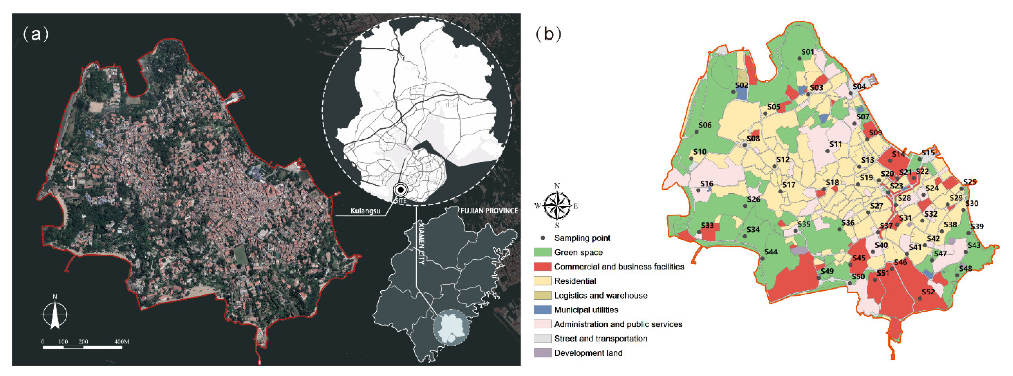
Figure 2.
Spatiotemporal distribution and temporal variation of the mean values of sound source dominance of the four main category sound sources.
Figure 2.
Spatiotemporal distribution and temporal variation of the mean values of sound source dominance of the four main category sound sources.
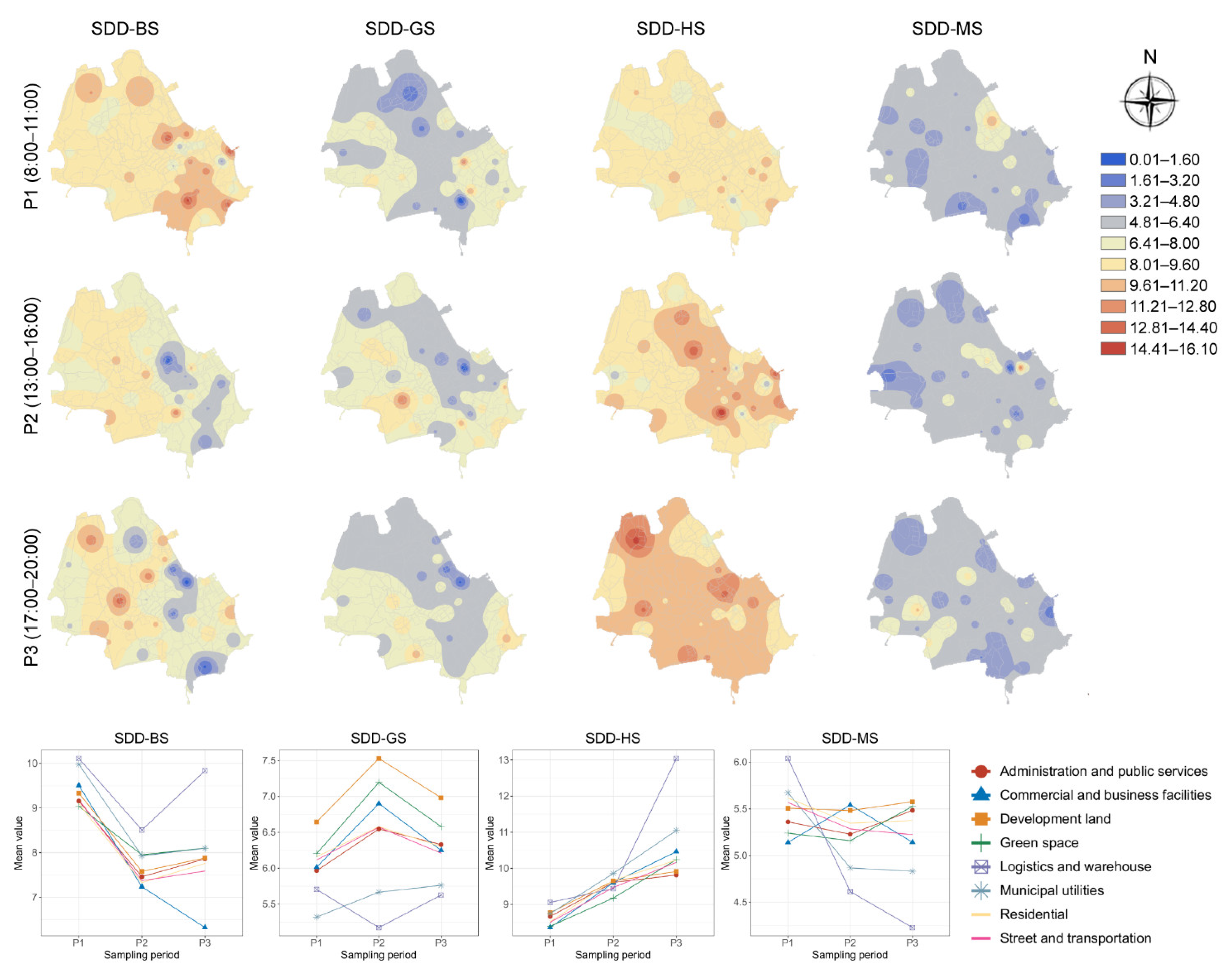
Figure 3.
Spatiotemporal distribution and temporal variation of the mean values of pleasantness and eventfulness.
Figure 3.
Spatiotemporal distribution and temporal variation of the mean values of pleasantness and eventfulness.
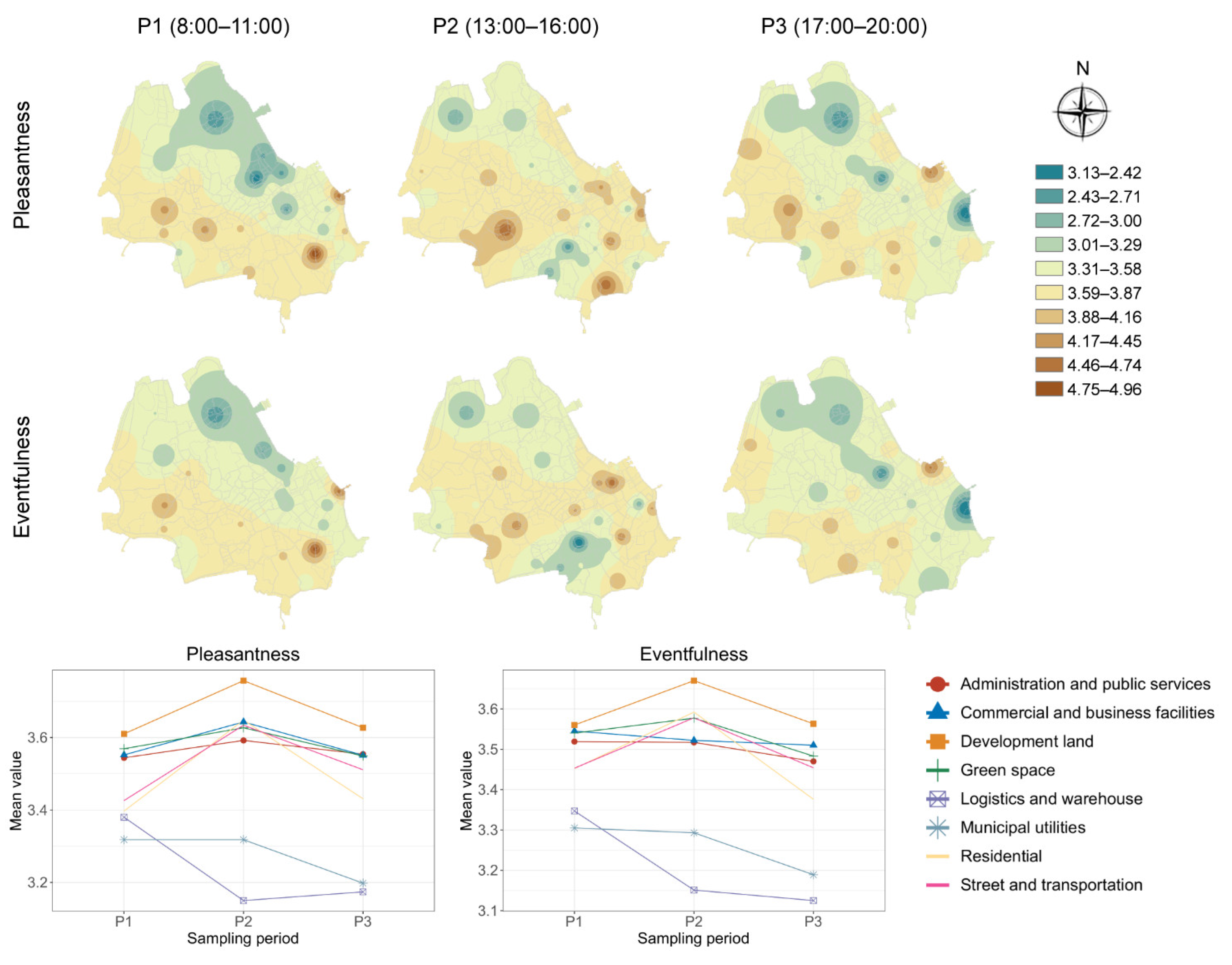
Figure 4.
Spatiotemporal variation and temporal variation of the mean values of landscape satisfaction degree.
Figure 4.
Spatiotemporal variation and temporal variation of the mean values of landscape satisfaction degree.
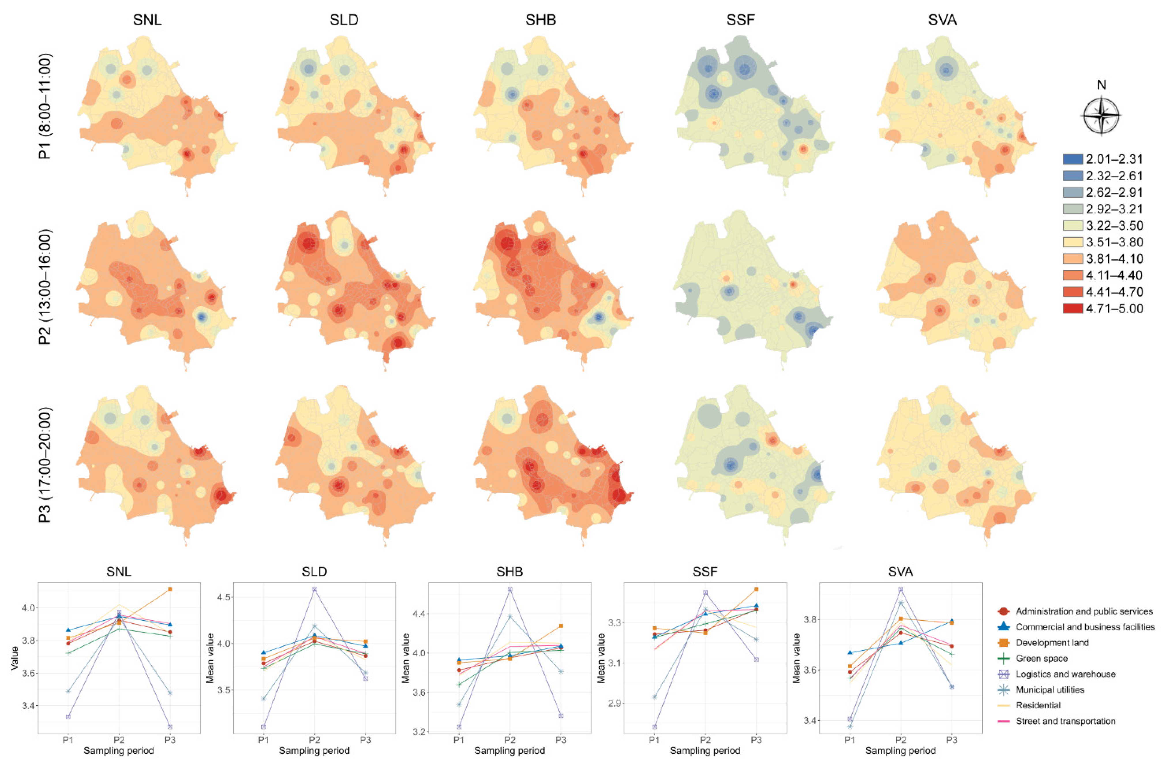
Figure 5.
The spatial features of green spaces: (a) distance to green spaces (DtGS) and (b) normalized difference vegetation index (NDVI).
Figure 5.
The spatial features of green spaces: (a) distance to green spaces (DtGS) and (b) normalized difference vegetation index (NDVI).
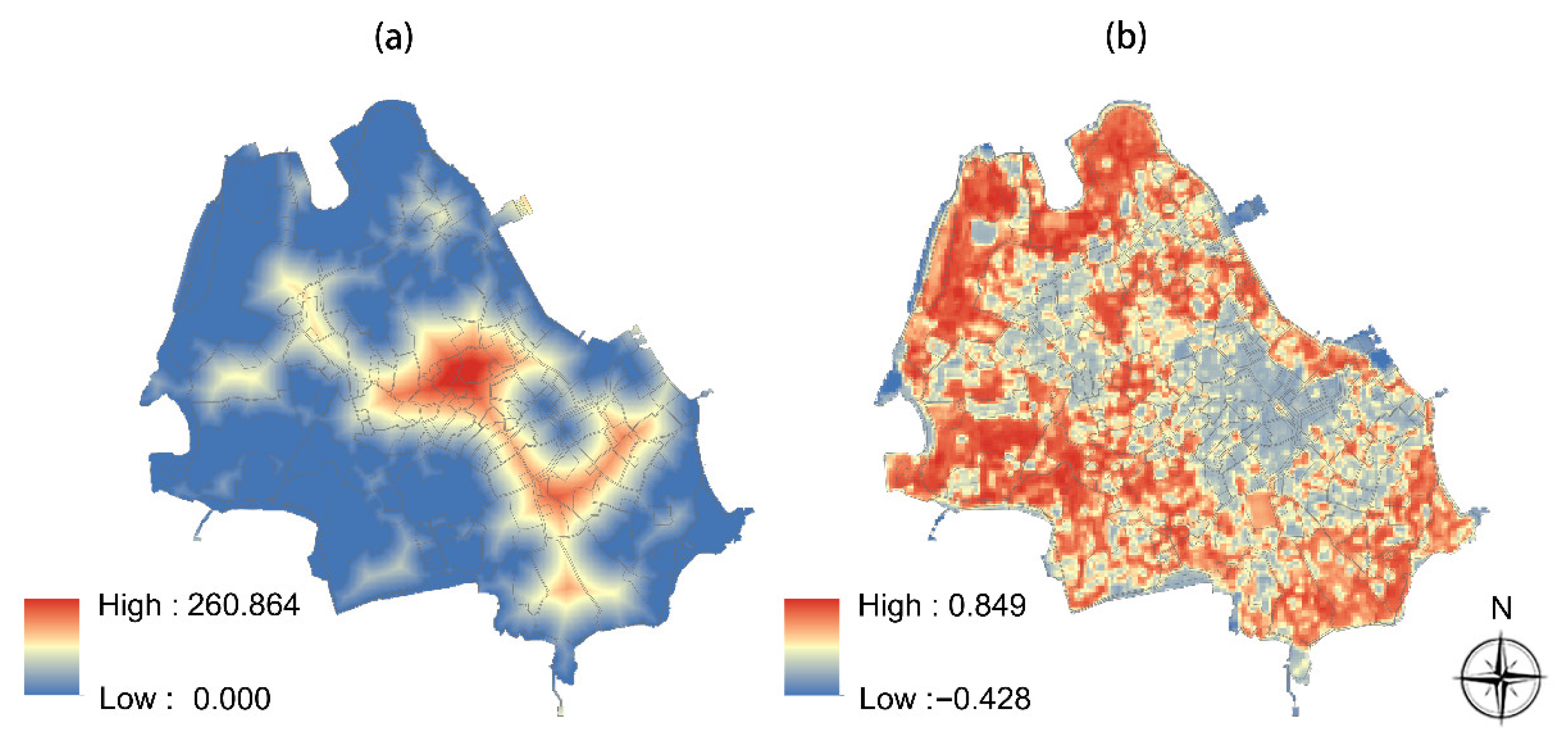
Figure 6.
Landscape spatial patterns in (a) class metrics and (b) landscape metrics.
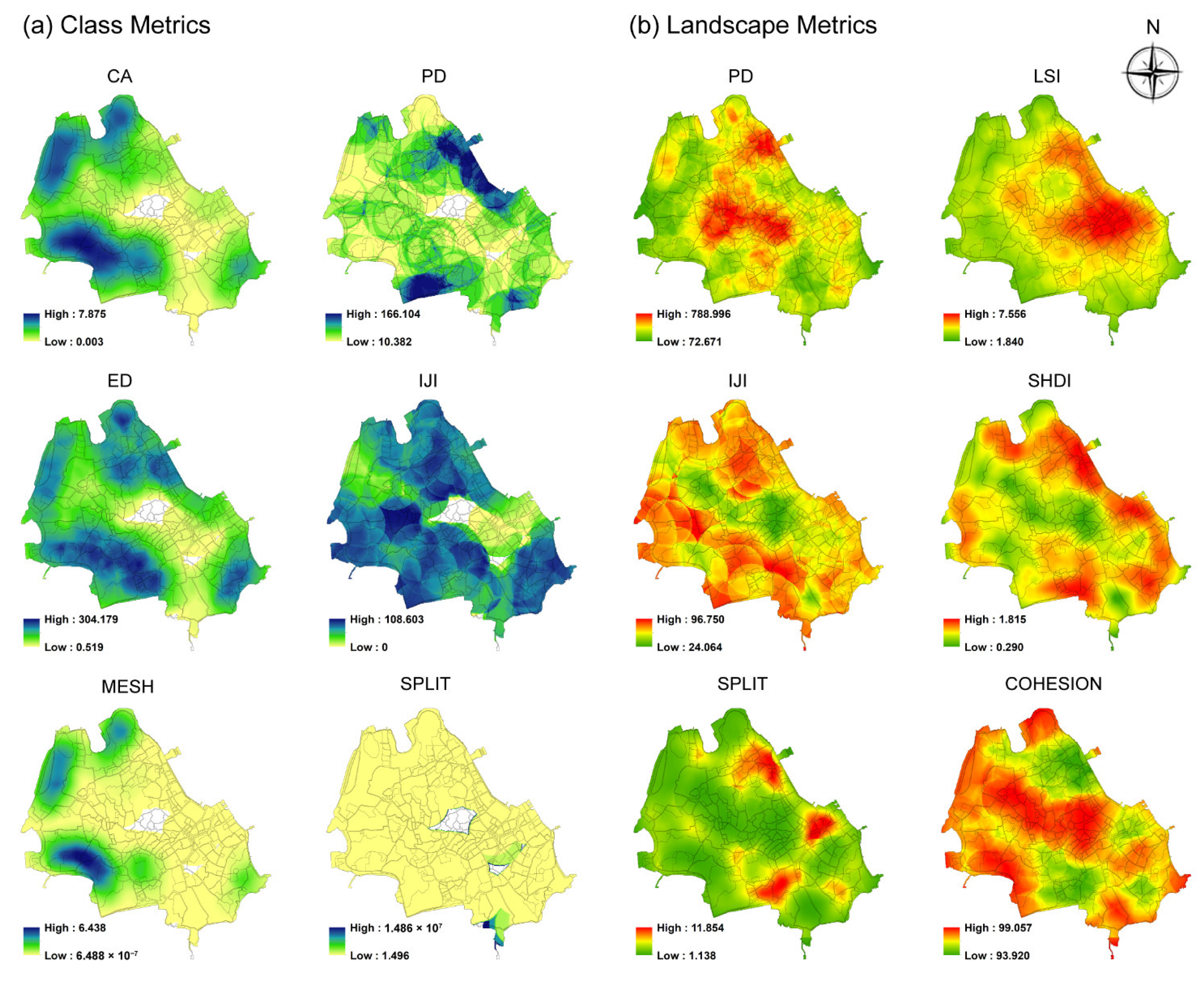
Figure 7.
Spatial distribution of local R2 for pleasantness and eventfulness in the three and total sampling periods.
Figure 7.
Spatial distribution of local R2 for pleasantness and eventfulness in the three and total sampling periods.
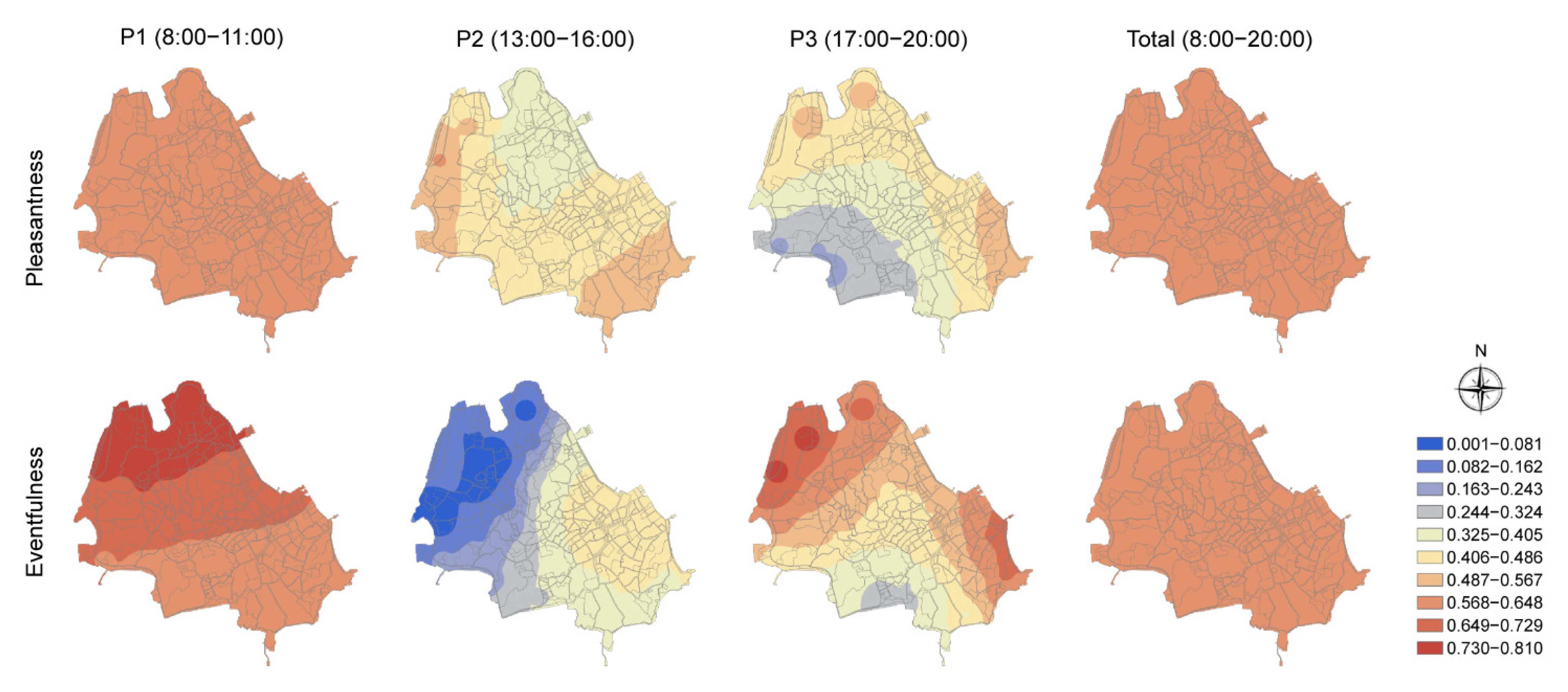
Figure 8.
Spatial distribution of local coefficients of significant variables in the three and total sampling period.
Figure 8.
Spatial distribution of local coefficients of significant variables in the three and total sampling period.

Table 1.
Classification of sound sources in the study area.
| Main Category (Abbreviation) | Sub-Category |
|---|---|
| Human activity sound (HS) | Talking, footstep, playing children, hawking, folk activity, live performance |
| Mechanical sound (MS) | Music radio, broadcast notification, construction, traffic noise, alarm |
| Biological sound (BS) | Birdsong, insect, cat |
| Geophysical sound (GS) | Sea wave, wind, tree, water, raining |
Table 2.
Detailed information for each perceived indicator.
| Category | Indicators (Abbreviation) | Survey Question | Rating Scale or Formula | Reference |
|---|---|---|---|---|
| Sound source | Perceived occurrences of sound (POS) | To what frequency do you presently hear the following four types of sounds? | 1-never, 2-occasionally, 3-normal, 4-frequently, 5-too frequently | [12,17,24] |
| Perceived loudness of sound (PLS) | To what intensity do you presently hear the following four types of sounds? | 1-too weak, 2-weak, 3-neither weak nor strong, 4-strong, 5-too strong | ||
| Sound dominant degree (SDD) | / | SDDij = POSij × PLSij | ||
| Soundscape quality | Pleasant | To what extent do you agree or disagree that the present surrounding sound environment is …? | 1-strongly disagree, 2-disagree, 3-general, 4-agree, 5-strongly agree | [37] |
| Comfort | ||||
| Harmonious | ||||
| Vivid | ||||
| Richness | ||||
| Eventful | ||||
| Landscape satisfaction degree | Satisfaction of natural landscapes (SNL) | To what extent do you satisfy or dissatisfy that the present surrounding landscape with regard to …? | 1-very dissatisfied, 2-not satisfied, 3-general, 4-satisfied, 5-very satisfied | [12,27] |
| Satisfaction of landscape design (SLD) | ||||
| Satisfaction of historical building (SHB) | ||||
| Satisfaction of visual-audio experience (SVA) | ||||
| Satisfaction of service facilities (SSF) |
Notes: j is the jth sample, i is the ith source, and n is the sample size.
Table 3.
Rotated component matrices of the PCA based on semantic attributes (numbers in parentheses represent explained variance).
Table 3.
Rotated component matrices of the PCA based on semantic attributes (numbers in parentheses represent explained variance).
| Semantic Attribute | Component 1: Pleasantness (41.8%) | Component 2: Eventfulness (38.8%) |
|---|---|---|
| Pleasant | 0.880 | 0.250 |
| Comfort | 0.906 | 0.236 |
| Harmony | 0.739 | 0.441 |
| Vivid | 0.491 | 0.703 |
| Richness | 0.295 | 0.867 |
| Eventful | 0.195 | 0.877 |
Table 4.
Results of the OLS model (* p < 0.05, ** p < 0.01).
| Sampling Period | Indicator | Pleasantness | Eventfulness | ||
|---|---|---|---|---|---|
| P1 | Independent variable | SDD-MS | −0.505 ** | SDD-BS | 0.170 * |
| SHB | 0.330 * | SDD-MS | −0.345 * | ||
| SVA | 0.312 ** | SVA | 0.407 ** | ||
| R2 | 0.653 | 0.591 | |||
| AIC | −59.061 | −56.234 | |||
| P2 | Independent variable | SDD-GS | 0.433 * | SLD | 0.295 ** |
| SLD | 0.362 ** | ||||
| R2 | 0.302 | 0.328 | |||
| AIC | −5.066 | −19.834 | |||
| P3 | Independent variable | SLD | 0.401 * | SLD | 0.497 ** |
| R2 | 0.379 | 0.418 | |||
| AIC | −17.154 | −31.585 | |||
| Total | Independent variable | SDD-BS | 0.196 ** | SDD-BS | 0.238 ** |
| SDD-GS | 0.299 ** | SDD-GS | 0.234 * | ||
| SLD | 0.510 ** | SLD | 0.504 ** | ||
| SSF | 0.351 * | ||||
| R2 | 0.649 | 0.591 | |||
| AIC | −62.988 | −50.111 | |||
Table 5.
R2 and AIC of the GWR model.
| Sampling Period | Indicator | Pleasantness | Eventfulness | |
|---|---|---|---|---|
| P1 | R2 | Mean | 0.596 | 0.674 |
| Minimum | 0.588 | 0.577 | ||
| Maximum | 0.645 | 0.81 | ||
| AIC | −69.975 | −84.445 | ||
| P2 | R2 | Mean | 0.507 | 0.380 |
| Minimum | 0.343 | 0.001 | ||
| Maximum | 0.58 | 0.453 | ||
| AIC | −46.329 | −46.172 | ||
| P3 | R2 | Mean | 0.468 | 0.601 |
| Minimum | 0.212 | 0.258 | ||
| Maximum | 0.558 | 0.773 | ||
| AIC | −51.287 | −75.251 | ||
| Total | R2 | Mean | 0.598 | 0.615 |
| Minimum | 0.62156 | 0.64534 | ||
| Maximum | 0.62183 | 0.64564 | ||
| AIC | −84.948 | −80.86 |
Note: To account for differences, the maximum and minimum values of the R2 of the GWR models for the total dataset were retained to five decimal places.
Publisher’s Note: MDPI stays neutral with regard to jurisdictional claims in published maps and institutional affiliations. |
© 2022 by the authors. Licensee MDPI, Basel, Switzerland. This article is an open access article distributed under the terms and conditions of the Creative Commons Attribution (CC BY) license (https://creativecommons.org/licenses/by/4.0/).
Share and Cite
MDPI and ACS Style
Chen, Z.; Zhu, T.-Y.; Liu, J.; Hong, X.-C. Before Becoming a World Heritage: Spatiotemporal Dynamics and Spatial Dependency of the Soundscapes in Kulangsu Scenic Area, China. Forests 2022, 13, 1526. https://doi.org/10.3390/f13091526
AMA Style
Chen Z, Zhu T-Y, Liu J, Hong X-C. Before Becoming a World Heritage: Spatiotemporal Dynamics and Spatial Dependency of the Soundscapes in Kulangsu Scenic Area, China. Forests. 2022; 13(9):1526. https://doi.org/10.3390/f13091526
Chicago/Turabian StyleChen, Zhu, Tian-Yuan Zhu, Jiang Liu, and Xin-Chen Hong. 2022. "Before Becoming a World Heritage: Spatiotemporal Dynamics and Spatial Dependency of the Soundscapes in Kulangsu Scenic Area, China" Forests 13, no. 9: 1526. https://doi.org/10.3390/f13091526
Note that from the first issue of 2016, this journal uses article numbers instead of page numbers. See further details here.