
Biomass Spatial Pattern and Driving Factors of Different Vegetation Types of Public Welfare Forests in Hunan Province

1
College of Biological Science and Technology, Central South University of Forestry and Technology, Changsha 410004, China
2
National Engineering Laboratory for Applied Forest Ecological Technology, Changsha 410004, China
3
College of Science, Central South University of Forestry and Technology, Changsha 410004, China
4
Hunan Jinghui Agroforestry Ecological Technology Co., Ltd., Changsha 410004, China
*
Author to whom correspondence should be addressed.
Forests 2023, 14(5), 1061; https://doi.org/10.3390/f14051061
Submission received: 6 April 2023
/
Revised: 12 May 2023
/
Accepted: 18 May 2023
/
Published: 22 May 2023
(This article belongs to the Section Forest Inventory, Modeling and Remote Sensing)
Abstract
:An ecological public welfare forest is an important basis for the construction of national ecological security. This study took public welfare forests at the provincial level or above in Hunan Province as the research object. Based on the in situ monitoring data and remote sensing data, we constructed a random forest (RF) model for inversing the biomass of public welfare forests with different types. Then, based on the inversion results, we investigated the biomass spatial pattern. Combined with topographical and socio-economic factors, we constructed a geographically weighted regression (GWR) model to analyze the biomass driving factors of different vegetation types in public forests. The results showed the following: (1) The biomass of public welfare forests in Hunan Province presented a strip distribution pattern that gradually increases from the central to the southwest and northeast. The total biomass of public welfare forests in Hunan Province was 338.13 million tons, with an average biomass of 68.31 t·hm−2. In the different types of public welfare forests, the mean biomass of the types were as follows: shrub (4.65 t·hm−2) < broadleaf forest (59.27 t·hm−2) < conifer–broadleaf mixed forest (62.44 t·hm−2) < bamboo forest (71.33 t·hm−2) < coniferous forest (100.33 t·hm−2). (2) Topographic and socio-economic factors have a significant impact on the spatial pattern of biomass in public welfare forests. Slope had the greatest effect on coniferous forest, conifer–broadleaf mixed forest, and shrub forest, while POP had the greatest effect on broadleaf forest and bamboo forest. This study investigates the spatial patterns and driving factors of biomass in public welfare forests at the provincial level, filling the gap in forest biomass monitoring in public welfare forests in Hunan Province. It provides a new method to improve the accuracy of forest biomass estimation and data support for the sustainable management of public welfare forests.
1. Introduction
The ecological public welfare forest is an important shelter forest that provides forestry ecology and social services, with the main functions of maintaining and improving the ecological environment, maintaining ecological balance, and protecting biodiversity. [1]. It is a critical foundation for the development of national ecological security [2]. However, most of the sites involved in the project are areas with poor soil conditions and those prone to water loss and soil erosion [3]. As a result, it is vital to clarify the spatial pattern of public welfare forests and investigate the driving causes in order to develop feasible policies for public welfare forest management, maintenance, and operations. In recent years, a large number of scholars have used remote sensing technology combined with biomass sampling plot surveys to estimate forest biomass in large regional scales [4,5]. Among them, Landsat series satellites have unique advantages. They can provide long-term, free to access historical archives with high spatial resolution. Therefore, they have become a main optical remote sensing data source for estimating forest biomass [6,7,8]. Machine learning has become popular in this century and has been widely used in remote sensing data processing. Nguyen et al. [9] compared 18 different models, and the results showed that RF was the model with the highest accuracy. López-Serrano et al. [10] used four machine learning methods to estimate the aboveground biomass of the temperate forests of the Durango State on the western Sierra Madre, NW Mexico, based on Landsat 8 OLI and forest resource fixed plot data. Jiang et al. [11] using spaceborne LiDAR and machine learning algorithms to improved aboveground biomass estimation of natural forests on the Tibetan Plateau, and the results show that the optimized extreme learning machine (ELM) achieved the best estimation effect among all the analyzed models. Among a variety of methods for biomass estimation, RF modeling was found to have the great advantages of high estimation accuracy and operability. Forest biomass is affected by a variety of driving factors. Topographic factors, including elevation, slope, and aspect, had been widely considered to be the main factors affecting the spatial pattern of forest biomass [12,13]. Socio-economic drivers, including gross domestic product (GDP) and population (POP), also play an irreplaceable role [14]. Alves et al. [15] studied the aboveground biomass and forest structure on the elevation gradient in the humid zone of the tropical Atlantic in Brazil, and it was found that the distribution of aboveground biomass was affected by the local scale topographic changes related to elevation. Li et al. [12] analyzed the dynamics and driving factors of mountain forest biomass in Southwest China from 1979 to 2017, and concluded that climate change has a negative impact on forest biomass and that policy adjustments help maintain forest biomass in Southwest China. The geographically weighted regression (GWR) model can fully indicate the characteristics of spatial structure heterogeneity, revealing the underlying driving factors more effectively [16,17].
After 20 years’ protection, as one of the first 11 pilot provinces in China to protect public welfare forests, Hunan Province has constructed ecological public welfare forests with stable structure and complete functions. Currently, there is a lack of an overall evaluation of the public welfare forests in Hunan Province, as well as a limited understanding of the spatial pattern and driving factors of forest biomass. Therefore, the objectives of this study are as follows: (1) extract modeling variables from Landsat 8 remote sensing imagery using the Boruta algorithm for feature selection and construct biomass inversion models for different types of public forests using the RF method; (2) inverse the biomass spatial pattern in public welfare forests according to inversion results; (3) apply the ordinary least square (OLS) method to select factors, and construct the GWR model to analyze the driving factors of biomass in different types of public welfare forests; and (4) provide management and sustainable operating strategies for different types of public welfare forests.
2. Materials and Methods
2.1. Study Area
The study area is located in Hunan Province (108°47’–114°15’ E, 24°38’–30°08’ N) in the middle and upper reaches of the Yangtze River and south of Dongting Lake, which belongs to the subtropical monsoon humid climate (Figure 1). The topography of Hunan Province presents an asymmetric “U-shaped” form surrounded by mountains in the east, west, and south, gradually tilting towards the center and northeast. According to the “one map” of forest resource management in Hunan Province in 2021, the total area of public welfare forests at the provincial level or above (hereinafter referred to as “public welfare forests”) in Hunan Province is 4.95 hm2, accounting for 23.36% of the provincial land area. According to the China Vegetation Zoning and the criteria for forest community characteristics, the public welfare forests in Hunan Province can be roughly divided into five vegetation types, including coniferous forest, broadleaf forest, conifer–broadleaf mixed forest, bamboo forest, and shrub (Table 1, Figure 1b).
2.2. Data Collection
2.2.1. In Situ Monitoring Data
This study used in situ monitoring data from 682 sampling plots of public welfare forests in Hunan Province in 2021 (Figure 1b). The survey plots were rectangular in shape, measuring 25 m by 40 m, with a total area of 1000 m2. The monitoring data included a series of attributes, such as plot code, coordinates, vegetation type, dominant tree species, diameter at breast height (DBH), and tree height. The biomass of each individual tree in the sample plot was then calculated based on 28 biomass equations for major species in Hunan [18], as well as for individual bamboo plants [19] and groups of broadleaf trees categorized as fast-growing, medium-growing, and slow-growing [20]. The biomass of each sample plot was calculated by aggregating the biomass of each tree within the plot. According to the classification of vegetation types, the sample plots were classified into five vegetation types, and the statistical results of the biomass of the plots are shown in Table 2.
2.2.2. Remote Sensing Data
This study used the Landsat 8 landmark reflectance product (LANDSAT/LC08/C01/T1_SR) with 30 m spatial resolution provided by the Google Earth Engine (GEE) platform. In total, 266 images with cloud cover less than 5% were selected from May to October of 2021, which covered the whole period of the ground survey. In addition, the CFMask algorithm was used to mask pixels covered by clouds, shadows, water, and snow. Mosaic and clip functions were performed to fuse, splice, and clip the images that could represent the best vegetation growth state in the study area. In ENVI 5.3, 115 remote sensing spectral variables in 5 categories were extracted, including original band, band combinations, image transformations, vegetation indices, and texture measures, as alternative parameters for construct the model (Table 3).
2.2.3. Driving Factor Data
This paper selected three topographic factors, namely elevation, slope, and aspect, two socio-economic factors, POP and GDP, and two climatic factors, annual average temperature and annual average precipitation, to investigate the impact of seven factors on the spatial variation of biomass in public forests in Hunan Province (Table 4). The digital elevation model (DEM) with spatial resolution of 30 m by 30 m was downloaded from the Geospatial Data Cloud (http://www.gscloud.cn/, accessed on 10 February 2022) for the extraction of elevation, slope, and aspect. The 2020 GDP and POP data provided by the Resources and Environment Science and Data Center, Chinese Academy of Sciences (http://www.resdc.cn/DOI, accessed on 12 February 2022), were used to replace the traditional administrative statistics unit with the spatial statistical unit to realize the spatialization of GDP and POP [21,22]. In addition, climate data were from National Tibetan Plateau Data Center (http://data.tpdc.ac.cn/zh-hans/, accessed on 15 February 2022), including the 1 km monthly mean temperature dataset for China (1901–2021) [23] and 1 km monthly precipitation dataset for China (1901–2021) [24].
2.3. Methods
2.3.1. Methods of Variable Selection
Boruta Algorithm
The Boruta algorithm is a feature selection algorithm based on RF. Firstly, the original feature dataset is rearranged to create mixed copies and generate shadow features. Secondly, the importance of the shadow feature set is sorted according to the precision discrimination index of RF. The importance scores of variables in the original feature set are observed through several iterations, and the importance of variables with low importance is gradually eliminated by comparing their importance. Finally, all variable characteristics are confirmed or removed. The Boruta algorithm was executed in PyCharm software (Community 2022.1.1; JetBrains PyCharm, Prague, Czech Republic).
Ordinary Least Square Method
The ordinary least square method (OLS) extracts comprehensive variables with strong explanatory power to dependent variables through spatial transformation of the independent variable, making the estimated value more precise. The model calculation formula is as follows:
where is the dependent variable, is the regression intercept, represents each explanatory variable, represents the regression coefficient of the kth explanatory variable to the explained variable , and represents the random error term.
2.3.2. Random Forest
RF is one of the most commonly used classification and regression algorithms to explain the complex relationship between dependent variables and multiple independent variables [25]. It relies on random selection of samples and features to eliminate overfitting problems. In order to make full use of the samples to improve the reliability of the model, the study divided the dataset with 70% data as training data and 30% data as validation data in the PyCharm software(Community 2022.1.1; JetBrains PyCharm, Prague, Czech Republic).
2.3.3. Geographically Weighted Regression
Geographically weighted regression (GWR) is a spatial statistical model used to explore spatial changes and driving factors of spatial objects at a certain dimension. GWR detects the non-stationarity of spatial relations by embedding spatial structure into the linear regression model. Its mathematical model form is shown in Formula (2):
where is the dependent variable at location i, is the intercept coefficient, is the kth explanatory variable, is the local regression coefficient for the kth explanatory variable, and is the random error term. The GWR model was computed in ArcGIS 10.8(Esri ArcGIS, Redlands, CA, USA), and the regression coefficients and intercepts of each grid reflect the degree of spatial variation in the influence of independent variables on the dependent variable.
2.3.4. Evaluation Metrics
The coefficient of determination (R2) [26] and the root-mean-square error (RMSE) [26] were used to evaluate the performance of the final models:
where is the observed biomass value, is the predicted biomass value based on models, is the arithmetic mean of all the observed biomass values, and is the sample number. In general, a higher value and lower values indicate a better estimation performance of the model.
3. Results
3.1. Results of Biomass Inversion of Public Welfare Forest
In this study, we used the measured biomass data of different types of public forests as the dependent variable and 115 remote sensing factors as independent variables. The important characteristic variables related to biomass of each vegetation category were selected by Boruta algorithm and shown in Table 5.
According to the predicted results of the biomass inversion model (Figure 2), bamboo forest presented the highest accuracy (RMSE = 26.50 t·hm−2, R2 = 0.79), followed by conifer–broadleaf mixed forest (RMSE = 15.76 t·hm −2, R2 = 0.76), coniferous forest (RMSE = 31.76 t·hm−2, R2 = 0.74), shrub (RMSE = 2.11 t·hm−2, R2 = 0.74), and broadleaf forest (RMSE = 21.57 t·hm−2, R2 = 0.73), with total forest (RMSE = 30.77 t·hm−2, R2 = 0.67) being the lowest.
3.2. Spatial Pattern of Biomass of Public Welfare Forest
Classification of forest types can improve the generalization performance and accuracy of the model. Therefore, according to the forest type, the RF model was used to generate the corresponding biomass spatial distribution map (Figure 3). Furthermore, the total biomass map of public welfare forests in Hunan Province was also generated by combining the spatial distribution maps of different types of biomass (Figure 3f). It can be observed that the mean biomass of public welfare forests in Hunan Province was 68.15 t·hm−2, and the total biomass was 338.15 million tons. Spatially, the biomass of public welfare forests in Hunan Province ranged from 0.85 to 177.63 t·hm−2, showing a strip distribution pattern that gradually increases from the central to the southwest and northeast. The areas with high biomass (>75 t·hm−2) in the public welfare forests were mainly concentrated in the southeastern Luoxiao Mountain range, southern Nanling Mountain range, southwestern Wuling Mountain range, and Xuefeng Mountain range, where there were more natural reserves, forest parks, and less human disturbance. Instead, the low-biomass (<30 t·hm−2) areas were mainly located in the valley plain of the Xiangjiang River Basin and the central Hunan Hill, in which shrubs were mainly distributed.
In various types of public welfare forests, the mean biomass in ascending order were as follows: shrub (4.65 t·hm−2) < broadleaf forest (59.27 t·hm−2) < conifer–broadleaf mixed forest (62.44 t·hm−2) < bamboo forest (71.33 t·hm−2) < coniferous forest (100.33 t·hm−2). The total biomass in ascending order were as follows: shrub forest (4.33 million tons) < bamboo forest (33.32 million tons) < conifer–broadleaf mixed forest (36.97 million tons) < broadleaf forest (48.45 million tons) < coniferous forest (215.24 million tons). The biomass of different types of public welfare forest were correlated with the forest area and the mean biomass (Figure 4). Coniferous forest had the largest distribution area and the highest mean biomass, and its contribution accounted for 63.64% of the total public welfare forest biomass. The shrub forest had a large area, though its mean biomass was the smallest, and thus it contributed the least biomass (1.28%) to the total public welfare forest (Table 6).
3.3. Analysis of Results of Geographically Weighted Regression Model
The OLS was used in this study to select driving factors. According to the selection results (Table 7), the accuracy R2 of the biomass models of coniferous forest, broadleaf forest, conifer–broadleaf mixed forest, bamboo forest, and shrub were 0.47, 0.43, 0.52, 0.47, and 0.56, and the AICc values were 165,941.69, 59,308.81, 38,989. 15, 31,852.20, and 33,110. 13, respectively. The t and p values of each driving factor were statistically significant, and the VIFs were all less than 10. For this reason, it can be seen that there is no collinearity problem between the selected driving factors, and they can be used to construct the GWR model.
The spatial distribution of the factor regression coefficient and intercept of the GWR models of biomass of different types were compared and analyzed (Table 8). The results showed that each factor explained 29%, 27%, 39%, 41%, and 48% of the spatial variation of the biomass of coniferous forest, broadleaf forest, conifer–broadleaf mixed forest, bamboo forest, and shrub, respectively. According to the absolute value of the median regression coefficients of each driving factor in the GWR, the contribution of each driving factor to forest biomass was ranked as follows: coniferous forest, slope > aspect > GDP > elevation > POP; broadleaf forest, POP > elevation > GDP; conifer–broadleaf mixed forest, slope > POP > GDP > elevation > aspect; bamboo forest, POP > elevation > GDP; and shrub, slope > GDP > POP > aspect. The biomass of different types have different correlations with various driving factors. In the coniferous forest, GDP and POP were negatively correlated with biomass, while elevation, slope, and aspect were positively correlated with biomass distribution. For the broadleaf forest, POP and biomass were significantly negatively correlated, while elevation, GDP, and biomass were slightly positively correlated. For the broadleaf mixed forest, slope, GDP, and biomass were significantly negatively correlated, while elevation, aspect, and POP were positively correlated with biomass. For the bamboo forest, GDP and POP were significantly negatively correlated with biomass, while elevation and biomass were significantly positively correlated. For shrubs, GDP and POP were significantly negatively correlated with biomass, and slope and aspect were significantly positively correlated with biomass.
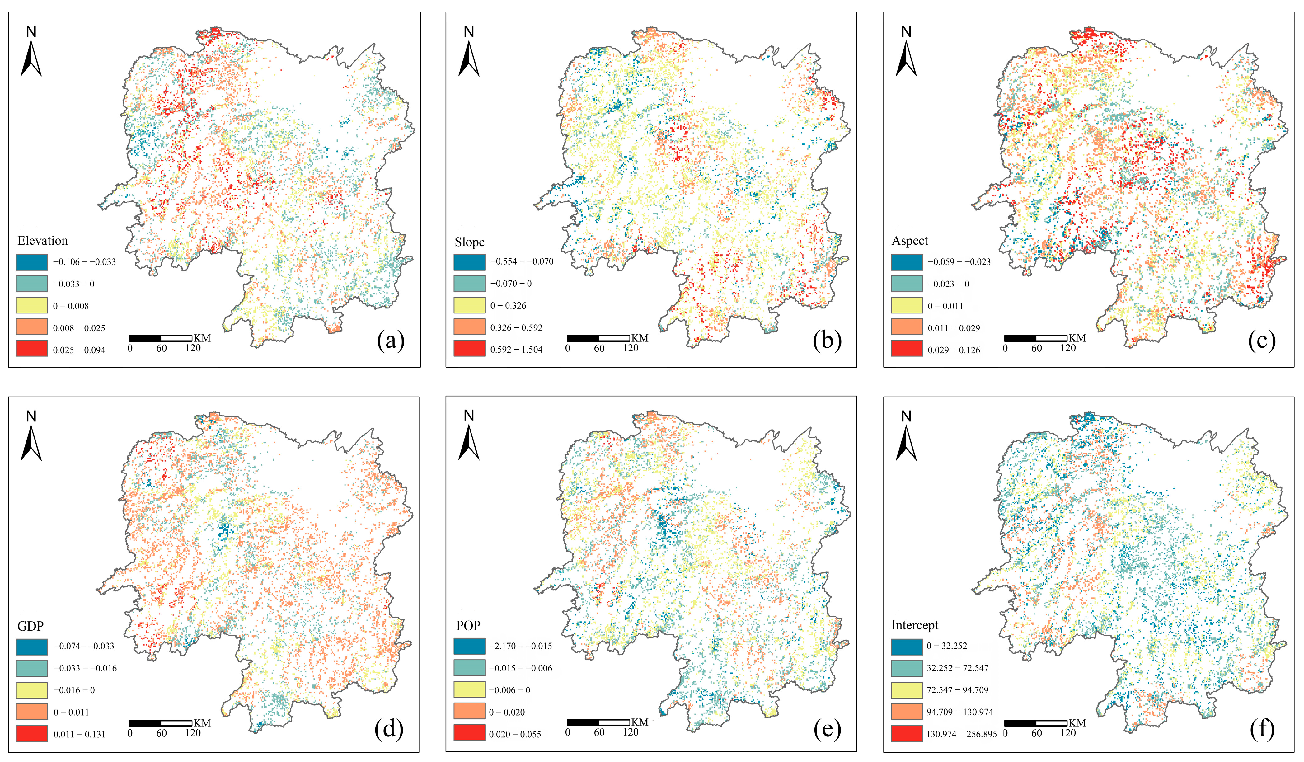
The GWR coefficients and intercepts of different types of public welfare forest biomass in Hunan Province were integrated into the spatial distribution of the total forest (Table 9, Figure 5). The contribution of each driving factor to the biomass of public welfare forests in Hunan Province was ranked as follows: slope > GDP > aspect > POP > elevation. Elevation, slope, and aspect had significant positive effects on biomass distribution, among which the positive effect of elevation on biomass of public welfare forests (regression coefficient > 0) was larger in area, accounting for 62.51% of the total area, which was mainly distributed in the Huping Mountains, Wuling Mountains, and Xuefeng Mountains in the western part of the study area. GDP and POP had significant negative effects on biomass distribution, and the areas with negative effects were mainly the Wanyang Mountains and low-elevation hills in central Hunan.
4. Discussion
4.1. Biomass of Different Types of Forests
We compared the field survey values of public welfare forest biomass with that from model estimations for different vegetation types. The data are generally reliable. In particular, there is a phenomenon of high-value underestimation and low-value overestimation. For example, the coniferous forest field survey data were 107.67 t·hm−2, and the model estimated value was 100.33 t·hm−2. The bias could result from the uncertainty of remote sensing data used on the study area, or the uneven distribution of sample points.
According to the biomass estimation results of different vegetation types of public welfare forests, the mean biomass of the coniferous forest (100.33 t·hm−2) was significantly higher than that of other types. The main reason may be that other forests were young and middle-aged, while the coniferous forest was mature. The lowest mean biomass was found in the shrub forest (4.65 t·hm−2), and the main reasons leading to the low biomass may be the low crown height and small ground diameter and crown diameter of the shrubs [27]. Another potentially influential factor was the significant difference in the average environment of forests. With some exceptions, the shrub forest was mainly found in plain areas with elevation, flat terrain, and high human disturbance. The coniferous forest was found in mountainous areas with higher elevations, steeper terrain, and less anthropogenic influence. For other types of public welfare forests, it is expected that future biomass will continue to increase, and effective manual intervention will contribute more in Hunan Province [28].
4.2. Explanatory Power of Driving Factors
Many studies have proved that temperature can change the forest vegetation productivity and biomass by affecting plant photosynthesis and respiration [29]. Precipitation is an important way for plants to obtain water, which can affect the growth and development of plants, community characteristics, and ecosystem structure, thereby affecting the allocation of forest biomass. Sun et al. [30] concluded that there was a significant correlation between the biomass of broadleaf forests and climatic factors, such as maximum precipitation and maximum average temperature. Many scholars have also obtained the relationship between temperature and precipitation in their research objects based on specific tree species. In this study, when the biomass driving factors of various vegetation types were screened, precipitation and air temperature were not selected as two climate factors, which may be due to the fact that the impacts of climate change are complex [31], and forest biomass is regulated by the complex interaction among climate, topography, and socio-economic variables [32,33].
There are many factors affecting the spatial pattern of forest biomass, and topography is one of the most important ones [34]. The results of this study showed that topography factors had a positive effect on forest biomass, among which slope is the most influential. This may be because of the mountains and hills of the relatively rugged surface form in Hunan Province. With the increase in slope, the chance and degree of the forest being disturbed by human beings decreased and the vegetation biomass increased [35]. Moreover, aspect mainly influences solar radiation, which can affect the site growth of trees and can thus affect the biomass. For instance, the shrub forest was beneficial to growth on low-elevation and sunny, dry slopes [36]. Elevation controls the gradient changes in local temperature and precipitation through the evapotranspiration rate, and directly or indirectly affects forest biomass [37]. In general, without considering the management of the forest stands, the higher the elevation and the greater the slope, the less the stand was subjected to human disturbance, thus the greater the biomass accumulation. The water and heat conditions of aspects are different, which restrict the growth of trees and thus affect the biomass [38]. In this case, bamboo and broadleaf vegetation may be more suitable for the growth of light, water, temperature, and other conditions on sunny slopes.
The spatial pattern of forest biomass was affected by socio-economic factors. To be concrete, GDP and POP had strong negative effects on the biomass of forests. In 2021, the study area was in the stage of stable economic growth, and the quality of public welfare forests was greatly improved due to the policies of returning of farmland to forest, the construction of beautiful countryside, and the ecological compensation of public welfare forests. In the relatively developed economic period, the positive effect of economic construction on forest biomass was dominant. According to the environmental Kuznets curve, the relationship between forest carbon sink and per capita GDP presents a “U-shaped” curve [39]; POP has a gradually enhanced negative effect on the change in forest biomass, and the increase in population will inevitably lead to the increase in forest resource demand [40], which is consistent with our study. In recent years, large-scale human activities have had an important impact on the local environment. For example, Hunan Province has built in the ecological “green-core” area of the Changzhutan urban cluster. This “green-core” area has invested a large amount of funding to improve the quality and stability of the provincial ecosystem by focusing on the systematic management and improvement of mountains, rivers, forests, fields, lakes, and grasslands.
4.3. Biomass of Different Types of Public Welfare Forests Are Affected by Driving Factors
For the coniferous forest, the effect of topography on biomass was significantly greater than that of other factors. This may be due to the fact that the vegetation roots of the coniferous forest were well developed and more restricted by topography. For example, the areas affected by elevation with a large coniferous forest coefficient were concentrated in the mountain areas, such as the Wuling Mountains and Xuefeng Mountains in western Hunan Province, which had a large relief amplitude and little human disturbance, resulting in the larger biomass.
The biomass of the broadleaf forest was negatively affected by POP. The distribution area of the broadleaf forest was mainly in the middle and low latitudes, which tended to have higher population density and rapid economic development. Accordingly, the demand and pressure on forest resources were also greater. The increase in population also meant that more lands were reclaimed, felled, and used for agricultural production, which had a negative impact on broadleaf forest biomass. The impact was not only exerted on the broadleaf forest, but also on other forests.
The conifer–broadleaf mixed forest was distributed in open plains and mountain areas at lower elevations. It was composed of a variety of tree species mixed with each other and had higher species diversity and structural complexity. Slope then affected the uncertainty of tree species to a certain extent, and its influence on richness was greater than evenness [41].
There was an obvious negative correlation between bamboo biomass and elevation. Moso bamboo (Phyllostachys edulis) is the main dominant species of bamboo forests whose early and late dates of bamboo shoot growth mainly depend on the continuous temperature in a period before that. Elevation, then, was the main factor affecting temperature and humidity. Studies have shown that the biomass of bamboo forests presented an overall increasing trend first, and then a decreasing trend with the increase in elevation, and both high and low elevation were not conducive to the growth of bamboo [42]. To cultivate high-yield and high-quality bamboo forests, the elevation should be below 800 m [43].
The fact that the shrub forest was more affected by slope, but not by elevation, was related to its adaptation to the environment. On the one hand, shrub roots are not more adaptable than tress. Shrubs need stronger adaptability to maintain their growth. On the other hand, the change in slope will lead to the change in temperature, light, and oxygen concentration, which will affect the growth and development of shrubs.
5. Conclusions
This study focused on the public forests of different vegetation types (coniferous forest, broadleaf forest, conifer–broadleaf mixed forest, bamboo forest, and shrub) in Hunan Province. The Boruta algorithm was used to screen the Landsat 8 OLI modeling variables, and an RF model was constructed for the biomass of public forests of different vegetation types, exploring their spatial patterns. Combined with topographic, socio-economic, and other factors, seven driving factors were screened by the OLS model to construct a different vegetation type biomass GWR model, which identified the driving factors of biomass in public forests with different vegetation types. The results showed that in 2021, the biomass of public welfare forests in Hunan Province presented a strip distribution pattern that gradually increased from the central to the southwest and northeast. The total biomass of public welfare forests in Hunan Province was 338.13 million tons, with an average biomass of 68.31 t·hm−2. In the different types of public welfare forests, the mean biomass of each type was found: shrub (4.65 t·hm−2) < broadleaf forest (59.27 t·hm−2) < conifer–broadleaf mixed forest (62.44 t·hm−2) < bamboo forest (71.33 t·hm−2) < coniferous forest (100.33 t·hm−2). Topographic and socio-economic factors have significant impacts on the spatial pattern of biomass in ecological public forests. Slope had the greatest effect on coniferous forest, conifer–broadleaf mixed forest, and shrub, while POP had the greatest effect on broadleaf forest and bamboo forest.
This study investigates the spatial patterns and driving factors of biomass in public forests at the provincial level, filling the gap in forest biomass monitoring in public forests in Hunan Province. In view of the differences in mean biomass size, spatial pattern, and the main driving factors of different vegetation types of public welfare forests, we will subsequently research corresponding management measures and strategies for different types of public forests in Hunan Province to enhance the management quality and ecological service functions of public forests.
Author Contributions
Data curation: H.L., Y.F. and J.P.; formal analysis: H.L. and J.P.; funding acquisition: G.W.; methodology: H.L. and J.P.; project administration: G.W.; resources: G.W.; software: H.L.; supervision: G.W.; validation: H.L., Y.F. and K.H.; visualization: H.L. and J.P.; writing—original draft: H.L.; writing—review and editing: H.L., Y.F., J.P. and K.H. All authors have read and agreed to the published version of the manuscript.
Funding
This research is supported by the Key Research and Development Project of Hunan Province of China (Grant No. 2021Nk2018) and the Key Projects of Science and Technology of Guangxi Province of China (Grant No. AB21220026).
Data Availability Statement
Not applicable.
Acknowledgments
Meteorological datasets are provided by the National Tibetan Plateau Data Center (http://data.tpdc.ac.cn, accessed on 15 February 2022). Socio-economic datasets are provided by the Resource and Environmental Science and Data Center, Chinese Academy of Sciences (http://www.resdc.cn/DOI, accessed on 12 February 2022).
Conflicts of Interest
The authors declare no conflict of interest.
References
- Aguilar, F.X.; Wen, Y. Socio-economic and ecological impacts of China’s forest sector policies. For. Policy Econ. 2021, 127, 102454. [Google Scholar] [CrossRef]
- Zhang, B.; Li, W.; Xie, G. Ecosystem services research in China: Progress and perspective. Ecol. Econ. 2010, 69, 1389–1395. [Google Scholar] [CrossRef]
- Wenhua, L. Degradation and restoration of forest ecosystems in China. For. Ecol. Manag. 2004, 201, 33–41. [Google Scholar] [CrossRef]
- Halme, E.; Pellikka, P.; Mottus, M. Utility of hyperspectral compared to multispectral remote sensing data in estimating forest biomass and structure variables in Finnish boreal forest. Int. J. Appl. Earth Obs. Geoinf. 2019, 83, 101942. [Google Scholar] [CrossRef]
- Zhang, R.; Zhou, X.; Ouyang, Z.; Avitabile, V.; Qi, J.; Chen, J.; Giannico, V. Estimating aboveground biomass in subtropical forests of China by integrating multisource remote sensing and ground data. Remote Sens. Environ. 2019, 232, 111341. [Google Scholar] [CrossRef]
- Wulder, M.A.; Loveland, T.R.; Roy, D.P.; Crawford, C.J.; Masek, J.G.; Woodcock, C.E.; Allen, R.G.; Anderson, M.C.; Belward, A.S.; Cohen, W.B. Current status of Landsat program, science, and applications. Remote Sens. Environ. 2019, 225, 127–147. [Google Scholar] [CrossRef]
- Zhu, Z.; Wulder, M.A.; Roy, D.P.; Woodcock, C.E.; Hansen, M.C.; Radeloff, V.C.; Healey, S.P.; Schaaf, C.; Hostert, P.; Strobl, P. Benefits of the free and open Landsat data policy. Remote Sens. Environ. 2019, 224, 382–385. [Google Scholar] [CrossRef]
- Wulder, M.A.; Roy, D.P.; Radeloff, V.C.; Loveland, T.R.; Anderson, M.C.; Johnson, D.M.; Healey, S.; Zhu, Z.; Scambos, T.A.; Pahlevan, N. Fifty years of Landsat science and impacts. Remote Sens. Environ. 2022, 280, 113195. [Google Scholar] [CrossRef]
- Nguyen, T.H.; Jones, S.; Soto-Berelov, M.; Haywood, A.; Hislop, S. A comparison of imputation approaches for estimating forest biomass using Landsat time-series and inventory data. Remote Sens. 2018, 10, 1825. [Google Scholar] [CrossRef]
- López-Serrano, P.M.; Cárdenas Domínguez, J.L.; Corral-Rivas, J.J.; Jiménez, E.; López-Sánchez, C.A.; Vega-Nieva, D.J. Modeling of aboveground biomass with Landsat 8 OLI and machine learning in temperate forests. Forests 2019, 11, 11. [Google Scholar] [CrossRef]
- Jiang, F.; Sun, H.; Ma, K.; Fu, L.; Tang, J. Improving aboveground biomass estimation of natural forests on the Tibetan Plateau using spaceborne LiDAR and machine learning algorithms. Ecol. Indic. 2022, 143, 109365. [Google Scholar] [CrossRef]
- Li, T.; Zou, Y.; Liu, Y.; Luo, P.; Xiong, Q.; Lu, H.; Lai, C.; Axmacher, J.C. Mountain forest biomass dynamics and its drivers in southwestern China between 1979 and 2017. Ecol. Indic. 2022, 142, 109289. [Google Scholar] [CrossRef]
- Renner, M.; Rembold, K.; Hemp, A.; Fischer, M. Natural regeneration of woody plant species along an elevational and disturbance gradient at Mt. Kilimanjaro. For. Ecol. Manag. 2022, 520, 120404. [Google Scholar] [CrossRef]
- Kucuker, D.M.; Tuyoglu, O. Spatiotemporal patterns and driving factors of carbon dynamics in forest ecosystems: A case study from Turkey. Integr. Environ. Assess. Manag. 2022, 18, 209–223. [Google Scholar] [CrossRef] [PubMed]
- Alves, L.F.; Vieira, S.A.; Scaranello, M.A.; Camargo, P.B.; Santos, F.A.M.; Joly, C.A.; Martinelli, L.A. Forest structure and live aboveground biomass variation along an elevational gradient of tropical Atlantic moist forest (Brazil). For. Ecol. Manag. 2010, 260, 679–691. [Google Scholar] [CrossRef]
- Yu, S.; Ye, Q.; Zhao, Q.; Li, Z.; Zhang, M.; Zhu, H.; Zhao, Z. Effects of Driving Factors on Forest Aboveground Biomass (AGB) in China’s Loess Plateau by Using Spatial Regression Models. Remote Sens. 2022, 14, 2842. [Google Scholar] [CrossRef]
- Park, J.; Lim, B.; Lee, J. Analysis of Factors Influencing Forest Loss in South Korea: Statistical Models and Machine-Learning Model. Forests 2021, 12, 1636. [Google Scholar] [CrossRef]
- Luo, J.; Dai, C.D.; Tian, Y.X.; Peng, P.; Ma, F.F.; Zeng, Z.Q.; Zhou, X.L.; Zhang, M. Establishment of main constructive species biomass model for project forests of carbon sink in Hunan. Hunan For. Sci. Technol. 2016, 43, 12–16+21. [Google Scholar]
- Zeng, Z.Q.; Tian, Y.X.; Dai, C.D.; Peng, P.; Meng, Y.; Huang, Z.R.; Ye, C.J.; Ma, F.F.; Luo, J. Study on biomass model of Phyllostachys heterocycla cv pubescens in Hunan Province. Hunan For. Sci. Technol. 2016, 43, 56–59. [Google Scholar]
- Ma, F.F.; Wu, X.L.; Dai, C.D.; Peng, P.; Tian, Y.X.; Zeng, Z.Q. Construction of individual tree growth model of fast-growing, intermediate and slow growing broadleaf forest in Hunan. Hunan For. Sci. Technol. 2017, 44, 1–7. [Google Scholar]
- Xu, X.; China GDP Spatial Distribution Kilometer Grid Data Set. Data Registration and Publication System of Resources and Environmental Sciences Data Center, Chinese Academy of Sciences. Available online: http://www.resdc.cn/DOI (accessed on 12 February 2022).
- Xu, X.; China Population Spatial Distribution Kilometer Grid Data Set. Data Registration and Publication System of Resources and Environmental Sciences Data Center, Chinese Academy of Sciences. Available online: http://www.resdc.cn/DOI (accessed on 12 February 2022).
- Peng, S. 1-km Monthly Mean Temperature Dataset for China (1901–2021); National Tibetan Plateau Data Center: Beijing, China, 2021. [Google Scholar]
- Peng, S. 1-km Monthly Precipitation Dataset for China (1901–2021); National Tibetan Plateau Data Center: Beijing, China, 2021. [Google Scholar]
- Breiman, L. Random Forests. Mach. Learn. 2001, 45, 5–32. [Google Scholar] [CrossRef]
- Cort, J.W.; Steven, G.A.; Robert, E.D.; Johannes, J.F.; Katherine, M.K.; David, R.L.; O’Donnell, J.; Clinton, M.R. Statistics for the evaluation and comparison of models. J. Geophys. Res. 1986, 33, 250. [Google Scholar]
- Lieth, H.; Whittaker, R.H. Primary Productivity of the Biosphere; Springer: Berlin/Heidelberg, Germany, 1975. [Google Scholar]
- Marchi, M.; Paletto, A.; Cantiani, P.; Bianchetto, E.; Meo, I.D. Comparing thinning system effects on ecosystem services provision in artificial black pine (Pinus nigra JF Arnold) forests. Forests 2018, 9, 188. [Google Scholar] [CrossRef]
- Ma, W.; Liu, Z.; Wang, Z.; Wang, W.; Liang, C.; Tang, Y.; He, J.-S.; Fang, J. Climate change alters interannual variation of grassland aboveground productivity: Evidence from a 22-year measurement series in the Inner Mongolian grassland. J. Plant Res. 2010, 123, 509–517. [Google Scholar] [CrossRef] [PubMed]
- Sun, Z.; Qian, W.; Huang, Q.; Lv, H.; Yu, D.; Ou, Q.; Lu, H.; Tang, X. Use Remote Sensing and Machine Learning to Study the Changes of Broad-Leaved Forest Biomass and Their Climate Driving Forces in Nature Reserves of Northern Subtropics. Remote Sens. 2022, 14, 1066. [Google Scholar] [CrossRef]
- Zhang, L.; Khamphilavong, K.; Zhu, H.; Li, H.; He, X.; Shen, X.; Wang, L.; Kang, Y. Allometric scaling relationships of Larix potaninii subsp. chinensis traits across topographical gradients. Ecol. Indic. 2021, 125, 107492. [Google Scholar] [CrossRef]
- Salinas-Melgoza, M.; Skutsch, M.; Lovett, J. Predicting aboveground forest biomass with topographic variables in human-impacted tropical dry forest landscapes. Ecosphere 2018, 9, 1–20. [Google Scholar] [CrossRef]
- Xu, Y.; Franklin, S.B.; Wang, Q.; Shi, Z.; Luo, Y.; Lu, Z.; Zhang, J.; Qiao, X.; Jiang, M. Topographic and biotic factors determine forest biomass spatial distribution in a subtropical mountain moist forest. For. Ecol. Manag. 2015, 357, 95–103. [Google Scholar] [CrossRef]
- Wang, G.; Guan, D.; Xiao, L.; Peart, M.R. Forest biomass-carbon variation affected by the climatic and topographic factors in Pearl River Delta, South China. J. Environ. Manag. 2019, 232, 781–788. [Google Scholar] [CrossRef]
- Suchar, V.A.; Crookston, N.L. Understory cover and biomass indices predictions for forest ecosystems of the Northwestern United States. Ecol. Indic. 2010, 10, 602–609. [Google Scholar] [CrossRef]
- Wan, Q.; Zhu, G.; Guo, H.; Zhang, Y.; Pan, H.; Yong, L.; Ma, H. Influence of vegetation coverage and climate environment on soil organic carbon in the Qilian Mountains. Sci. Rep. 2019, 9, 17623. [Google Scholar] [CrossRef]
- Ye, Q.; Yu, S.; Liu, J.; Zhao, Q.; Zhao, Z. Aboveground biomass estimation of black locust planted forests with aspect variable using machine learning regression algorithms. Ecol. Indic. 2021, 129, 107948. [Google Scholar] [CrossRef]
- Lin, B.; Ge, J. Does institutional freedom matter for global forest carbon sinks in the face of economic development disparity? China Econ. Rev. 2021, 65, 101563. [Google Scholar] [CrossRef]
- Pentti, H. Utilization of Residual Forest Biomass; Springer: Berlin/Heidelberg, Germany, 1989; pp. 352–477. [Google Scholar]
- Jindi, Z.; Xinliang, W.; Jingjing, Y.; Jiyan, Z. Effects of topographic factors on tree species diversity in subtropical coniferous and broad-leaved mixed forests. J. Nanjing For. Univ. 2022, 46, 153–161. [Google Scholar]
- Chen, W.; Ze, Z.; Qi, G.; Guang, L.; Zhan, L.; Lei, S. Biomass allocation of aboveground components of Phyllostachys edulis and its variation with body size. Chin. J. Ecol. 2014, 33, 2019–2024. [Google Scholar]
- Yu, L. Effect of Different Altitude on Growth of Phyllostachys pubescens in Shouning County. Prot. For. Sci. Technol. 2012, 01, 36–38. [Google Scholar]
- Ni, H.; Su, W.; Fan, S.; Chu, H. Effects of intensive management practices on rhizosphere soil properties, root growth, and nutrient uptake in Moso bamboo plantations in subtropical China. For. Ecol. Manag. 2021, 493, 119083. [Google Scholar] [CrossRef]
Figure 1.
Location of the study area (a); vegetation types and sampling plot distribution (b).

Figure 2.
Scatter plots of biomass prediction value and observation value based on random forest model of different forest types.
Figure 2.
Scatter plots of biomass prediction value and observation value based on random forest model of different forest types.
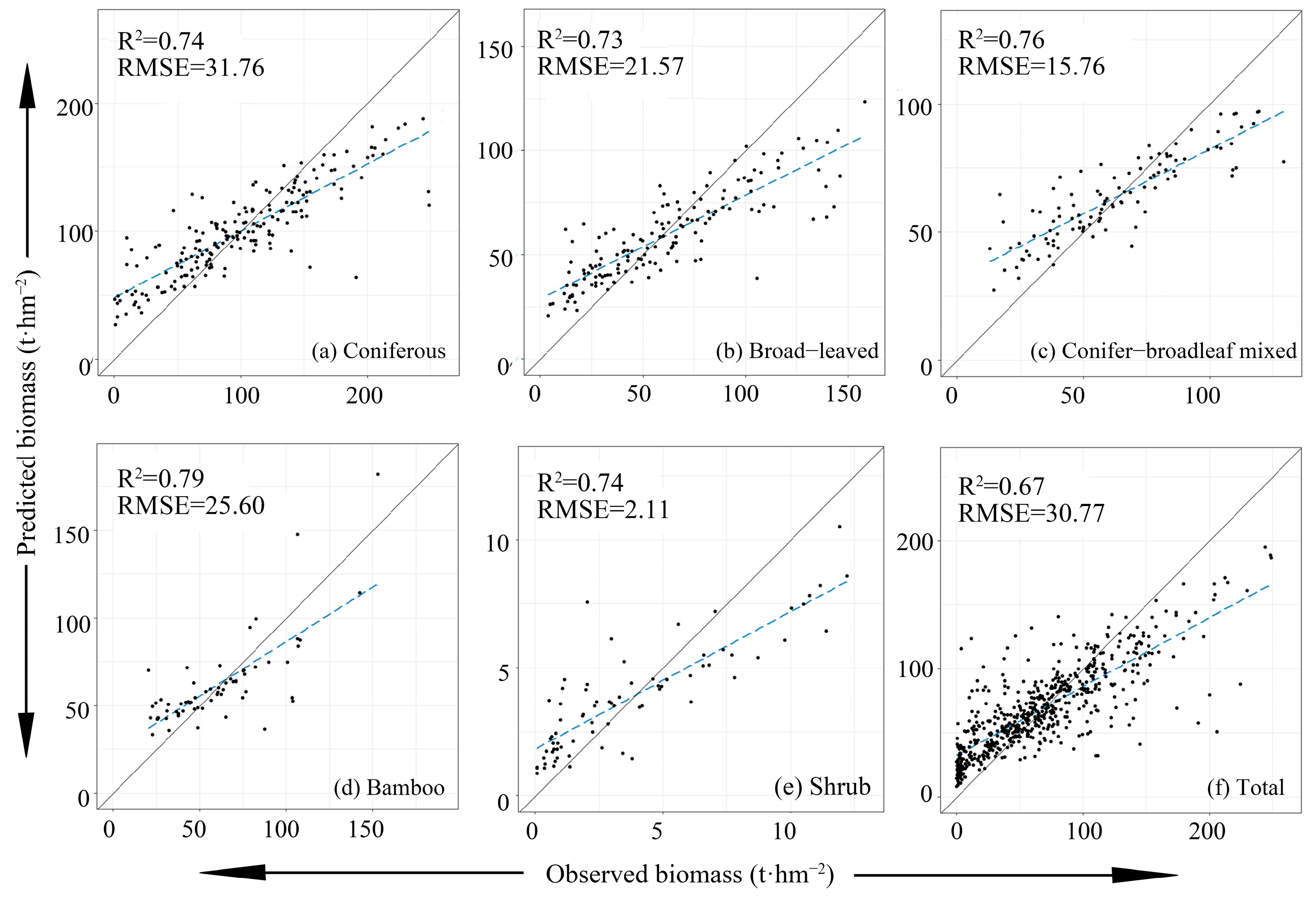
Figure 3.
Predicted biomass distribution using RF models.
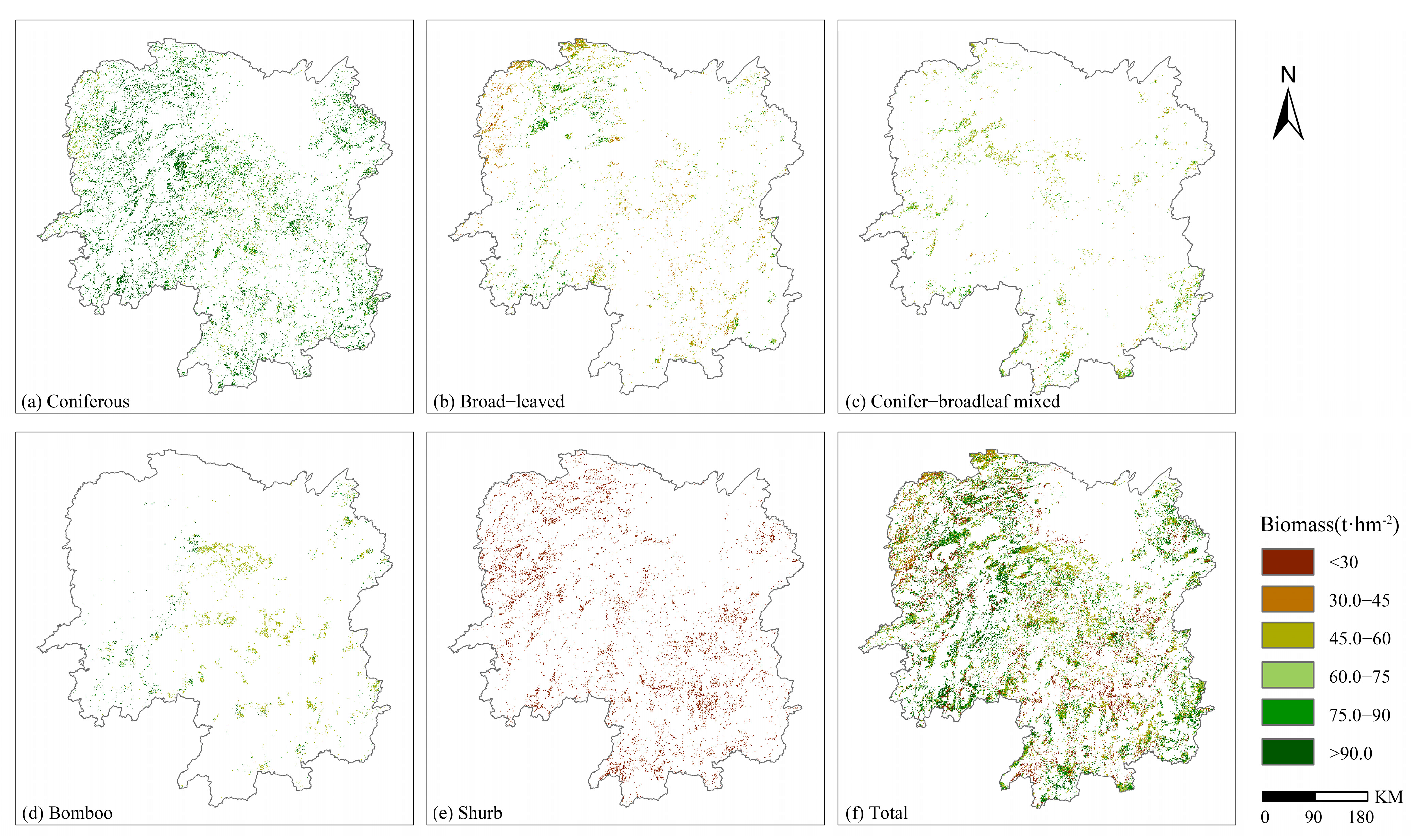
Figure 4.
The area and proportion of each type of biomass.
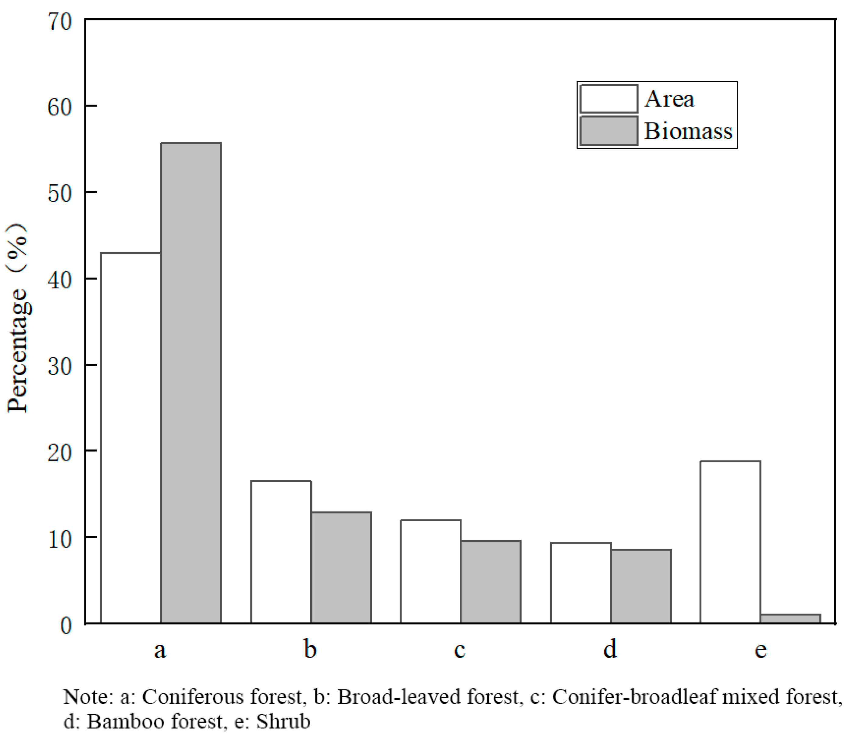
Figure 5.
Spatial distribution coefficient of GWR model in total forest. Note: (a) Spatial distribution of Elevation coefficients; (b) Spatial distribution of Slope coefficients; (c) Spatial distribution of Aspect coefficients; (d) Spatial distribution of GDP coefficients; (e) Spatial distribution of POP coefficients; (f) Spatial distribution of Intercept coefficients.

Table 1.
Basic description of the study area.
| Vegetation Type | Area of Public Welfare Forest (Million hm2) | Percentage (%) | Main Plant Communities |
|---|---|---|---|
| Coniferous forest | 2.14 | 43.16 | Larix gmelinii, Pinus armandii Franch., Pinus massoniana Lamb., Cunninghamia lanceolata, Cupressus funebris, Cryptomeria fortunei, etc. |
| Broadleaf forest | 0.82 | 16.51 | Cinnamomum camphora, Quercus spp., Liquidambar formosana, Sassafras tzumu (Hemsl.) Hemsl., Schima superba Gardn. et Champ, etc. |
| Conifer–broadleaf mixed forest | 0.59 | 11.96 | Pinus massoniana Lamb., Cunninghamia lanceolata, Cupressus funebris, etc. |
| Bamboo forest | 0.47 | 9.43 | Phyllostachys edulis, etc. |
| Shrub | 0.93 | 18.93 | - |
| Total forest | 4.95 | 100 | - |
Table 2.
Statistical results of biomass in the sampling plots.
| Vegetation Type | Sampling Plot Amount | Maximum Biomass (t·hm−2) | Minimum Biomass (t·hm−2) | Mean Biomass (t·hm−2) |
|---|---|---|---|---|
| Coniferous forest | 199 | 324.37 | 0.40 | 107.67 |
| Broadleaf forest | 193 | 198.21 | 3.81 | 72.44 |
| Conifer–broadleaf mixed forest | 139 | 345.66 | 2.92 | 79.62 |
| Bamboo forest | 64 | 415.02 | 20.45 | 65.99 |
| Shrub | 87 | 35.47 | 0.01 | 5.56 |
| Total forest | 682 | 415.02 | 0.01 | 75.04 |
Table 3.
Summary of the spectral variables (SV).
| SV | Definitions of SV | # of SV |
|---|---|---|
| Original band | Coastal aerosol (Band1), blue (Band2), green (Band3), red (Band4), near infrared (Band5), shortwave infrared 1 (Band6), and shortwave infrared 2 (Band7) | 7 |
| Band combinations | Albedo, B4/Albedo, B24 = Band2/Band4, B53 = Band5/Band3, B74 = Band7/Band4, B547 = Band5(Band4/Band7), B345 = Band3(Band4/Band5), and sum visible bands (VIS234) | 8 |
| Image transformations | Principal component analysis (PCA), maximum noise fraction (MNF), high-pass filter (HIP), and low-pass filter (LOP) of seven original bands | 28 |
| Vegetation indices | Normalized difference vegetation index (NDVI), difference vegetation index (DVI), soil adjusted vegetation index (SAVI), simple ratio index (RVI), perpendicular vegetation index (PVI), modified soil adjusted vegetation index (MSAVI), transformation vegetation index (TVI), transformation vegetation index 2 (TVI2), atmospherically resistant vegetation index (ARVI), ND43 = (Band4 − Band3)/(Band4 + Band3), specific leaf area vegetation index (SLAVI), enhanced vegetation index (EVI), green normalized difference vegetation index (GNDVI), modified NLI (MNLI), optimized soil adjusted vegetation index (OSAVI), and renormalized difference vegetation index (RDVI) | 16 |
| Texture measures | Grey-level co-occurrence matrix-based texture measures, including mean, angular second moment, contrast, correlation, dissimilarity, entropy, homogeneity, and variance using moving window sizes of 3 × 3 | 56 |
Table 4.
Selection of driving factors of forest biomass.
| Indicator | Indicators Name | Unit | Resolution | Year |
|---|---|---|---|---|
| Topography | Elevation | m | 30 m × 30 m | 2021 |
| Slope | degrees | 30 m × 30 m | 2021 | |
| Aspect | - | 30 m × 30 m | 2021 | |
| Socio-economic | Gross domestic product (GDP) | 103 CNY/km2 | 1 km × 1 km | 2020 |
| Populations (POP) | people/ km2 | 1 km × 1 km | 2020 | |
| Climate | Temperature | °C | 1 km × 1 km | 2021 |
| Precipitation | mm | 1 km × 1 km | 2021 |
Table 5.
Variables selected based on Boruta algorithm.
| Vegetation Type | Variables Selected |
|---|---|
| Coniferous forest | ARVI, B4,B4/Albedo, B53, B345, GNDVI, MNFB5, NDVI, OSAVI, RVI, SAVI, SLAVI, TVI, PCAB2, PCAB5, HomB5, ConB5, DisB5, VarB6, ConB6, and DisB6 |
| Broadleaf forest | ARVI, B4/Albedo, B53, GNDVI, MNFB2, MNFB7, NDVI, OSAVI, RVI, SAVI, SLAVI, TVI, TVI2, PCAB2, and PCAB6 |
| Conifer–broadleaf mixed forest | B7, B53, MNFB3, MNFB5, SLAVI, PCAB3, PCAB5, and MeaB7 |
| Bamboo forest | ARVI, ND43, SLAVI, PCAB2, HomB7, ConB7, DisB7, EntB7, ASMB7 |
| Shrub | ARVI, B24, MeaB7, RDVI1, and SLAVI |
| Total forest | Albedo, ARVI, B2, B3, B4, B4/Albedo, B6, B7, B53, B74, B345, B547, DVI, EVI, GNDVI, MNFB2, MNFB3, MNFB5, MSAVI, ND43, NDVI, OSAVI, PVI, RDVI1, RVI, SAVI, SLAVI, TVI, TVI2, VIS234, PCAB1, PCAB2, PCAB4, PCAB5, MeaB5, MeaB6, and MeaB7 |
Table 6.
Biomass statistics of each vegetation type under random forest model.
| Vegetation Type | Mean Biomass (t·hm−2) | Biomass (Million Tons) | Percentage (%) |
|---|---|---|---|
| Coniferous forest | 100.33 | 215.24 | 63.62 |
| Broadleaf forest | 59.27 | 48.45 | 14.32 |
| Conifer–broadleaf mixed forest | 62.44 | 36.97 | 10.93 |
| Bamboo forest | 71.33 | 33.32 | 9.85 |
| Shrub | 4.65 | 4.33 | 1.28 |
| Total forest | 68.31 | 338.31 | 100.00 |
Table 7.
Tests of collinearity and significance.
| Vegetation Type | Driving Factors | VIF | p Value |
|---|---|---|---|
| Coniferous forest | Elevation | 1.260 | 0.000 |
| Slope | 1.150 | 0.000 | |
| POP | 1.111 | 0.000 | |
| Aspect | 1.000 | 0.000 | |
| GDP | 1.065 | 0.001 | |
| Broadleaf forest | Elevation | 1.024 | 0.000 |
| POP | 1.039 | 0.038 | |
| GDP | 1.057 | 0.041 | |
| Conifer–broadleaf mixed forest | Elevation | 1.152 | 0.000 |
| Aspect | 1.000 | 0.000 | |
| GDP | 1.066 | 0.007 | |
| POP | 1.094 | 0.104 | |
| Slope | 1.094 | 0.736 | |
| Bamboo forest | Elevation | 1.154 | 0.000 |
| GDP | 1.061 | 0.000 | |
| POP | 1.056 | 0.015 | |
| Shrub | Slope | 1.231 | 0.000 |
| GDP | 1.030 | 0.000 | |
| POP | 1.061 | 0.001 | |
| Aspect | 1.001 | 0.020 |
Table 8.
Evaluation of geographically weighted regression model and regression coefficient statistics of impact factors.
Table 8.
Evaluation of geographically weighted regression model and regression coefficient statistics of impact factors.
| Regression Coefficient of Coniferous Forest | Regression Coefficient of Conifer–Broadleaf Mixed Forest | ||||||||||||
| Min | Lower-Quartile | Median | Mean | Upper-Quartile | Max | Min | Lower-Quartile | Median | Mean | Upper-Quartile | Max | ||
| Intercept | 56.117 | 75.917 | 95.178 | 89.009 | 115.518 | 135.319 | Intercept | 37.619 | 46.982 | 56.345 | 62.188 | 65.708 | 75.070 |
| Elevation | −0.849 | −0.049 | −0.015 | 0.010 | 0.020 | 0.055 | Elevation | −0.029 | −0.018 | −0.007 | −0.001 | 0.003 | 0.014 |
| Slope | −0.537 | −0.156 | 0.225 | 0.303 | 0.606 | 0.988 | Slope | −0.236 | −0.032 | 0.171 | 0.016 | 0.375 | 0.579 |
| Aspect | −0.025 | 0.009 | 0.042 | 0.022 | 0.076 | 0.109 | Aspect | −0.016 | −0.005 | 0.006 | 0.008 | 0.018 | 0.029 |
| POP | −0.030 | −0.014 | 0.002 | −0.003 | 0.019 | 0.036 | POP | −0.038 | −0.025 | −0.013 | −0.003 | 0.004 | 0.013 |
| GDP | −0.074 | −0.045 | −0.016 | −0.004 | 0.013 | 0.043 | GDP | −0.023 | −0.015 | −0.008 | −0.004 | −0.000 | 0.007 |
| R2 = 0.29 | AICc = 161,796.21 | R2 = 0.39 | AICc = 56,279.68 | ||||||||||
| Regression Coefficient of Broadleaf Forest | Regression Coefficient of Bamboo Forest | ||||||||||||
| Min | Lower-Quartile | Median | Mean | Upper-Quartile | Max | Min | Lower-Quartile | Median | Mean | Upper-Quartile | Max | ||
| Intercept | 14.06 | 31.329 | 48.602 | 56.179 | 65.875 | 83.148 | Intercept | 32.180 | 52.224 | 72.267 | 66.305 | 92.310 | 112.364 |
| Elevation | −0.048 | −0.028 | −0.008 | 0.003 | 0.011 | 0.031 | Elevation | −0.106 | −0.063 | −0.019 | 0.009 | 0.025 | 0.069 |
| POP | −0.060 | −0.042 | −0.024 | −0.008 | −0.006 | 0.0122 | POP | −2.170 | −1.584 | −0.999 | −0.010 | −0.413 | 0.173 |
| GDP | −0.116 | −0.005 | 0.000 | 0.000 | 0.007 | 0.013 | GDP | −0.035 | 0.006 | 0.048 | −0.001 | 0.089 | 0.131 |
| R2 = 0.27 | AICc = 58,586.15 | R2 = 0.41 | AICc = 32,622.50 | ||||||||||
| Regression Coefficient of Shrub Forest | Regression Coefficient of Total Forest | ||||||||||||
| Min | Lower-Quartile | Median | Mean | Upper-Quartile | Max | Min | Lower-Quartile | Median | Mean | Upper-Quartile | Max | ||
| Intercept | −5.282 | 1.885 | 4.299 | 4.205 | 6.712 | 9.126 | Intercept | −7.7434 | 41.8186 | 71.9099 | 70.8741 | 99.0510 | 142.7129 |
| Slope | −0.078 | −0.027 | 0.024 | 0.022 | 0.075 | 0.126 | Elevation | −0.0772 | −0.0238 | −0.0006 | 0.0001 | 0.0224 | 0.1068 |
| Aspect | −0.005 | −0.002 | 0.000 | 0.001 | 0.002 | 0.005 | Slope | −0.9861 | −00.240 | 0.1143 | 0.0808 | 0.5353 | 1.4539 |
| POP | −0.005 | −0.003 | −0.001 | −0.001 | 0.002 | 0.004 | Aspect | −0.0463 | −0.0072 | 0.0085 | 0.0078 | 0.0233 | 0.0588 |
| GDP | −0.010 | −0.006 | −0.003 | −0.001 | 0.000 | 0.004 | POP | −0.0785 | −0.0224 | −0.0077 | −0.0053 | 0.0044 | 0.0316 |
| R2 = 0.48 | AICc = 29,331.82 | GDP | −0.1260 | −0.0174 | 0.0145 | −0.0010 | 0.0635 | 0.1281 | |||||
Table 9.
Geographically weighted regression factor regression coefficient proportion segment statistics.
Table 9.
Geographically weighted regression factor regression coefficient proportion segment statistics.
| Elevation | GDP | |||||||||
| <−0.033 | [−0.033, 0) | [0, 0.008) | [0.008, 0.025) | >0.025 | <−0.033 | [−0.033, −0.016) | [−0.016, 0) | [0, 0.011) | >0.011 | |
| Coniferous forest | 2.33 | 21.91 | 18.61 | 39.71 | 17.43 | 2.98 | 8.27 | 48.38 | 37.41 | 2.96 |
| Broadleaf forest | 0.78 | 47.88 | 8.54 | 32.84 | 9.97 | - | - | 45.37 | 54.09 | 0.54 |
| Conifer–broadleaf mixed forest | - | 49.44 | 43.27 | 7.29 | - | - | 9.16 | 66.73 | 24.11 | - |
| Bamboo forest | 0.50 | 27.50 | 34.70 | 17.90 | 19.40 | - | 5.70 | 58.60 | 26.70 | 9.00 |
| Shrub | - | - | - | - | - | - | 0 | 66.03 | 35.97 | 0 |
| Total forest | 1.26 | 36.23 | 24.44 | 25.69 | 12.38 | 1.55 | 5.54 | 53.51 | 37.07 | 2.33 |
| Aspect | Slope | |||||||||
| <−0.023 | [−0.023, 0) | [0, 0.011) | [0.011, 0.029) | >0.029 | <−0.070 | [−0.070, 0) | [0, 0.326) | [0.326, 0.592) | >0.592 | |
| Coniferous forest | 0.10 | 4.61 | 13.30 | 49.90 | 32.09 | 6.83 | 5.42 | 39.84 | 32.72 | 15.18 |
| Conifer–broadleaf mixed forest | - | 23.74 | 33.83 | 42.24 | 0.19 | 17.45 | 37.68 | 43.91 | 0.96 | - |
| Shrub | - | 36.25 | 63.75 | - | - | - | 14.31 | 85.69 | 0 | - |
| Total forest | 5.54 | 0.57 | 30.21 | 29.35 | 34.32 | 9.31 | 13.90 | 50.20 | 19.12 | 7.48 |
| POP | Intercept | |||||||||
| <−0.015 | [−0.015, −0.006) | [−0.006, 0) | [0, 0.020) | >0.020 | [0, 32.25) | [32.25, 72.55) | [72.55, 94.71) | [94.71, 130.98) | >130.974 | |
| Coniferous forest | 5.99 | 22.28 | 41.96 | 29.27 | 0.50 | - | 15.34 | 48.89 | 35.56 | 0.21 |
| Broadleaf forest | 15.04 | 23.48 | 42.32 | 19.16 | - | - | 79.85 | 20.15 | - | - |
| Conifer–broadleaf mixed forest | - | 3.65 | 28.25 | 35.08 | 33.02 | - | 89.25 | 10.75 | - | 0 |
| Bamboo forest | 11.99 | 20.50 | 40.48 | 21.66 | 5.36 | 72.02 | 25.00 | 2.98 | - | - |
| Shrub | - | - | 92.09 | 7.91 | - | 100 | - | - | - | - |
| Total forest | 7.48 | 20.08 | 48.58 | 23.24 | 0.63 | 19.75 | 34.88 | 24.15 | 16.26 | 4.97 |
Disclaimer/Publisher’s Note: The statements, opinions and data contained in all publications are solely those of the individual author(s) and contributor(s) and not of MDPI and/or the editor(s). MDPI and/or the editor(s) disclaim responsibility for any injury to people or property resulting from any ideas, methods, instructions or products referred to in the content. |
© 2023 by the authors. Licensee MDPI, Basel, Switzerland. This article is an open access article distributed under the terms and conditions of the Creative Commons Attribution (CC BY) license (https://creativecommons.org/licenses/by/4.0/).
Share and Cite
MDPI and ACS Style
Liu, H.; Fu, Y.; Pan, J.; Wang, G.; Hu, K. Biomass Spatial Pattern and Driving Factors of Different Vegetation Types of Public Welfare Forests in Hunan Province. Forests 2023, 14, 1061. https://doi.org/10.3390/f14051061
AMA Style
Liu H, Fu Y, Pan J, Wang G, Hu K. Biomass Spatial Pattern and Driving Factors of Different Vegetation Types of Public Welfare Forests in Hunan Province. Forests. 2023; 14(5):1061. https://doi.org/10.3390/f14051061
Chicago/Turabian StyleLiu, Huiting, Yue Fu, Jun Pan, Guangjun Wang, and Kongfei Hu. 2023. "Biomass Spatial Pattern and Driving Factors of Different Vegetation Types of Public Welfare Forests in Hunan Province" Forests 14, no. 5: 1061. https://doi.org/10.3390/f14051061
Note that from the first issue of 2016, this journal uses article numbers instead of page numbers. See further details here.