
Spatial Patterns and Associations of Tree Species in a Temperate Forest of National Forest Park, Huadian City, Jilin Province, Northeast China

Abstract
:1. Introduction
2. Methods
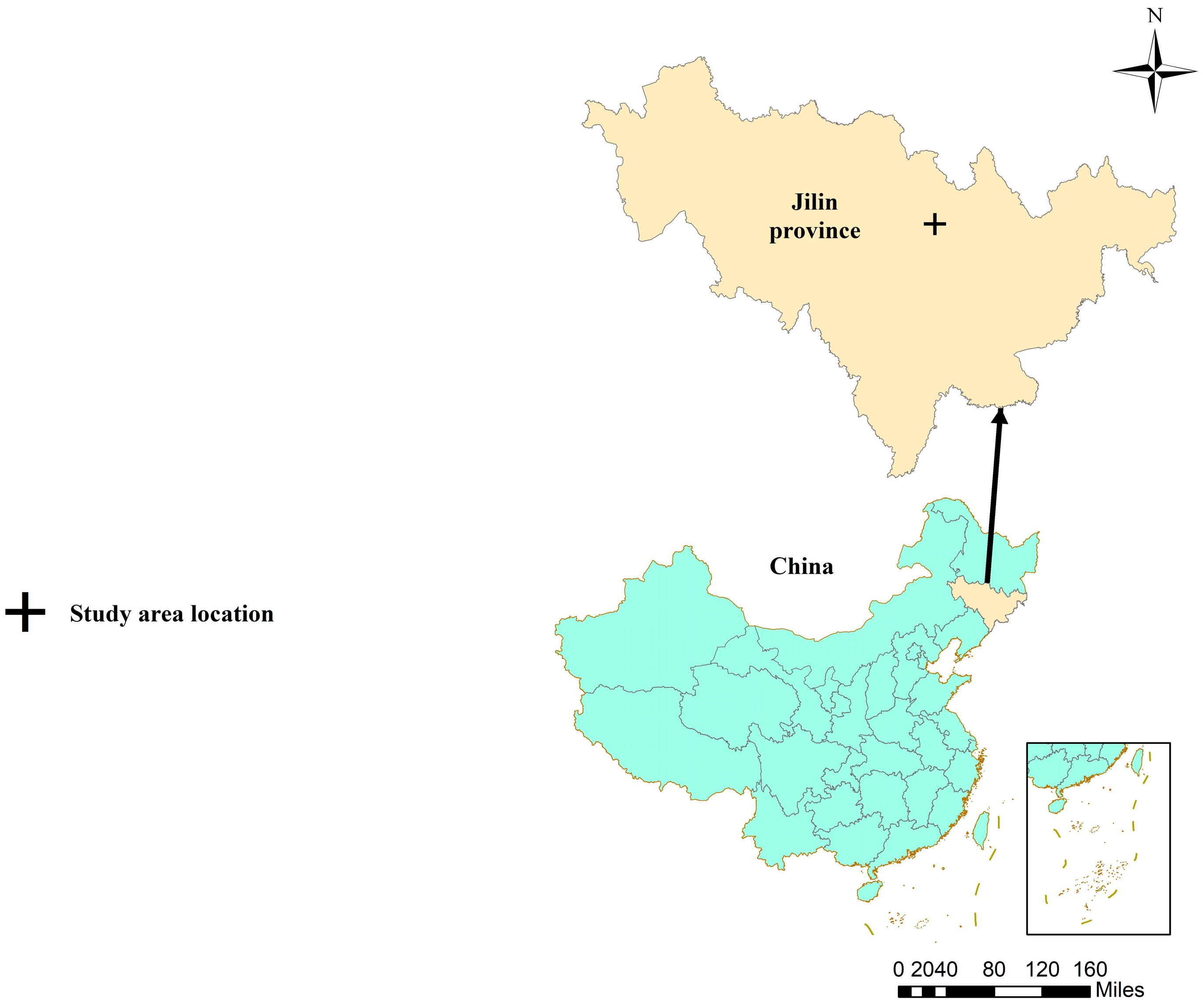
2.1. Study Site
2.2. Data Collection
2.3. Data Analysis
3. Results
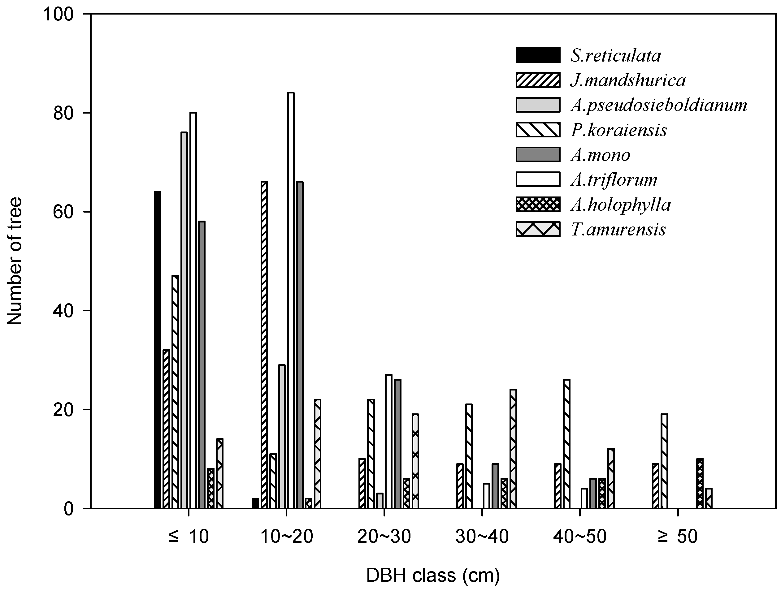
3.1. Population Structure
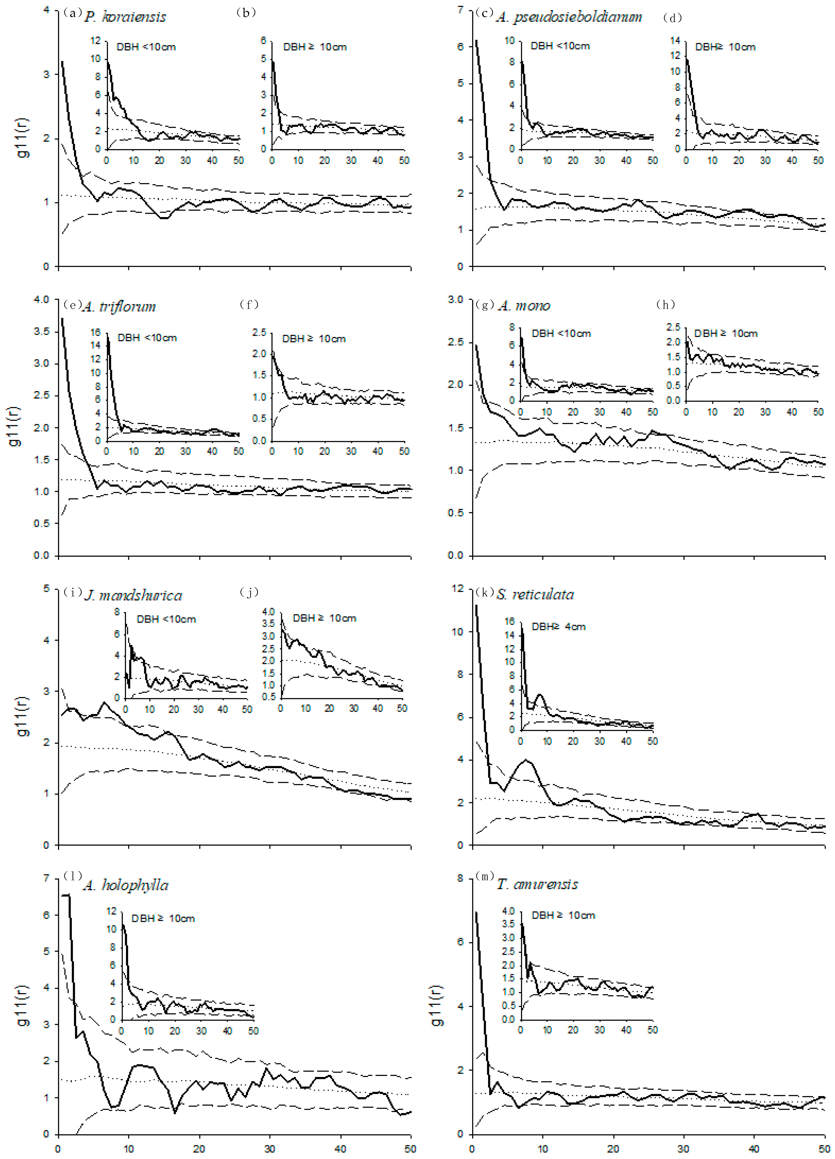
3.2. Spatial Patterns
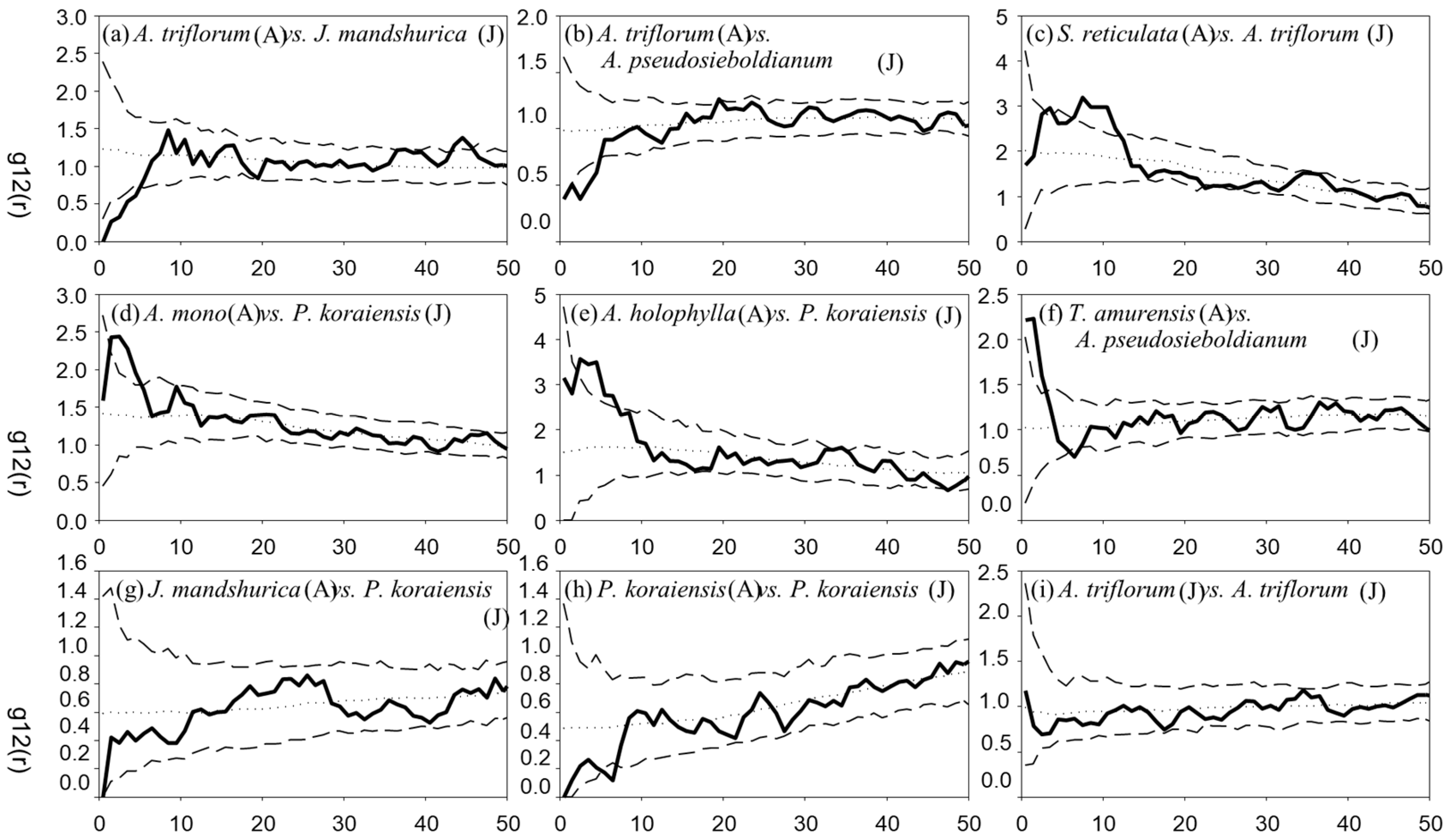
3.3. Spatial Associations
4. Discussion
4.1. Spatial Distribution Patterns and Influencing Factors
4.2. Methodological Limitations
4.3. Implications for Conservation
5. Conclusions
Author Contributions
Funding
Data Availability Statement
Acknowledgments
Conflicts of Interest
References
- Raj, A.; Jhariya, M.K.; Banerjee, A.; Lal, B.; Mechergui, T.; Devi, A. Ghanshyam Forest for Sustainable Development. In Land and Environmental Management through Forestry; Wiley: Hoboken, NJ, USA, 2023; pp. 293–311. [Google Scholar]
- Dreiss, L.M.; Volin, J.C. Forests: Temperate evergreen and deciduous. In Terrestrial Ecosystems and Biodiversity; CRC Press: Boca Raton, FL, USA, 2020; pp. 213–226. [Google Scholar]
- Palaghianu, C.; Coșofreț, C. Patterns of Forest Species Association in a Broadleaf Forest in Romania. Forests 2023, 14, 1118. [Google Scholar] [CrossRef]
- Zhang, M.; Wang, J.; Kang, X. Spatial distribution pattern of dominant tree species in different disturbance plots in the Changbai Mountain. Sci. Rep. 2022, 12, 14161. [Google Scholar] [CrossRef]
- Perea, A.J.; Wiegand, T.; Garrido, J.L.; Rey, P.J.; Alcántara, J.M. Spatial phylogenetic and phenotypic patterns reveal ontogenetic shifts in ecological processes of plant community assembly. Oikos 2022, 2022, e09260. [Google Scholar] [CrossRef]
- Watt, A.S. Pattern and process in the plant community. J. Ecol. 1947, 35, 1–22. [Google Scholar] [CrossRef]
- Gratzer, G.; Waagepetersen, R.P. Seed Dispersal, Microsites or Competition—What Drives Gap Regeneration in an Old-Growth Forest? An Application of Spatial Point Process Modelling. Forests 2018, 9, 230. [Google Scholar] [CrossRef]
- Pang, S.E.; Ferry Slik, J.W.; Zurell, D.; Webb, E.L. The clustering of spatially associated species unravels patterns in Bornean tree species distributions. bioRxiv 2022. [Google Scholar] [CrossRef]
- Xu, C.; Zhao, S.; Liu, S. Spatial scaling of multiple landscape features in the conterminous United States. Landsc. Ecol. 2020, 35, 223–247. [Google Scholar] [CrossRef]
- Jin, L.S.; Yin, D.; Fortin, M.J.; Cadotte, M.W. The mechanisms generating community phylogenetic patterns change with spatial scale. Oecologia 2020, 193, 655–664. [Google Scholar] [CrossRef] [PubMed]
- Zhou, Q.; Shi, H.; Shu, X.; Xie, F.; Zhang, K.; Zhang, Q.; Dang, H. Spatial distribution and interspecific associations in a deciduous broad-leaved forest in north-central China. J. Veg. Sci. 2019, 30, 1153–1163. [Google Scholar] [CrossRef]
- Holmes, M.A.; Matlack, G.R. Spatial structure develops early in forest herb populations, controlled by dispersal and life cycle. Oecologia 2019, 189, 951–970. [Google Scholar] [CrossRef]
- Ta, F.; Liu, X.D.; Liu, R.H.; Zhao, W.J.; Jing, W.M.; Ma, J.; Wu, X.R.; Zhao, J.-Z.; Ma, X. Spatial distribution patterns and association of Picea crassifolia population in Dayekou Basin of Qilian Mountains, northwestern China. Chin. J. Plant Ecol. 2020, 44, 1172. [Google Scholar] [CrossRef]
- Deng, C.; Guan, Y.; Waagepetersen, R.P.; Zhang, J. Second-order quasi-likelihood for spatial point processes. Biometrics 2017, 73, 1311–1320. [Google Scholar] [CrossRef] [PubMed]
- Ben-Said, M. Spatial point-pattern analysis as a powerful tool in identifying pattern-process relationships in plant ecology: An updated review. Ecol. Process. 2021, 10, 56. [Google Scholar] [CrossRef]
- Ma, Z.B.; Xiao, W.F.; Huang, Q.L.; Zhuang, C.Y. A review of point pattern analysis in ecology and its application in China. Acta Ecol. Sin. 2017, 37, 6624–6632. [Google Scholar]
- Condit, R. Research in large, long-term tropical forest plots. Trends Ecol. Evol. 1995, 10, 18–22. [Google Scholar] [CrossRef]
- Harms, K.E.; Wright, S.J.; Calderón, O.; Hernandez, A.; Herre, E.A. Pervasive density-dependent recruitment enhances seedling diversity in a tropical forest. Nature 2000, 404, 493–495. [Google Scholar] [CrossRef]
- Hubbell, S. The Unified Neutral Theory of Biodiversity and Biogeography; Princeton University Press: Princeton, NJ, USA, 2001; p. 32. [Google Scholar]
- McMillan, N.A.; Fuhlendorf, S.D.; Davis, C.A.; Hamilton, R.G.; Neumann, L.K.; Cady, S.M. A plea for scale, and why it matters for invasive species management, biodiversity and conservation. J. Appl. Ecol. 2023, 60, 1468–1480. [Google Scholar] [CrossRef]
- Keyimu, M.; Halik, U.; Betz, F.; Wumaier, G.; Dilimulati, G. Spatial-temporal change of DBH of Populus euphratica under artificial water conveyances. J. For. Environ. 2016, 36, 148. [Google Scholar]
- Yang, H.B.; Guo, Q.X. Influence of topography and competitive factors on the relationship between DBH and age of Korean pine. Acta Ecol. Sin. 2016, 36, 6487–6495. [Google Scholar]
- Liu, J.; Bai, X.; Yin, Y.; Wang, W.; Li, Z.; Ma, P. Spatial patterns and associations of tree species at different developmental stages in a montane secondary temperate forest of northeastern China. PeerJ 2021, 9, e11517. [Google Scholar] [CrossRef]
- Peralta, A.L.; Escudero, A.; de la Cruz, M.; Sánchez, A.M.; Luzuriaga, A.L. Functional traits explain both seedling and adult plant spatial patterns in gypsum annual species. Funct. Ecol. 2023, 37, 1170–1180. [Google Scholar] [CrossRef]
- Ulrich, W.; Zaplata, M.K.; Winter, S.; Fischer, A. Spatial distribution of functional traits indicates small scale habitat filtering during early plant succession. Perspect. Plant Ecol. Evol. Syst. 2017, 28, 58–66. [Google Scholar] [CrossRef]
- Watanabe, S.; Maesako, Y. Co-occurrence pattern of congeneric tree species provides conflicting evidence for competition relatedness hypothesis. PeerJ 2021, 9, e12150. [Google Scholar] [CrossRef] [PubMed]
- D’Andrea, R.; O’Dwyer, J.P. Competition for space in a structured landscape: The effect of seed limitation on coexistence under a tolerance-fecundity trade-off. J. Ecol. 2021, 109, 1886–1897. [Google Scholar] [CrossRef]
- Traoré, A.S.; Kouassi, K.I.; Koné, M.; Gignoux, J.; Barot, S. Spatial patterns of a savanna palm tree Borassus aethiopum and its temporal variability. J. Plant Ecol. 2022, 15, 1049–1064. [Google Scholar] [CrossRef]
- Wang, C.; Jiang, Q.O.; Deng, X.; Lv, K.; Zhang, Z. Spatio-temporal evolution, future trend and phenology regularity of net primary productivity of forests in Northeast China. Remote Sens. 2020, 12, 3670. [Google Scholar] [CrossRef]
- Gu, Y.; Zhang, J.; Ma, W.; Feng, Y.; Yang, L.; Li, Z.; Guo, Y.; Shi, G.; Han, S. Ecological Factors Driving Tree Diversity across Spatial Scales in Temperate Forests, Northeast China. Forests 2023, 14, 1241. [Google Scholar] [CrossRef]
- Liao, Z.; Su, K.; Jiang, X.; Zhou, X.; Yu, Z.; Chen, Z.; Wei, C.; Zhang, Y.; Wang, L. Ecosystem and Driving Force Evaluation of Northeast Forest Belt. Land 2022, 11, 1306. [Google Scholar] [CrossRef]
- Zhang, J.; Hao, Z.Q.; Song, B.; Ye, J.; Li, B.H.; Yao, X.L. Spatial distribution patterns and associations of Pinus koraiensis and Tilia amurensis in broad-leaved Korean pine mixed forest in Changbai Mountains. Chin. J. Appl. Ecol. 2007, 18, 1681–1687. [Google Scholar]
- Omelko, A.; Ukhvatkina, O.; Zhmerenetsky, A.; Sibirina, L.; Petrenko, T.; Bobrovsky, M. From young to adult trees: How spatial patterns of plants with different life strategies change during age development in an old-growth Korean pine-broadleaved forest. For. Ecol. Manag. 2018, 411, 46–66. [Google Scholar] [CrossRef]
- Zhang, X.P.; Yu, L.Z.; Yang, X.Y.; Huang, J.Q.; Yin, Y. Population structure and dynamics of Pinus koraiensis seedlings regenerated from seeds in a montane region of eastern Liaoning Province, China. Ying Yong Sheng Tai Xue Bao = J. Appl. Ecol. 2022, 33, 289–296. [Google Scholar]
- You, Z.; Wencai, W. Flora of Changbai Mountain, China; China Forestry Publishing House: Beijing, China, 2010. [Google Scholar]
- Bradford, M.; Murphy, H.T. The importance of large-diameter trees in the wet tropical rainforests of Australia. PLoS ONE 2019, 14, e0208377. [Google Scholar] [CrossRef] [PubMed]
- Xu, X.; Su, Z.; Yan, X. Effects of aspect on distribution pattern of Taxus chinensis population in Yele, Sichuan Province: An analysis based on patches information. Ying Yong Sheng Tai Xue Bao= J. Appl. Ecol. 2005, 16, 985–990. [Google Scholar]
- Ripley, B.D. Spatial Statistics; Wiley & Sons: New York, NY, USA, 1981. [Google Scholar]
- Gómez-Rubio, V. Spatial point patterns: Methodology and applications with R. J. Stat. Softw. 2016, 75, 1–6. [Google Scholar] [CrossRef]
- Baddeley, A.; Rubak, E.; Turner, R. Spatial Point Patterns: Methodology and Applications with R; CRC Press: Boca Raton, FL, USA, 2015. [Google Scholar]
- Xiang, Q.; Guo, Q.-j.; Ai, X.-r.; Yao, L.; Zhu, J.; Xue, W.-x.; Zhou, Y.; Zhao, H.-d.; Wu, J.-y. Variations on Stand Spatial Structure and Species Diversity in Different Spatial Scales. For. Res. 2022, 35, 151–160. [Google Scholar]
- Liu, Q.; Wu, Z.W.; Lin, S.T.; Li, S.; Fang, Z.B. Spatial point pattern analysis of pine wilt disease occurrence and its influence factors. Ying Yong Sheng Tai Xue Bao = J. Appl. Ecol. 2022, 33, 2530–2538. [Google Scholar]
- Self, S.; Overby, A.; Zgodic, A.; White, D.; McLain, A.; Dyckman, C. A Generalization of Ripley’s K Function for the Detection of Spatial Clustering in Areal Data. arXiv 2022, arXiv:2204.10852. [Google Scholar]
- Hohl, A.; Zheng, M.; Tang, W.; Delmelle, E.; Casas, I. Spatiotemporal point pattern analysis using Ripley’s K function. In Geospatial Data Science Techniques and Applications; CRC Press: Boca Raton, FL, USA, 2017; pp. 155–176. [Google Scholar]
- Yates, L.A.; Brook, B.W.; Buettel, J.C. Spatial pattern analysis of line-segment data in ecology. Ecology 2022, 103, e03597. [Google Scholar] [CrossRef]
- Condit, R.; Ashton, P.S.; Baker, P.; Bunyavejchewin, S.; Gunatilleke, S.; Gunatilleke, N.; Hubbell, S.P.; Foster, R.B.; Itoh, A.; LaFrankie, J.V.; et al. Spatial Patterns in the Distribution of Tropical Tree Species. Science 2000, 288, 1414–1418. [Google Scholar] [CrossRef]
- Wiegand, T.A.; Moloney, K. Rings, circles, and null-models for point pattern analysis in ecology. Oikos 2004, 104, 209–229. [Google Scholar] [CrossRef]
- Villegas, P.; Cavagna, A.; Cencini, M.; Fort, H.; Grigera, T.S. Joint assessment of density correlations and fluctuations for analysing spatial tree patterns. R. Soc. Open Sci. 2021, 8, 202200. [Google Scholar] [CrossRef]
- Qu, H.; Zhang, Q. A method to improve Ripley’s function to analyze spatial pattern by factor analysis. In Proceedings of theInternational Conference on Electronic Information Engineering and Data Processing (EIEDP 2023), SPIE, Nanchang, China, 17–19 March 2023; Volume 12700, pp. 562–566. [Google Scholar]
- Wang, X.T.; Wang, D.J.; Li, H.B.; Tai, Y.; Jiang, C.; Liu, F.; Li, S.Y.; Miao, B.L. Cumulative effects of K-function in the research of point patterns. Ying Yong Sheng Tai Xue Bao = J. Appl. Ecol. 2022, 33, 1275–1282. [Google Scholar]
- Wiegand, T.; Gunatilleke, S.; Gunatilleke, N. Species associations in a heterogeneous Sri Lankan dipterocarp forest. Am. Nat. 2007, 170, E77–E95. [Google Scholar] [CrossRef] [PubMed]
- Zimback, L.B. Quais características influenciam a limitação de dispersão de sementes em uma comunidade arbórea tropical? Master’s Thesis, Universidade de São Paulo, São Paulo, Brazil, 2017. [Google Scholar]
- Gharti, P.; Dani, R.S.; Baniya, C.B. Relationship of topography and soil chemistry with plant richness and distribution in the temperate forest of Chandragiri hill, Kathmandu, Nepal. Res. Sq. 2023. [Google Scholar] [CrossRef]
- Lara-Romero, C.; de la Cruz, M.; Escribano-Ávila, G.; García-Fernández, A.; Iriondo, J.M. What causes conspecific plant aggregation? Disentangling the role of dispersal, habitat heterogeneity and plant–plant interactions. Oikos 2016, 125, 1304–1313. [Google Scholar] [CrossRef]
- Anacker, B.L.; Strauss, S.Y. Ecological similarity is related to phylogenetic distance between species in a cross-niche field trans-plant experiment. Ecology 2016, 97, 1807–1818. [Google Scholar] [CrossRef] [PubMed]
- Eigentler, L. Species coexistence in resource-limited patterned ecosystems is facilitated by the interplay of spatial self-organisation and intraspecific competition. Oikos 2021, 130, 609–623. [Google Scholar] [CrossRef]
- Keddy, P.A. Competition. In Causal Factors for Wetland Management and Restoration: A Concise Guide; Keddy, P.A., Ed.; Springer International Publishing: Cham, Switzerland, 2023; pp. 73–80. [Google Scholar]
- Qi, Y.; Zhang, G.; Xiong, Z.; Yang, T. Spatial point pattern analysis for coarse woody debris in karst mixed evergreen and deciduous broadleaved forest. Acta Ecol. Sin. 2019, 39, 4933–4943. [Google Scholar]
- Gizachew, G. Spatial-temporal and factors influencing the distribution of biodiversity: A review. ASEAN J. Sci. Eng. 2022, 2, 273–284. [Google Scholar] [CrossRef]


| Species 1 | Species 2 | p Values | Scales (m) | |||||||
|---|---|---|---|---|---|---|---|---|---|---|
| 0–5 | 5–10 | 10–15 | 15–20 | 20–25 | 25–30 | 30–40 | 40–50 | |||
| S. reticulata | J. mandshurica | 0.0005 | +(no) | +(no) | no | no | no(−) | no | no | no |
| J. mandshurica | S. reticulata | 0.01 | + | + | no | no | no | no | no | no(−) |
| J. mandshurica | A. pseudosieboldianum | 0.035 | −(no) | no(−) | no | no | no | no | no | no |
| P. koraiensis | A. pseudosieboldianum | 0.02 | no | +(no) | no | no(−) | no | no | no(+) | no |
| P. koraiensis | A. mono | 0.005 | +(no) | no | no(+) | no | no | no | no | no |
| P. koraiensis | A. holophylla | 0.005 | +(no) | no(+) | no | no | no | no | no | no |
| A. mono | P. koraiensis | 0.015 | +(no) | no | no | no | no | no | no | no |
| A. holophylla | P. koraiensis | 0.005 | +(no) | no(+) | no | no | no | no | no | no |
| A. triflorum | A. pseudosieboldianum | 0.005 | − | no(−) | no | no | no | no | no | no |
| A. pseudosieboldianum | A. triflorum | 0.02 | −(no) | no | no | no | no | no | no | no |
Disclaimer/Publisher’s Note: The statements, opinions and data contained in all publications are solely those of the individual author(s) and contributor(s) and not of MDPI and/or the editor(s). MDPI and/or the editor(s) disclaim responsibility for any injury to people or property resulting from any ideas, methods, instructions or products referred to in the content. |
© 2024 by the authors. Licensee MDPI, Basel, Switzerland. This article is an open access article distributed under the terms and conditions of the Creative Commons Attribution (CC BY) license (https://creativecommons.org/licenses/by/4.0/).
Share and Cite
Lin, L.; Ren, X.; Shimizu, H.; Wang, C.; Zou, C. Spatial Patterns and Associations of Tree Species in a Temperate Forest of National Forest Park, Huadian City, Jilin Province, Northeast China. Forests 2024, 15, 714. https://doi.org/10.3390/f15040714
Lin L, Ren X, Shimizu H, Wang C, Zou C. Spatial Patterns and Associations of Tree Species in a Temperate Forest of National Forest Park, Huadian City, Jilin Province, Northeast China. Forests. 2024; 15(4):714. https://doi.org/10.3390/f15040714
Chicago/Turabian StyleLin, Longhui, Xin Ren, Hideyuki Shimizu, Chenghuan Wang, and Chunjing Zou. 2024. "Spatial Patterns and Associations of Tree Species in a Temperate Forest of National Forest Park, Huadian City, Jilin Province, Northeast China" Forests 15, no. 4: 714. https://doi.org/10.3390/f15040714