Characterizing the Height Structure and Composition of a Boreal Forest Using an Individual Tree Crown Approach Applied to Photogrammetric Point Clouds

Abstract

Photogrammetric point clouds (PPC) obtained by stereomatching of aerial photographs now have a resolution sufficient to discern individual trees. We have produced such PPCs of a boreal forest and delineated individual tree crowns using a segmentation algorithm applied to the canopy height model derived from the PPC and a lidar terrain model. The crowns were characterized in terms of height and species (spruce, fir, and deciduous). Species classification used the 3D shape of the single crowns and their reflectance properties. The same was performed on a lidar dataset. Results show that the quality of PPC data generally approaches that of airborne lidar. For pixel-based canopy height models, viewing geometry in aerial images, forest structure (dense vs. open canopies), and composition (deciduous vs. conifers) influenced the quality of the 3D reconstruction of PPCs relative to lidar. Nevertheless, when individual tree height distributions were analyzed, PPC-based results were very similar to those extracted from lidar. The random forest classification (RF) of individual trees performed better in the lidar case when only 3D metrics were used (83% accuracy for lidar, 79% for PPC). However, when 3D and intensity or multispectral data were used together, the accuracy of PPCs (89%) surpassed that of lidar (86%).

1. Introduction

Airborne lidar has been used extensively to characterize the structure of forest canopies [1,2,3], and to a lesser extent to identify tree species (e.g., [4,5,6,7,8]). In both cases, two alternative methods were tested: the now classical area-based approach (ABA, e.g., [9]) and the individual tree crown (ITC) methods (see [10], and [11] for reviews). For structural attribute quantification, both ABA and ITC can now achieve results of relatively high accuracy. However, for more species-specific attributes estimations in mixed forests, it can be argued that ABA reaches limitations and ITC methods can theoretically produce more detailed information [12,13] because the point cloud characteristics of individual trees can be linked to species-specific features, such as crown shape, porosity or reflectance [7,14]. ABA on the other hand can only describe overall point cloud features on a plot or stand basis, leading to substantial ambiguity when multiple species are present. ITC also offers the advantage of enabling object-based reconstruction of tree size distributions in forests having a complex structure, such as old growth natural forests. It also has the capacity to characterize species-specific tree size distribution characterization when species can be well identified. For these reasons, and because of the great importance of species data in forest inventories, ecological studies, or carbon stock assessment, we here focus our attention on ITC implementations of species identification based on 3D representations of forest canopies.

ITC has hitherto been applied either to monoscopic high resolution images [15,16,17,18] (see [19] for a review) or to lidar point clouds or canopy height models ([20,21,22,23,24]; see [25] for a review of different algorithms over diverse types of forest). Species identification of individual trees using only the 3D data of lidar has been demonstrated [6] using alpha shapes and height distribution, intensity and textural features derived from canopy height models (CHMs). For example, Holmgren and Persson [4] achieved 95% identification accuracy in separating scots pine and Norway spruce. Brandtberg [5] obtained a 64% accuracy for three deciduous species (oaks, red maple and yellow poplar) in leaf-off conditions, while Ørka et al. [7] reached 88% in the case of dominant trees and 64% for non-dominants when classifying spruce and birch. Moreover, Korpela et al. [8] obtained 88%–90% accuracy when discriminating between pine, spruce and birch. However, reaching high accuracy classification results using only lidar data may not be always possible [26]. This has led researchers to combine lidar data with spectral information extracted from optical multispectral sensor images to improve species classification. Among them, Persson et al. [27] achieved overall accuracies of 90% and Holmgren et al. [28] achieved up to 96% accuracy when classifying scots pine, Norway spruce and deciduous trees. Similar results were obtained by Ørka et al. [29], whereas some studies involving combining lidar and hyperspectral images also achieved good success [30,31].

A largely uninvestigated alternative to using lidar alone or in conjunction with imagery consists of using photogrammetric point clouds (PPC). We here define a PPC as a 3D point cloud extracted by image matching and carrying the multispectral brightness information of the matched images. By subtracting the ground elevations obtained from a high accuracy digital terrain model (DTM) from the elevation component (Z) of a PPC, one obtains a set of XYH colored points where H represents the height of the canopy surface at location XY (planimetric position). These point clouds have been shown to be very similar to those created using lidar, especially when based on high overlap photos acquired from unmanned aerial vehicles [32]. However, photogrammetric results generally appear smoother than corresponding point clouds [33], may not describe the full 3D scene because of occlusions effects, and may contain artefacts caused by mismatch [34].

Due to the recent improvement of image matching algorithms that has brought PPCs to new levels of density and accuracy [35,36], ITC implementations based on PPCs are possibly within reach. While several researchers have reported on the accuracy and practical advantages of PPCs when exploited through the ABA [37,38,39,40,41,42,43], only recently has the possibility of applying ITC approaches to PPCs started to emerge [44,45]; see also [46] for a precursor hybrid approach. Although some non-forest centric studies have documented the accuracy of PPCs with the most advanced image matching algorithms on different surfaces [47,48,49], it is still unclear if the current generation of PPCs provide 3D data sufficient to ensure proper tree delineation, if they are precise enough to reflect the height distribution of single trees, and if they contain reliable 3D and reflectance features for identifying tree species. In these regards, PPC-based ITC results have not been compared to corresponding lidar-based results.

The general objective of the present study was to assess the individual tree information contents of PPCs of a mixed boreal forest by comparing them to a corresponding lidar dataset. More specifically, we analysed the effect of aerial photo viewing geometry and forest structure on the accuracy of the 3D point reconstruction and end results. The latter was comprised of lidar-based and PPC-based ITC delineations, comparisons of tree height and crown area distributions, and assessment of the respective percentages of correct species classification based on both types of data.

2. Materials and Methods

2.1. Study Area

Our analysis was carried out on six sites located in the Montmorency Forest, a study and research facility of Laval University. This forest is located approximately 50 km north of Quebec City, Canada, (47°18′ N, 71°08′ W) in the Canadian boreal shield ecozone [50]. It is composed mainly of balsam firs (Abies balsamea (L.) Miller), but other species such as white spruce (Picea glauca (Moench) Voss), trembling aspen (Populus tremuloides Michaux), and paper birch (Betula papyrifera Marshall) are also common. Due to its relatively high latitude and elevation (approximately 460–1040 meters above sea level), tree height rarely exceeds 20 m. Although a large part of this territory is managed and was harvested at various points in the past, the selected sites essentially contain mature trees with stand ages of 50 to more than 80 years.

Six sites were selected using criteria that were coherent with the experimental design of this study. Our aim was to include sites with different aerial photo view angles, forest structures, and compositions, while limiting the overall number of sites to avoid creating an overwhelming number of viewing geometry, structure, composition, and classification metrics combinations. The selected sites represent dense conifers (DC), open conifers (OC), and dense mixed woods (DM, i.e., combination of conifers and deciduous trees), each with a near vertical (v) and oblique (o) photo viewing geometry (Table 1). This geometry was qualified according to the viewing angle statistics calculated between the position of the camera and the center of each site. Each of these had an area between 3 and 12 ha, and were located on flat or slightly inclined terrain.

Table 1. Description of the six study sites with their approximate coverage and view angles.

Site Name	Description	Area (ha)	Angle (Degrees)
			Mean	Min/Max
DCv	Dense conifers—near vertical view geometry	5	11.94	7.48/16.10
DCo	Dense conifers—oblique view geometry	5	24.98	21.68/31.00
OCv	Open conifers—near vertical view geometry	3	8.37	1.90/15.24
OCo	Open conifers—oblique view geometry	3	18.92	15.46/25.11
DMv	Dense mixed woods—near vertical view geometry	12	8.31	2.42/15.77
DMo	Dense mixed woods—oblique view geometry	12	19.94	17.84/22.65

Table 1. Description of the six study sites with their approximate coverage and view angles.

Site Name	Description	Area (ha)	Angle (Degrees)
			Mean	Min/Max
DCv	Dense conifers—near vertical view geometry	5	11.94	7.48/16.10
DCo	Dense conifers—oblique view geometry	5	24.98	21.68/31.00
OCv	Open conifers—near vertical view geometry	3	8.37	1.90/15.24
OCo	Open conifers—oblique view geometry	3	18.92	15.46/25.11
DMv	Dense mixed woods—near vertical view geometry	12	8.31	2.42/15.77
DMo	Dense mixed woods—oblique view geometry	12	19.94	17.84/22.65

2.2. Remote Sensing Data

The images covering the study sites were acquired on 24 June 2012 with a Microsoft-Vexcel UltraCam XP aerial camera (Vexcel Imaging GmbH, Graz, Austria). Images were delivered as 8 bits pansharpened color-infrared (CIR) and natural color in red, green, and blue (RGB) images with a ground sampling distance (GSD) of approximately 10 cm. The image and flight characteristics are given in Table 2.

Table 2. Camera and flight characteristics of the aerial images.

Camera Characteristics
Model	Microsoft UltraCam XP
Calibrated Focal length	100.5 mm
Pixel size	6 μm panchromatic, 18 μm multispectral
Focal plane size	67.860 mm/103.860 mm
Spectral bands	Blue, Green, Red, Near infrared
Flight characteristics
Altitude	2450 m above ground level
Acquisition date	24 June 2012
Ground sampling distance	Approximately 10 cm panchromatic, 40 cm multispectral
Forward overlap	Approximately 80%
Lateral overlap	Approximately 30%
Average base to height ratio	0.12

Table 2. Camera and flight characteristics of the aerial images.

Camera Characteristics
Model	Microsoft UltraCam XP
Calibrated Focal length	100.5 mm
Pixel size	6 μm panchromatic, 18 μm multispectral
Focal plane size	67.860 mm/103.860 mm
Spectral bands	Blue, Green, Red, Near infrared
Flight characteristics
Altitude	2450 m above ground level
Acquisition date	24 June 2012
Ground sampling distance	Approximately 10 cm panchromatic, 40 cm multispectral
Forward overlap	Approximately 80%
Lateral overlap	Approximately 30%
Average base to height ratio	0.12

The lidar data (Table 3) were acquired during two flights on 6 and 9 August 2011 with an ALTM 3100 discrete return sensor, from Teledyne Optech Incorporated (Vaughan, Canada). Considering the short growing season, the lidar and photo acquisition can be considered as virtually acquired in the same year. Furthermore, since no insect outbreak, disease, or wind fall was reported for 2011–2012 over the study sites, tree falls between the two data acquisitions were likely very rare. Up to four returns were recorded for each pulse and the intensity of each return was also acquired. The orientation between each lidar strip was checked and adjusted using TerraMatch (TerraSolid, Finland), and the ground points were classified with TerraScan (TerraSolid, Finland).

Table 3. Lidar flight and data characteristics.

Lidar Characteristics
Model	Optech ALTM 3100
Pulse repetition rate	100 kHz
Scan rate/max scan angle	45 Hz/15° for the first flight, 55.5 Hz/18° for the second flight
Beam divergence	0.3 mrad
Flight characteristics
Altitude	1000 m
Acquisition dates	Flight 1: 6 August 2011, Flight 2: 9 August 2011
Strip overlap	Approximately 50%
Resulting point density	7.1 incident pulses/m2

Table 3. Lidar flight and data characteristics.

Lidar Characteristics
Model	Optech ALTM 3100
Pulse repetition rate	100 kHz
Scan rate/max scan angle	45 Hz/15° for the first flight, 55.5 Hz/18° for the second flight
Beam divergence	0.3 mrad
Flight characteristics
Altitude	1000 m
Acquisition dates	Flight 1: 6 August 2011, Flight 2: 9 August 2011
Strip overlap	Approximately 50%
Resulting point density	7.1 incident pulses/m2

To control the accuracy of the lidar height of individual trees in a related study in the same area, height measurements were performed in the field on 431 trees using a Vertex III clinometer (Haglöf, Sweden) and compared to the corresponding lidar observations. The species and height error for these trees are presented in the results section as they help characterize the expected accuracy of lidar individual tree heights used as reference in this study. The trees were spread over the entire study region and only a fraction were located within the selected six sites.

3. Methods

3.1. 3D Model Generation

The interior orientation of the camera was entered in Pix4Dmapper based on a calibration report dated from 21 February 2012. The absolute orientation of the aerial photos was determined using aerotriangulation performed by Pix4Dmapper and a set of manually acquired ground control points. These were selected by associating small and permanent features visible in both the lidar and photo datasets, such as rocks, trail intersections, or man-made objects. The lidar XYZ coordinates of these features were linked to the corresponding photo pixels. The photogrammetric point clouds were then generated using the stereomatching algorithm implemented in Pix4DMapper v.1.4.46 (Pix4D, Lausanne, Switzerland). This software application was chosen after comparing its results to those of four other high end programs. Pix4DMapper’s point clouds showed more details, were able to represent narrow crowns and single protruding trees properly, and contained very few artifacts. Pix4DMapper uses a dense matching algorithm based on pixel and feature matching. For each pixel of each image, the algorithm optimizes 7 × 7 pixel 3D patches for calculating multi-resolution normalized cross correlation scores to reconstruct the environment from every pixel of the images. However additional details of the algorithm are proprietary and were not disclosed by Pix4D. We have used the “raw” matched points without any filtering or selection. The matching parameters were set as follows: Image scale = 1 (original image size), and Point Density = “Optimal.” We also set the minimum number of matched images to 2, as this maximized the number of resulting points, especially in areas seen more obliquely where inter-tree occlusion is more common. Depending on the location within the photogrammetric models, this resulted in matches using 2 to 5 images. Although the aerial images had four spectral bands, only the green (G), red (R) and near infrared (IR) brightness values were kept, yielding XYZ-G-R-IR PPCs. The blue band was discarded as it was highly correlated to the red band (r = 0.98). In addition, loadings in the first and second components of the principal component analysis (accounting for 91% of the variance) were almost identical. Moreover, discarding the blue band was also supported by the fact that the atmospheric effects are more pronounced at this wavelength [51] and that no correction for attenuation or path radiance was made prior to the classification.

The Z component was normalized by subtracting the height of the underlying lidar DTM. Depending on which of the analyses was being carried out, the photogrammetric points were used in their native format, in uninterpolated raster form, or as interpolated rasters. The uninterpolated raster CHMs were obtained by assigning to each pixel on an empty raster the value of the highest point falling within it. All other pixels kept a no-data value. Spatially continuous CHMs were created by applying an inverse distance weighted interpolation to the uninterpolated raster. A natural neighbor approach was used to select the non-empty pixels that provide the values from which to interpolate.

The lidar DTM was generated in a similar way; however, the lowest lidar ground point per pixel was kept in the transient uninterpolated DTM used to calculate the full DTM. The method for creating the lidar CHMs was exactly the same as that used for the PPC models. Using DTM-based height normalization, an uninterpolated and an interpolated version of the lidar CHMs were produced. The height accuracies of the lidar CHMs were checked using the field height measurements performed on individual trees. All raster models were generated at a 0.25 m pixel size, using in-house C++ code.

3.2. Lidar Point and PPC Height Correspondence Analysis

Because the individual tree crown delineation and attributes are theoretically influenced by the characteristics of the point clouds, we first compared the lidar and photogrammetric point clouds in terms of density and height correspondence. In this analysis, only the lidar first returns were considered to ensure comparability with the PPCs (i.e., canopy surface points only).

First, the respective lidar and PPC point densities in each of the six sites were computed. Next, we compared histograms of the relative point frequency per height bin, i.e., number of points per bin divided by the total number of points, for all heights above 2 m. This was first done using the uninterpolated CHMs. In this case, the histograms were computed using only the pixels where both lidar and photogrammetric points were recorded (i.e., coincident non-empty pixels of the uninterpolated CHMs). The histograms were then also generated using the fully interpolated CHMs. The latter analysis allowed comparing the overall height distributions. Furthermore, we regressed the photogrammetric heights against the lidar heights, both for the interpolated and uninterpolated versions of the CHMs. The coefficient of determination (r²), height RMSE (root mean square error), and relative RMSE (RMSE/mean) between the two point types were computed.

The following lidar-PPC comparisons were carried out using tree crowns. To obtain those, we applied an in-house individual tree crown delineation algorithm developed in C++. After filling the small cavities of the CHM (using the method presented in [52]), the algorithm first applied an adaptive Gaussian filtering to the CHM (the Gaussian parameter varies proportionally to local CHM height). Local maxima were then detected on the filtered CHM and used as seeds for region growing. Pixels around a local maximum were added until region growing stopping conditions were met. These included reaching a strong valley between crowns (i.e., a high Laplacian value), reaching a low value (defined as 20% of the height of the local maxima), reaching a maximum crown radius (defined as a percentage of height and according to tree species class), etc. The 3D crown shape around a local maximum was assessed early in the region growing process to determine if the crown is likely that of a conifer or deciduous tree, thus allowing the automatic selection of the proper maximum crown radius among the two user-specified values. Once the delineation process was complete, the maximum height found within a crown in the unfiltered CHM was extracted and taken as tree height. Delineation was performed on the interpolated lidar CHMs and PPC-based CHMs using the same parameter values.

In the first crown level analysis, the respective numbers of delineated crowns were compared. Lidar and photogrammetric tree heights and crown areas were then compared for corresponding trees only. Two crowns (of the respective types) were considered homologous if their respective local maximum mutually fell within the crown of the other type. As in the case of the pixel-based analysis, comparative histograms and regressions were produced for each of the six sites.

Finally, tree crowns were classified as balsam fir, spruce (any species of spruce, white spruce being the most common) or deciduous using a random forest (RF) approach [53] for the two dense mixed wood sites. These classes are thereafter termed “species” for conciseness, although the classification involves both individual species and genus levels. For 400 crowns randomly selected from previously identified corresponding lidar-PPC crowns, a photo-interpreter has identified each species by visualizing the enhanced digital color aerial photos using 3D liquid crystal shutter glasses. Metrics were extracted for each crown from the lidar and the PPC respectively. Four families of metrics were developed: common 3D metrics, lidar specific 3D metrics, photo intensity metrics, and lidar intensity metrics (Table 4). Common 3D metrics describe the shape or proportions of crowns as well as their vertical point distribution. They were selected so as to be independent from the absolute sizes of the crowns (i.e., proportion metrics were preferred to dimension metrics). Lidar specific 3D metrics involved comparing first and second return height statistics. Photo intensity metrics used the multispectral information contents of the PPCs, either as individual channels (green, red, and near infrared) or as vegetation indices. Lidar intensity metrics were built on statistics of the first returns, or all returns.

Three different classifications using a random forest approach were carried out, each involving a set of metrics: (1) 3D metrics only (common 3D metrics for PPCs, and common and lidar specific 3D metrics for lidar), (2) respective intensity metrics only, and (3), all applicable metrics combined. These classifications were performed separately for the DMv and DMo sites, as well as on all the crowns of the two sites taken as a whole. Metrics of the same family that had a high correlation (r > 0.90) were discarded, keeping at least one per family. Given the usefulness of the Gini index as a variable selection and interpretation criterion demonstrated in many studies [8,54,55], our choice of the highly correlated variables to be discarded was based on this index. The crowns were equally separated into a training subset and a validation subset. We reported the out of bag error from the training RF models, the mean accuracy, producer and user accuracy per class [56], and the kappa coefficient [57] of the classifications. The extraction of metrics was carried out using an in-house Python 3.3 script, and all analyses of this study were performed using the R statistical package (version 3.1.2, R Foundation for Statistical Computing, Vienna, Austria).

Table 4. List of metrics used in classification, listed per family.

Classification Metric	Description
Common 3D
Area/H	Ratio of crown area over maximum height.
Slope	Mean slope between the highest return and all other first return heights.
Curve_: all, 50, 75	Sum of the two quadratic coefficients of a least square 2nd order curve fit on the PPC points or lidar first return. Based on a fit for all points (all), or using points above 50% or 75% of tree height.
R curve_: all, 50, 75	Average residuals of the above fit for all points (all), or using points above 50% or 75% of tree height.
Pt_: 0–50, 50–100, 0–25, 25–50, 50–75, 75–100	Ratio between the number of points in different height bins defined in % of tree height and the total number of points (e.g., 25:50 is the ratio of the number of points in the 25%–50% bin over all the points in a crown).
Hull_: all, 50, 75	Ratio between the convex hull volume over the maximum height cubed. For all points, 50% and 75% of tree height.
Lidar specific 3D
MnA_maxA, MnA_mnA	Ratio between mean height of all returns and maximum or mean height value of all returns.
MdA_maxA, MdA_mnA	Ratio between median height of all returns and maximum or mean height value of all returns.
Mn1_maxA, Mn1_mnA	Ratio between mean height of first returns and maximum or mean height value of all returns.
Md1_maxA, Md1_mnA	Ratio between median height of first returns and maximum or mean height value of all returns.
Mn1_max1	Ratio between mean height of first return and maximum height value of first returns.
Md1_max1, Md1_mn1	Ratio between median height of first returns and maximum or mean height value of first return.
Lidar intensity
Meani_, Stdi_, Cvi_: 1, all	Mean, standard deviation and coefficient of variation of the intensity of first and all returns.
Maxi_: 1, all	Maximum intensity for first and all returns.
Photo intensity
Mean_, Std_, Cv_ ; NIR, R, G, all	Mean, Standard-deviation, coefficient of variation for each band, all bands
NDVI, GNDVI	Mean NDVI, and mean green NDVI ((IR – G)/(IR + G))

Variables are described by a generic name starting with a capital letter (e.g. Curve_). They are linked to a subtype variable by an underscore (e.g. Curve_all). Hyphens between numbers expresses range (e.g. 0–50). Mean is abbreviated by Mn, median by Md, maximum by Max, standard deviation by Std, coefficient of variation by Cv. Normalized difference vegetation index by NDVI, and green NDVI by GNDVI.

Table 4. List of metrics used in classification, listed per family.

Classification Metric	Description
Common 3D
Area/H	Ratio of crown area over maximum height.
Slope	Mean slope between the highest return and all other first return heights.
Curve_: all, 50, 75	Sum of the two quadratic coefficients of a least square 2nd order curve fit on the PPC points or lidar first return. Based on a fit for all points (all), or using points above 50% or 75% of tree height.
R curve_: all, 50, 75	Average residuals of the above fit for all points (all), or using points above 50% or 75% of tree height.
Pt_: 0–50, 50–100, 0–25, 25–50, 50–75, 75–100	Ratio between the number of points in different height bins defined in % of tree height and the total number of points (e.g., 25:50 is the ratio of the number of points in the 25%–50% bin over all the points in a crown).
Hull_: all, 50, 75	Ratio between the convex hull volume over the maximum height cubed. For all points, 50% and 75% of tree height.
Lidar specific 3D
MnA_maxA, MnA_mnA	Ratio between mean height of all returns and maximum or mean height value of all returns.
MdA_maxA, MdA_mnA	Ratio between median height of all returns and maximum or mean height value of all returns.
Mn1_maxA, Mn1_mnA	Ratio between mean height of first returns and maximum or mean height value of all returns.
Md1_maxA, Md1_mnA	Ratio between median height of first returns and maximum or mean height value of all returns.
Mn1_max1	Ratio between mean height of first return and maximum height value of first returns.
Md1_max1, Md1_mn1	Ratio between median height of first returns and maximum or mean height value of first return.
Lidar intensity
Meani_, Stdi_, Cvi_: 1, all	Mean, standard deviation and coefficient of variation of the intensity of first and all returns.
Maxi_: 1, all	Maximum intensity for first and all returns.
Photo intensity
Mean_, Std_, Cv_ ; NIR, R, G, all	Mean, Standard-deviation, coefficient of variation for each band, all bands
NDVI, GNDVI	Mean NDVI, and mean green NDVI ((IR – G)/(IR + G))

Variables are described by a generic name starting with a capital letter (e.g. Curve_). They are linked to a subtype variable by an underscore (e.g. Curve_all). Hyphens between numbers expresses range (e.g. 0–50). Mean is abbreviated by Mn, median by Md, maximum by Max, standard deviation by Std, coefficient of variation by Cv. Normalized difference vegetation index by NDVI, and green NDVI by GNDVI.

4. Results

The aerial photos were registered to the lidar DTM based on ground control points with resulting RMSEs varying between 0.26 m and 0.53 m in planimetric accuracy, and between 0.94 m and 1.51 m in altimetric accuracy. The image matching process produced a point density three to five times higher than the lidar first return density (Table 5). The highest densities were obtained for the dense conifer sites, while oblique views always led to somewhat lower densities for a given forest structure.

Table 5. Density of points (points/m²) for lidar first returns and PPCs for each site.

	DCv	DCo	OCv	OCo	DMv	DMo
Lidar	6.1	6.4	5.8	6.5	7.0	7.4
PPC	29.6	26.1	24.4	21.9	23.4	22.7

DC: dense conifers; OC: open conifers; DM: dense mixed woods; v: vertical; o: oblique.

Table 5. Density of points (points/m²) for lidar first returns and PPCs for each site.

	DCv	DCo	OCv	OCo	DMv	DMo
Lidar	6.1	6.4	5.8	6.5	7.0	7.4
PPC	29.6	26.1	24.4	21.9	23.4	22.7

DC: dense conifers; OC: open conifers; DM: dense mixed woods; v: vertical; o: oblique.

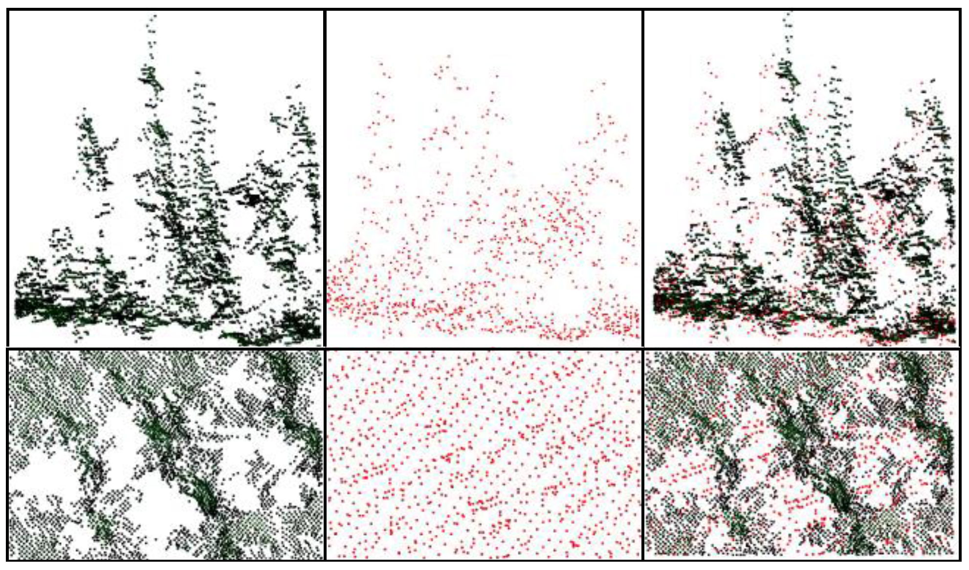
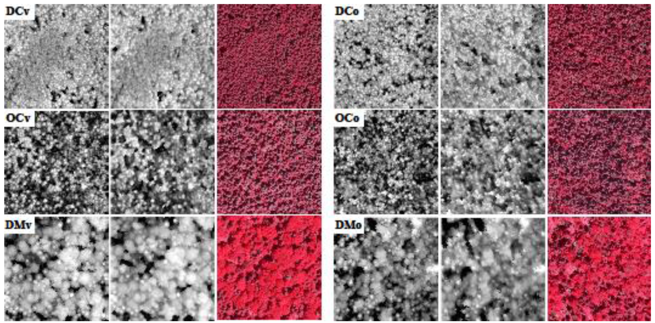
Figure 1 and Figure 2 show different renderings of the lidar and PPC data. In the first figure the lidar and photogrammetric points are presented from a virtual oblique view direction, revealing the content and structure of the point clouds for the dense conifer site viewed at a near vertical angle. We see that the point density of the PPC is higher than that of the lidar, but that the photogrammetric points sometimes occurred in dense clusters, leaving small gaps. The characteristic elongated and conical shape of the firs can be well perceived in the PPC, as well as in the lidar data, although with a lesser point density. The second figure shows the lidar and PPC-based canopy height models of the six sites. In each of these, the corresponding CHMs are visually strikingly similar. Individual tree crowns are easily visible as bright blobs in the PPC-based CHM also. However, they appear less well resolved in the DCo site in the PPC-based CHM, compared to the DCv site.

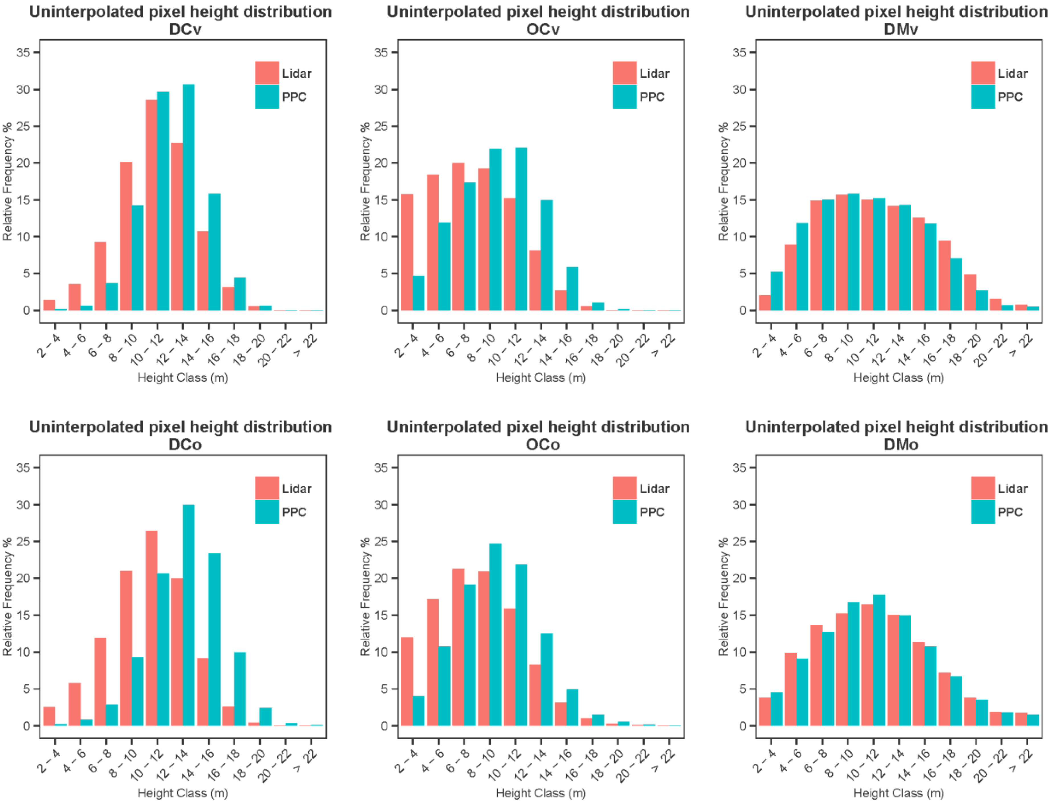
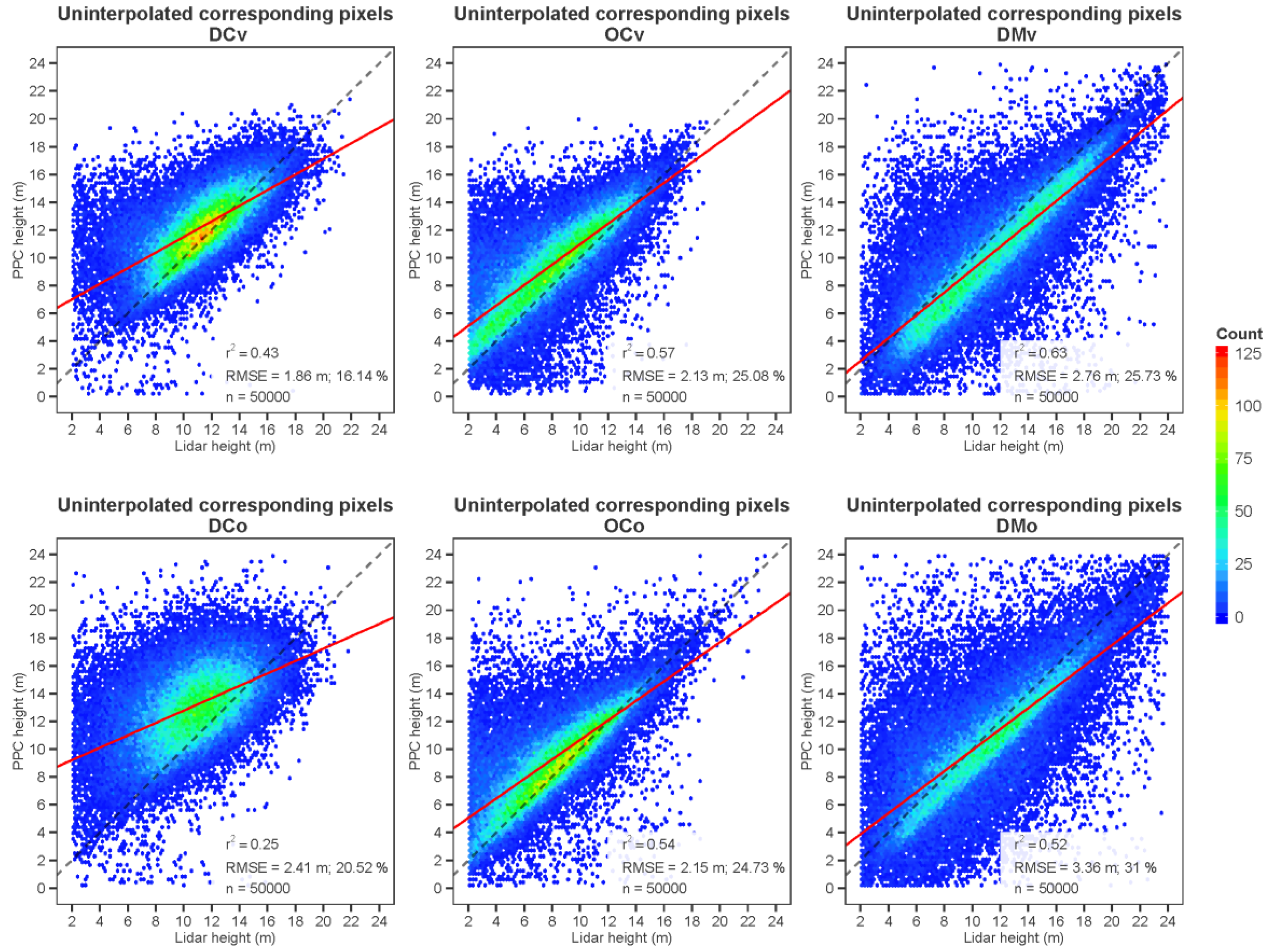
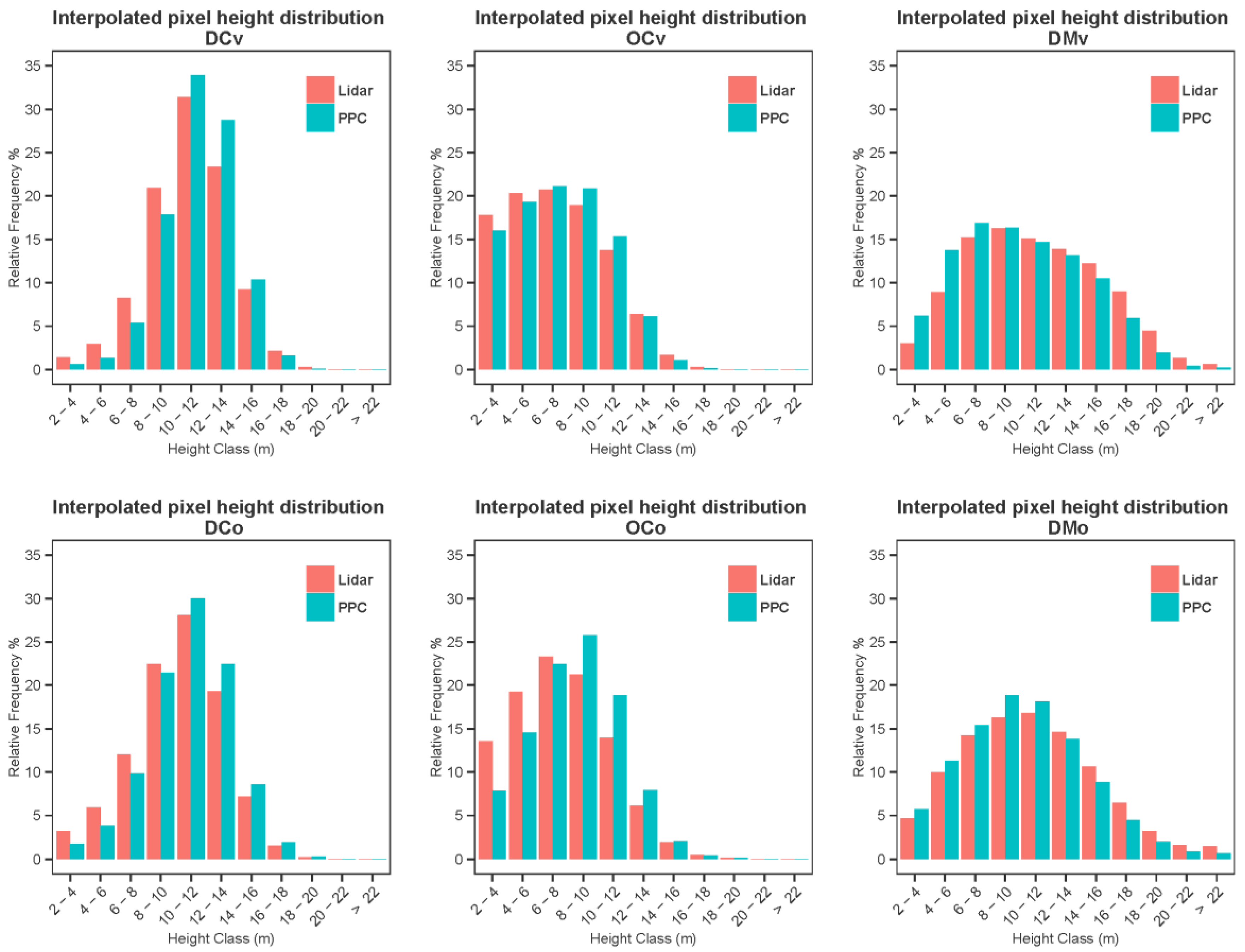
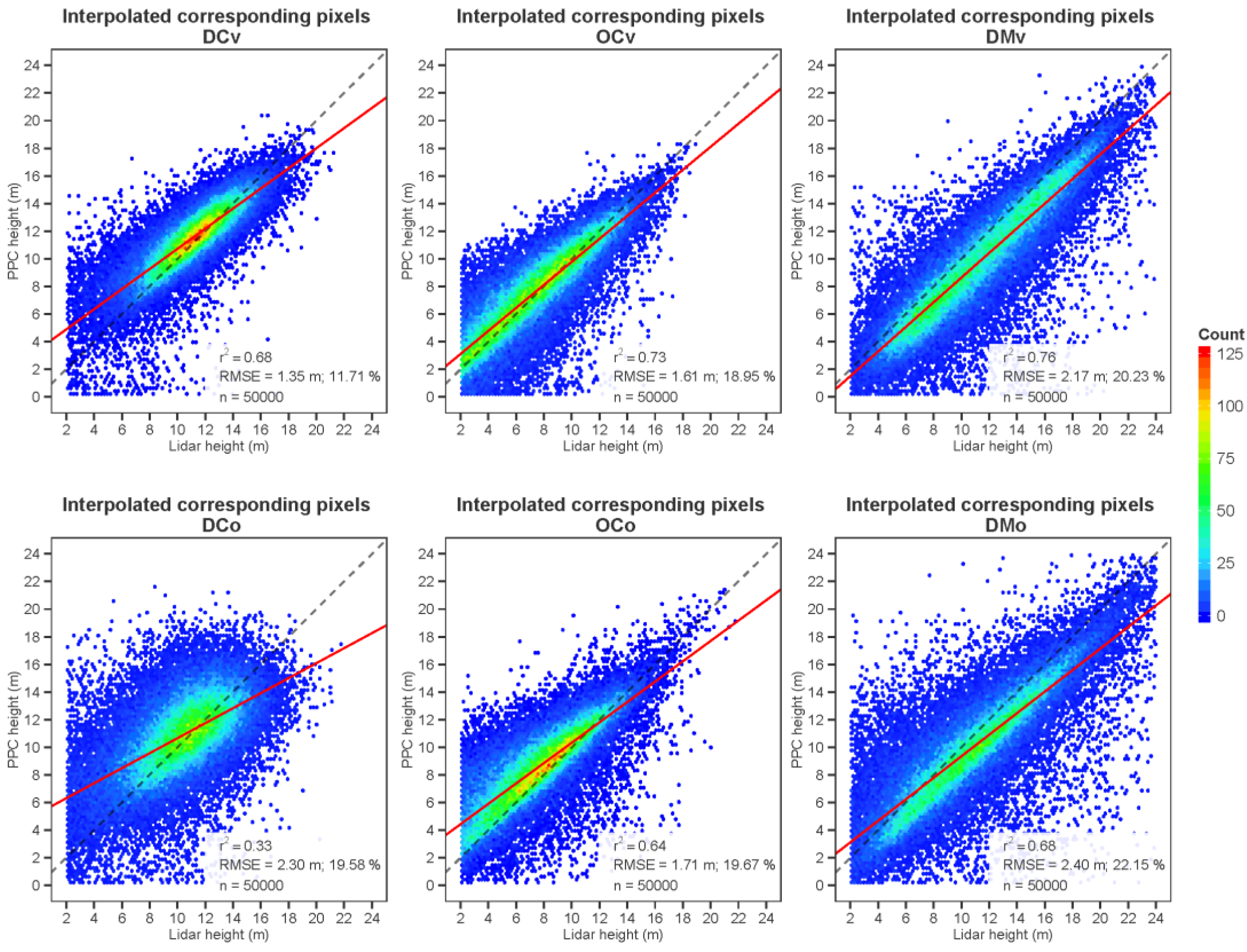
The corresponding relative histograms of lidar and photogrammetric point height at corresponding pixel locations are presented for the uninterpolated CHM (Figure 3) and interpolated CHM (Figure 4). As could be expected, the relative lidar frequencies of smaller point heights were greater in the more open sites as smaller trees and shrubs were visible between higher trees, and the dense even-age conifer sites having trees of similar sizes presented a more leptokurtic distribution. Disparities between the lidar and PPC distributions varied from very small in the case of dense mixed sites (viewed vertically or obliquely), to moderate, in the case of the dense conifer stands. In this latter case, low height relative frequencies were markedly underestimated, leading to an overestimation of the frequency of greater heights. This underestimation was stronger in the oblique view. Frequency differences were not as great in open conifer stands and the effect of obliquity was less pronounced in that case.

Figure 1. From left to right, virtual views of photogrammetric point clouds (dark colored points), lidar (red points) and both of a balsam fir stand (horizontal view in the first row, vertical view in the bottom row).

Figure 1. From left to right, virtual views of photogrammetric point clouds (dark colored points), lidar (red points) and both of a balsam fir stand (horizontal view in the first row, vertical view in the bottom row).

Figure 2. Lidar (left) and photogrammetric (PPC)-based (middle) canopy height models 250 m × 250 m excerpts (brightness proportional to height) with corresponding orthophoto (right) of the six sites. DC: dense conifers; OC: open conifers; DM: dense mixed woods; v: vertical; o: oblique.

Figure 2. Lidar (left) and photogrammetric (PPC)-based (middle) canopy height models 250 m × 250 m excerpts (brightness proportional to height) with corresponding orthophoto (right) of the six sites. DC: dense conifers; OC: open conifers; DM: dense mixed woods; v: vertical; o: oblique.

Figure 3. Relative point height distributions of lidar and photogrammetric points for corresponding locations of the uninterpolated canopy height models (CHMs).

Figure 3. Relative point height distributions of lidar and photogrammetric points for corresponding locations of the uninterpolated canopy height models (CHMs).

The points used to calculate the histograms of Figure 3 are those for which both a lidar and a photogrammetric point existed at a given pixel location. The spatial distribution of the photogrammetric points was much less uniform than that of the lidar points. In PPCs, we could often observe (e.g., Figure 1) dense clusters on visible sides of crowns, surrounded by voids (absence of points). Interpolating the lidar and photogrammetric points has evened the spatial distributions and filled the voids with predicted values, with the effect of diminishing the discrepancies between the lidar and PPC relative point height distributions (Figure 4). The most notable improvement brought about by interpolation is for dense conifers viewed obliquely. Moreover, the difference between the lidar and PPC distributions in the case of dense mixed sites was not sensibly improved by interpolation.

Figure 4. Relative point height distributions of lidar and photogrammetric points for corresponding locations of the interpolated CHMs.

Figure 4. Relative point height distributions of lidar and photogrammetric points for corresponding locations of the interpolated CHMs.

Figure 5 and Figure 6 present scatter plots of the relationships between lidar and photogrammetric heights based on the corresponding pixels of the uninterpolated and interpolated CHMs respectively, as well as the slope, coefficient of determination and RMSEs of these relationships. The worst correspondence was that of dense conifers viewed obliquely (r² of 0.25; RMSE = 2.41 m; a strong departure from the 1:1 slope). The best relationship was seen for dense mixed woods viewed vertically. The slope was in this case much closer to the 1:1 line, and the r² much higher at 0.63. The absolute RMSE was somewhat high, but this was likely due to the presence of a greater range in height (up to 24 m). Oblique viewing worsens the correspondence in all case, but obliquity has less of an effect in the case of open conifers.

As evidenced by Figure 6, interpolation markedly improved the correspondence between lidar and photogrammetric heights. The improvement is important for all sites except the dense conifer site viewed obliquely where the r² remains low, at 0.33.

Figure 5. Scatterplots of the height correspondence between lidar and photogrammetric uninterpolated CHMs (red line represents the slope of the relationships and dashed line represents the 1:1 relationship).

Figure 5. Scatterplots of the height correspondence between lidar and photogrammetric uninterpolated CHMs (red line represents the slope of the relationships and dashed line represents the 1:1 relationship).

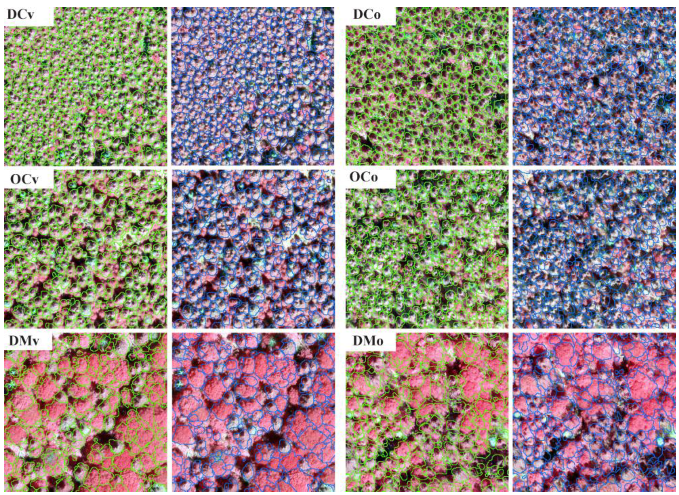
The individual crowns automatically extracted from the lidar and PPC-based CHMs respectively are presented in Figure 7. Single tree extraction was possible on the photogrammetric CHMs, but did not perform as well as in the lidar case. In several cases, for example, single tree crowns extracted from the lidar were merged in the photogrammetric delineations, as evidenced in Table 6. The number of detected crowns in the PPC-based CHMs were somewhat lower (11.7%–19.9% less) than what was found in their lidar counterpart, except in the case of the DCo site where 1.3% more crowns were found in the PPC. The underestimation was always less in the case of the oblique views.

Table 6. Number of delineated trees based respectively on the lidar and PPC-based CHMs, and relative difference (PPC minus lidar) in %.

	DCv	DCo	OCv	OCo	DMv	DMo
Lidar	4773	4769	2893	3021	8803	8776
PPC	3974	4829	2316	2486	7055	7751
Difference (%)	−16.7	1.3	−19.9	−17.7	−19.9	−11.7

DC: dense conifers; OC: open conifers; DM: dense mixed woods; v: vertical; o: oblique.

Table 6. Number of delineated trees based respectively on the lidar and PPC-based CHMs, and relative difference (PPC minus lidar) in %.

	DCv	DCo	OCv	OCo	DMv	DMo
Lidar	4773	4769	2893	3021	8803	8776
PPC	3974	4829	2316	2486	7055	7751
Difference (%)	−16.7	1.3	−19.9	−17.7	−19.9	−11.7

DC: dense conifers; OC: open conifers; DM: dense mixed woods; v: vertical; o: oblique.

Figure 6. Scatterplots of the height correspondence between lidar and photogrammetric interpolated CHMs (red line represents the slope of the relationships and dashed line represents the 1:1 relationship).

Figure 6. Scatterplots of the height correspondence between lidar and photogrammetric interpolated CHMs (red line represents the slope of the relationships and dashed line represents the 1:1 relationship).

Figure 7. Crown delineation results for lidar (green outlines) and PPC-based CHMs (blue outlines). All image excerpts are 65 m × 65 m (DC: dense conifers, OC: open conifers, DM: dense mixed woods, v: vertical, o: oblique).

Figure 7. Crown delineation results for lidar (green outlines) and PPC-based CHMs (blue outlines). All image excerpts are 65 m × 65 m (DC: dense conifers, OC: open conifers, DM: dense mixed woods, v: vertical, o: oblique).

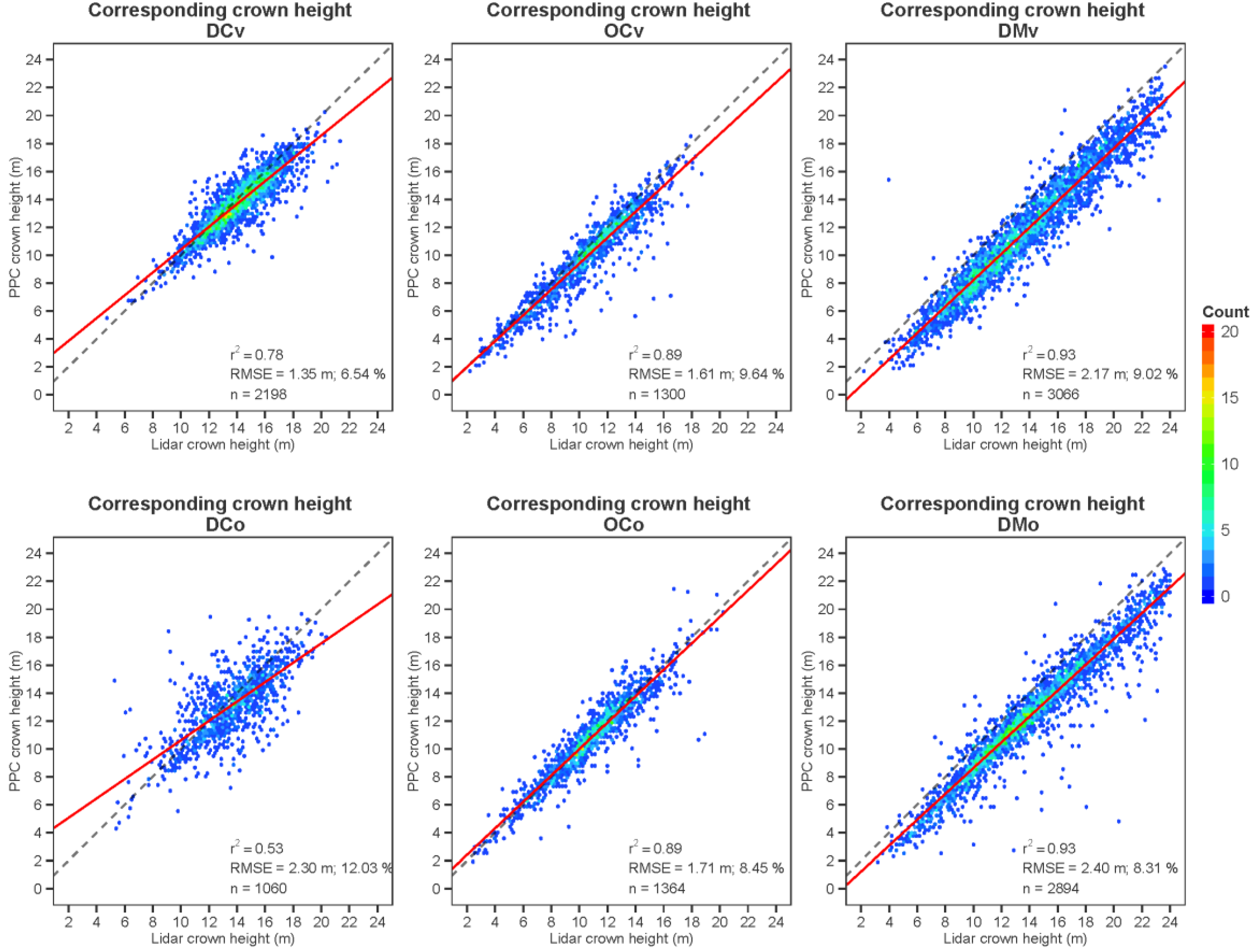
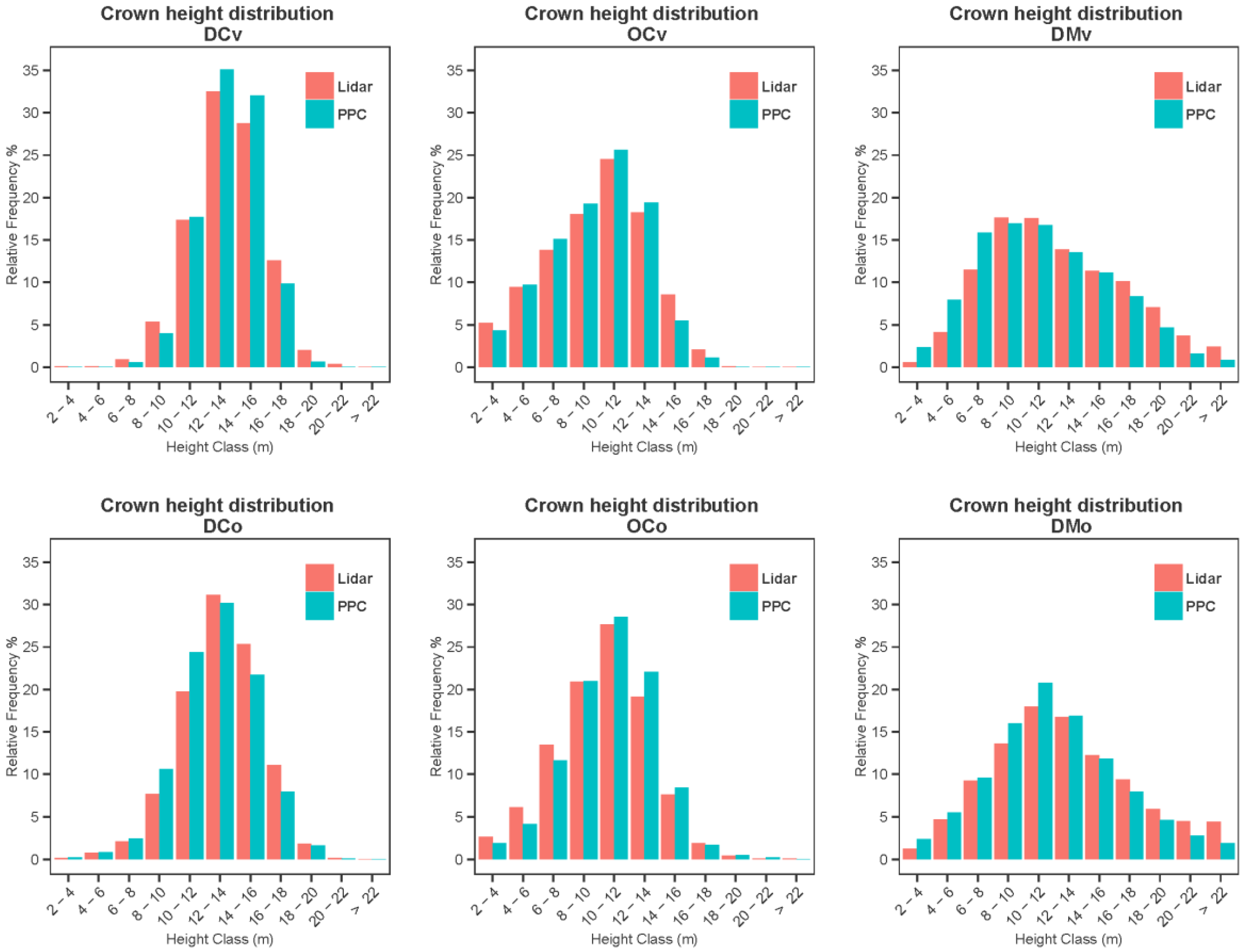
Before proceeding to the comparison of the lidar and PPC-based crown heights, we assessed the accuracy of the former, considered as the reference, by comparing them to heights measured in the field. A general average r² of 0.93 and RMSE of 1.29 m with a bias of −0.98 m were obtained over the 431 control trees (all species). These values were respectively 0.93, 1.31 m and −1.12 m for balsam firs, 0.93, 1.10 m and 1.62 m for spruces, and 0.98, 0.32 m and −0.26 m for deciduous trees. Moreover, the discrepancies between lidar and PPC-based relative tree height frequencies (Figure 8) were similar to those observed at point level in the interpolated CHMs, but modest improvements appeared for open conifers viewed obliquely (OCo). However, the height correspondence between lidar and PPC crowns was much greater at tree level (Figure 9), than for individual points of the CHMs (Figure 5 and Figure 6), with r² ranging from 0.53 to 0.93, and RMSEs as low as 1.35 m. In the case of open conifers and dense mixed forests, obliquity did not significantly modify the performance of height retrieval. The dense mixed site imaged obliquely presented the greatest level of error, with a RMSE of 2.40 m.

Figure 8. Relative tree height distributions derived respectively from lidar and PPCs.

Figure 8. Relative tree height distributions derived respectively from lidar and PPCs.

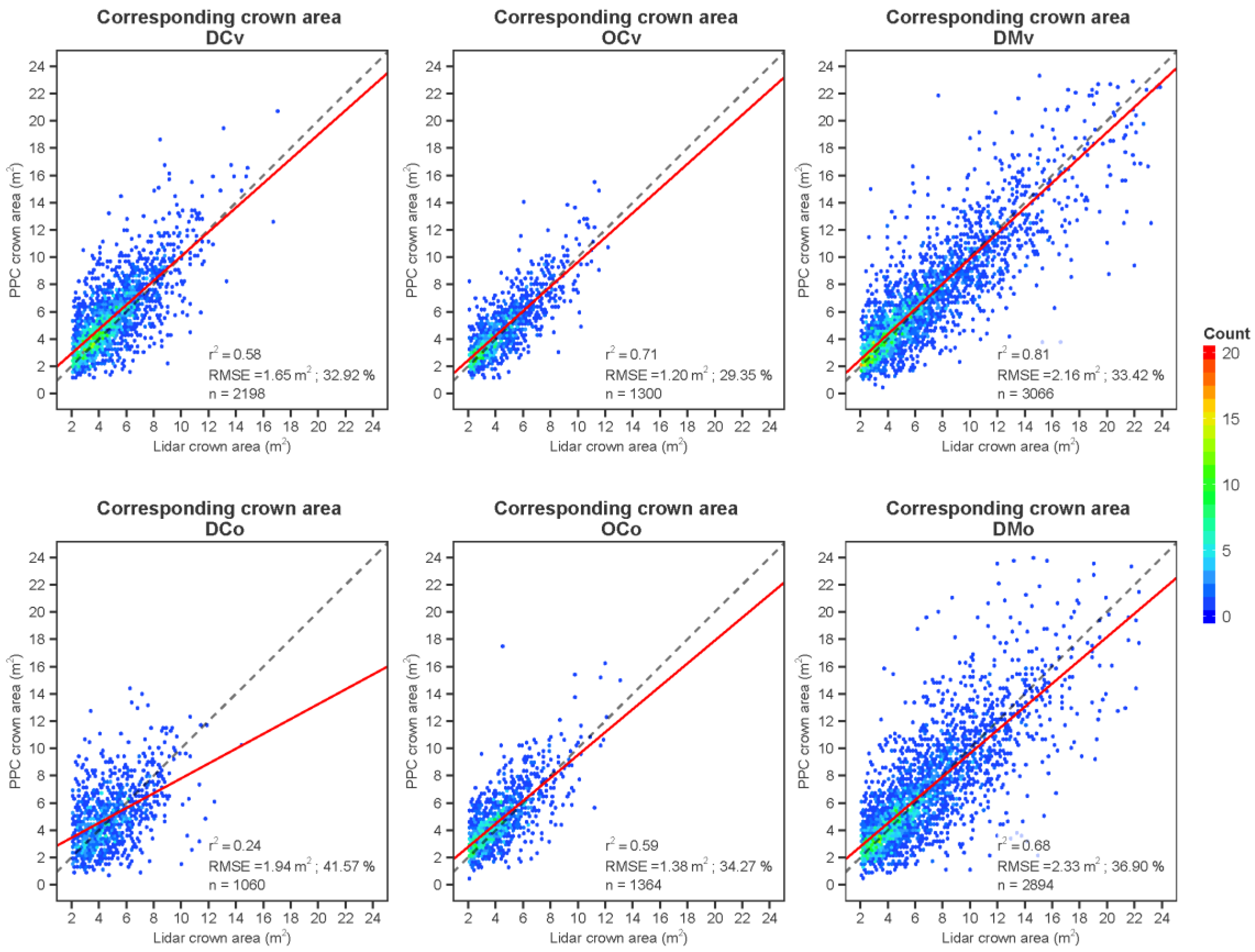
The correspondence of the delineated areas of crowns was much less than for height (Figure 10). The best relationship based on the coefficient of determination was obtained for the dense mixed woods viewed vertically (r² of 0.81 and a RMSE of 2.16 m²). The slope of the relationships was quite close to 1, except for tree height in the case of the DCo site.

Figure 9. Scatterplots of the lidar and PPC-based tree heights (red line represents the slope of the relationships and dashed line represents the 1:1 relationship).

Figure 9. Scatterplots of the lidar and PPC-based tree heights (red line represents the slope of the relationships and dashed line represents the 1:1 relationship).

The random forest classification results for deciduous, fir and spruce trees are presented in Table 7. In this table, OOB designates the out of bag error of the random forest classification from training dataset. The overall accuracy, producer’s and user’s accuracy and kappa coefficient results were calculated by classifying the validation dataset. Overall classification accuracies varied from 79.0% to 89.0%. The PPC-based classifications involving both 3D and intensity metrics were systematically the best, but were just marginally superior to those obtained from lidar. The lidar 3D metrics were superior to their photogrammetric counterpart, but the addition of the intensity metrics provided a strong increase of accuracy in the case of the photo-based results, while not causing any sensible improvement for lidar. In general, producer’s and user’s classification accuracies were lower for the spruce class. Obliquity did not have a strong effect on the species identification results. Training and applying the random forest classifier on the crowns of the two sites taken as a whole did not affect the results despite the variations that may exist in the 3D point clouds or photographic intensity characteristics.

The usefulness of the different metrics evaluated through the mean decrease in accuracy, and mean decrease of the Gini index they bring about, is presented in Table 8. It shows that the curve-based metrics, indicative of the crown 3D shape, and the area over height ratio (proportion), came out first for both lidar (with or without intensity) and 3D-only PPCs. However, when the full PPC data was used, i.e., including multispectral image brightness, the two most useful variables were intensity based (R_std and NIR_mean), outperforming the curved-based variables.

Figure 10. Scatterplots of the lidar and PPC-based tree crown areas (red line represents the slope of the relationships and dashed line represents the 1:1 relationship).

Figure 10. Scatterplots of the lidar and PPC-based tree crown areas (red line represents the slope of the relationships and dashed line represents the 1:1 relationship).

Table 7. Species classification results from lidar and PPC data.

Variables Set	OOB	Overall Accuracy	Kappa	Producer’s/User’s Accuracy			n Variables
				Deciduous	Fir	Spruce
DMv
Lidar 3D	19	83	62	79/76	91/85	37/88	23
Lidar 3D + intensity	18	86	68	84/86	95/86	32/86	29
PPC 3D	19	79	55	61/71	89/80	54/81	15
PPC 3D + spectral	9	89	78	88/92	95/89	63/83	21
DMo
Lidar 3D	17	85	65	77/84	95/85	21/75	24
Lidar 3D + intensity	15	86	67	79/84	95/86	29/80	30
PPC 3D	18	79	54	60/86	94/79	29/56	14
PPC 3D + spectral	12	87	72	82./91	96/86	35/67	21
DMv + DMo
Lidar 3D	17	86	67	77/82	94.64/87	36/86	24
Lidar 3D + intensity	17	86	68	82/83	93.87/88	36/80	30
PPC 3D	18	79	55	65/74	90.00/82	41/65	14
PPC 3D + spectral	11	89	76	87/90	94.80/90	54/73	21

n is the number of variables, OOB is the out of bag error of the random forest classification from training dataset.

Table 7. Species classification results from lidar and PPC data.

Variables Set	OOB	Overall Accuracy	Kappa	Producer’s/User’s Accuracy			n Variables
				Deciduous	Fir	Spruce
DMv
Lidar 3D	19	83	62	79/76	91/85	37/88	23
Lidar 3D + intensity	18	86	68	84/86	95/86	32/86	29
PPC 3D	19	79	55	61/71	89/80	54/81	15
PPC 3D + spectral	9	89	78	88/92	95/89	63/83	21
DMo
Lidar 3D	17	85	65	77/84	95/85	21/75	24
Lidar 3D + intensity	15	86	67	79/84	95/86	29/80	30
PPC 3D	18	79	54	60/86	94/79	29/56	14
PPC 3D + spectral	12	87	72	82./91	96/86	35/67	21
DMv + DMo
Lidar 3D	17	86	67	77/82	94.64/87	36/86	24
Lidar 3D + intensity	17	86	68	82/83	93.87/88	36/80	30
PPC 3D	18	79	55	65/74	90.00/82	41/65	14
PPC 3D + spectral	11	89	76	87/90	94.80/90	54/73	21

n is the number of variables, OOB is the out of bag error of the random forest classification from training dataset.

Table 8. Mean decrease in accuracy, and mean decrease of the Gini index associated to the metrics for each of the classifications.

	Mean Decrease Accuracy	Mean Decrease Gini		Mean Decrease Accuracy	Mean Decrease Gini
Lidar 3D			PPC 3D
Curve_75	24.49	36.56	Curve_75	23.17	32.39
Curve_50	16.05	23.24	Curve_50	21.52	29.58
Curve_all	13.52	23.22	Area/H	17.78	28.08
Area/H	12.08	26.46	Hull_50	16.97	26.86
Md1_max1	11.86	26.44	Hull_75	16.22	23.47
Hull_75	10.83	20.34	Rcurve_50	14.83	25.07
Hull_50	10.61	24.28	Rcurve_all	14.50	25.60
Rcurve_50	8.33	14.32	Pt_75-100	13.62	24.49
Hull_all	8.06	18.59	Pt_50-75	12.94	22.74
Pt_50–75	7.94	17.93	Rcurve_75	11.45	15.07
Lidar 3D + intensity			PPC 3D + spectral
Curve_75	16.60	27.98	Std_r	29.58	35.24
Curve_50	12.26	20.03	Mean_nir	26.89	39.49
Curve_all	12.25	21.69	Curve_75	15.00	24.37
Area/H	9.77	22.26	Ndvi	14.27	30.32
Md1_max1	9.75	20.86	Curve_50	12.22	25.58
Hull_75	9.38	20.29	Cv_ir	10.89	22.95
Hull_50	8.81	19.75	Rcurve_all	9.74	24.36
Mn1_max1	7.36	19.13	Area/H	8.35	20.49
Hull_all	6.97	15.62	Rcurve_50	8.32	21.69
Mn1_maxA	6.95	16.05	Hull_all	5.42	18.71

Table 8. Mean decrease in accuracy, and mean decrease of the Gini index associated to the metrics for each of the classifications.

	Mean Decrease Accuracy	Mean Decrease Gini		Mean Decrease Accuracy	Mean Decrease Gini
Lidar 3D			PPC 3D
Curve_75	24.49	36.56	Curve_75	23.17	32.39
Curve_50	16.05	23.24	Curve_50	21.52	29.58
Curve_all	13.52	23.22	Area/H	17.78	28.08
Area/H	12.08	26.46	Hull_50	16.97	26.86
Md1_max1	11.86	26.44	Hull_75	16.22	23.47
Hull_75	10.83	20.34	Rcurve_50	14.83	25.07
Hull_50	10.61	24.28	Rcurve_all	14.50	25.60
Rcurve_50	8.33	14.32	Pt_75-100	13.62	24.49
Hull_all	8.06	18.59	Pt_50-75	12.94	22.74
Pt_50–75	7.94	17.93	Rcurve_75	11.45	15.07
Lidar 3D + intensity			PPC 3D + spectral
Curve_75	16.60	27.98	Std_r	29.58	35.24
Curve_50	12.26	20.03	Mean_nir	26.89	39.49
Curve_all	12.25	21.69	Curve_75	15.00	24.37
Area/H	9.77	22.26	Ndvi	14.27	30.32
Md1_max1	9.75	20.86	Curve_50	12.22	25.58
Hull_75	9.38	20.29	Cv_ir	10.89	22.95
Hull_50	8.81	19.75	Rcurve_all	9.74	24.36
Mn1_max1	7.36	19.13	Area/H	8.35	20.49
Hull_all	6.97	15.62	Rcurve_50	8.32	21.69
Mn1_maxA	6.95	16.05	Hull_all	5.42	18.71

5. Discussion

While previous studies on the characterization of forest structure or composition have compared only the end results obtained from airborne lidar and photogrammetric data [39,42,43], we have studied the difference between these two types of data over the full analysis workflow, from raw point cloud characteristics to classification results. This allowed a more complete understanding of the discrepancies and gave us the capacity to understand the effects of discrepancies at each processing level. We here outline the main differences between lidar and PPC-based results, at these different levels, and provide contextualized explanations.

Airborne lidar and aerial photos differ in their acquisition geometry. The maximum scan angle of lidar is commonly set to about 15 degrees from nadir. This can be contrasted with the much wider maximum lateral view angle of airborne photography (48 degrees in the case of the UltraCam). Although the maximum azimuthal view angle (along the flight axis) is less, and view angle problems can be alleviated in this direction by increasing the forward overlap of photographs at no cost, reducing these problems in the lateral direction is only possible by decreasing the distance between the flight lines, at relatively high cost. What is more, a photogrammetric point is generated for a given XYZ location only when this location is visible from at least two viewpoints. For this reason, the overall visibility of the trees is much less in the photogrammetric case than it is in the lidar case. This effect is more pronounced for trees having an elongated shape (e.g., boreal conifer trees) than for those with a more spherical crown, such as boreal deciduous trees, because seeing within the deep troughs between close-by trees is difficult in the case of conifers. Thus, view obliquity has lesser effects in dense mixed woods (and in theory also in pure deciduous forests). This effect appears clearly in Figure 3 where the histograms of the uninterpolated pixel values are quite similar between lidar and PPCs for the DMv and DMo sites. Other researchers noted similar effects [10,36]. Openness of the canopy decreases the effect of obliquity (Figure 3) because inter-tree occlusions are less frequent. Interpolation improves the correspondence between the two types of data, and decreases the effect of obliquity, because it fills data voids according to the immediate 3D context with values that often seem to concord between lidar and PPCs. However, a full explanation of this improvement would necessitate a deeper investigation, which is outside the scope of the present study.

The correspondence between individual tree heights (Figure 8 and Figure 9) is markedly higher than the in the pixel-based comparison, a result that is not surprising considering that the tree apices are viewed much more easily than their low sides in the photogrammetric case. The overall number of detected trees is lower in the case of the photogrammetric results because some crowns are not resolved in the PPC-based CHM. One of the main causes of this is that occlusion of the low sides or far sides of trees sometimes leaves data gaps between visible apices that are then bridged by the interpolation. Also, because matching is performed using, among other things, small matching windows (e.g., having a size of 7 × 7 pixels), the resulting photogrammetric point cloud is expected to be somewhat smoother than corresponding lidar point clouds. The tree delineation algorithm, sensing no significant inter-tree valley in this case, will merge neighboring crowns. Nevertheless, the relative frequencies per height class were very similar (Figure 8), making the characterization of the height distribution quite accurate. The PPC height of single trees was also very accurate, being highly correlated to that of lidar, which itself was demonstrated to be close to the ground truth values. However, the loss of 3D resolution in the PPC-based CHM caused by the smoothing effect and the loss of points due to occlusions created much higher discrepancies in the case of crown area. Not being always able to reconstruct the full 3D shape of the trees in the PPC case resulted in much less reliable crown outline boundaries, with a logical impact on the crown area estimation.

Notwithstanding the abovementioned limitations of the PPCs, the tree species classification results for deciduous, fir and spruce trees were superior for this data type when using all the available 3D and intensity metrics. As could be expected, the 3D metrics of lidar outperformed those of PPCs, albeit not markedly, for reasons related to the previously highlighted shortcomings of the photogrammetric data. However, the rich multispectral contents of the PPCs did compensate for its lower 3D information contents. Lidar intensity did not improve the classification results by much, probably because the lidar 3D information itself was very rich, making the single wavelength intensity information content largely redundant. Although the vertical and oblique sites (DMv and DMo) were extracted from respectively close areas, far away from the aerial image centers, and although they fell on different images, it appears that the photo intensity response was nevertheless quite similar. This was demonstrated by the DMv + DMo classification in Table 7 where classification accuracy did not clearly decrease even though the sun-target-sensor geometry was quite different between the sites. Radiometric normalization however remains recommendable when using image intensity metrics, particularly if the photos were acquired over different days.

We recognize that the present study has certain limitations. First, the 3D coregistration between the lidar and photogrammetric models was not highly accurate. In these dense forests, the ground is often invisible, leaving few areas where accurate ground control points extracted from the lidar DTM can be associated to photo pixels. This logically affects the CHM-based correspondences more than the ITC based results. Using more accurate coregistration techniques, such as point cloud registration [58], we suspect that the lidar-PPC discrepancies of Figure 3 and Figure 4 would somewhat diminish, and the regression lines of the pixel and crown height relationships would move closer to the 1:1 lines.

Secondly, the results on crown height concern corresponding lidar-PPC crowns that were automatically selected, and the results on species were obtained from crowns selected by the photo-interpreter with a possible involuntary subjective bias occurring during the selection process. This likely leaves out many erroneously delineated PPC crowns from which incorrect 3D and intensity metrics values would be extracted and introduced into the classification, leading to lower identification accuracies. A full assessment of the comparative performances of lidar and photogrammetry in this regard would require comparisons with ground truthed crown delineations, a very labor intensive and costly endeavor. Furthermore, a wider set of lidar and PPC-based metrics should be tested, and a larger number of lidar and aerial images reflecting various conditions of forest structure, composition (with a greater number of species), topography and acquisition geometries should be investigated. However, the six study sites in our experiments covered areas ranging from 3 to 12 ha. In particular, classification tests were conducted on two 12 ha sites, which is likely to confer robustness to the results. We therefore think that the results presented in this study are highly indicative of the potential of forest structure and composition characterization based on photogrammetric point clouds analyzed with an individual tree crown approach.

6. Conclusions

The results of this study lead us to conclude that the characterization of the tree height distribution and general species composition of boreal forests based on ITC analysis of photogrammetric point clouds can be achieved with an accuracy similar to that obtained from airborne lidar data. Despite occlusion effects in the PPCs that are apparent at the level of points or pixels, crown-based results do not differ markedly. However, the estimation of crown areas showed much higher discrepancies between lidar and PPC-based results. We also found that the quality of the ITC-based results, in terms of height estimation or species identification, was rather uniform across the image space, i.e., not strongly affected by photographic viewing geometry. Finally, the PPC 3D classification metrics provided important species identification data which, when combined to multispectral image intensities, led to higher classification accuracies than the lidar 3D and intensity metrics.

Aerial photo acquisition remains significantly less expensive than that of airborne lidar due to higher flying altitudes, wider view angles and greater flight speeds. For this reason, provided that an accurate DTM is available, from lidar or other sources, the general characterization of the height structure and species composition based on photogrammetric point clouds becomes possible. PPC-based results could be further improved by reducing the effects of occlusions in the stereo models, either by using a more intelligent approach for height interpolation to fill the PPC data gaps, or by increasing the lateral overlap of aerial images. This latter solution would entail higher acquisition costs due to the greater number of required flight lines, but could be configured to be still less costly than lidar. Furthermore, the operational deployment of such technology over large territories creates the obligation to tackle the issue of variable sun elevations or atmospheric conditions which affect image intensities in a complex way, thus requiring the implementation of intensity normalization strategies. Notwithstanding these processing complications, forest managers and scientist will certainly benefit from the data gathering capacities offered by individual tree crown analysis of photogrammetric point clouds.