
Aboveground Biomass Estimation Using Structure from Motion Approach with Aerial Photographs in a Seasonal Tropical Forest

Abstract
:
1. Introduction
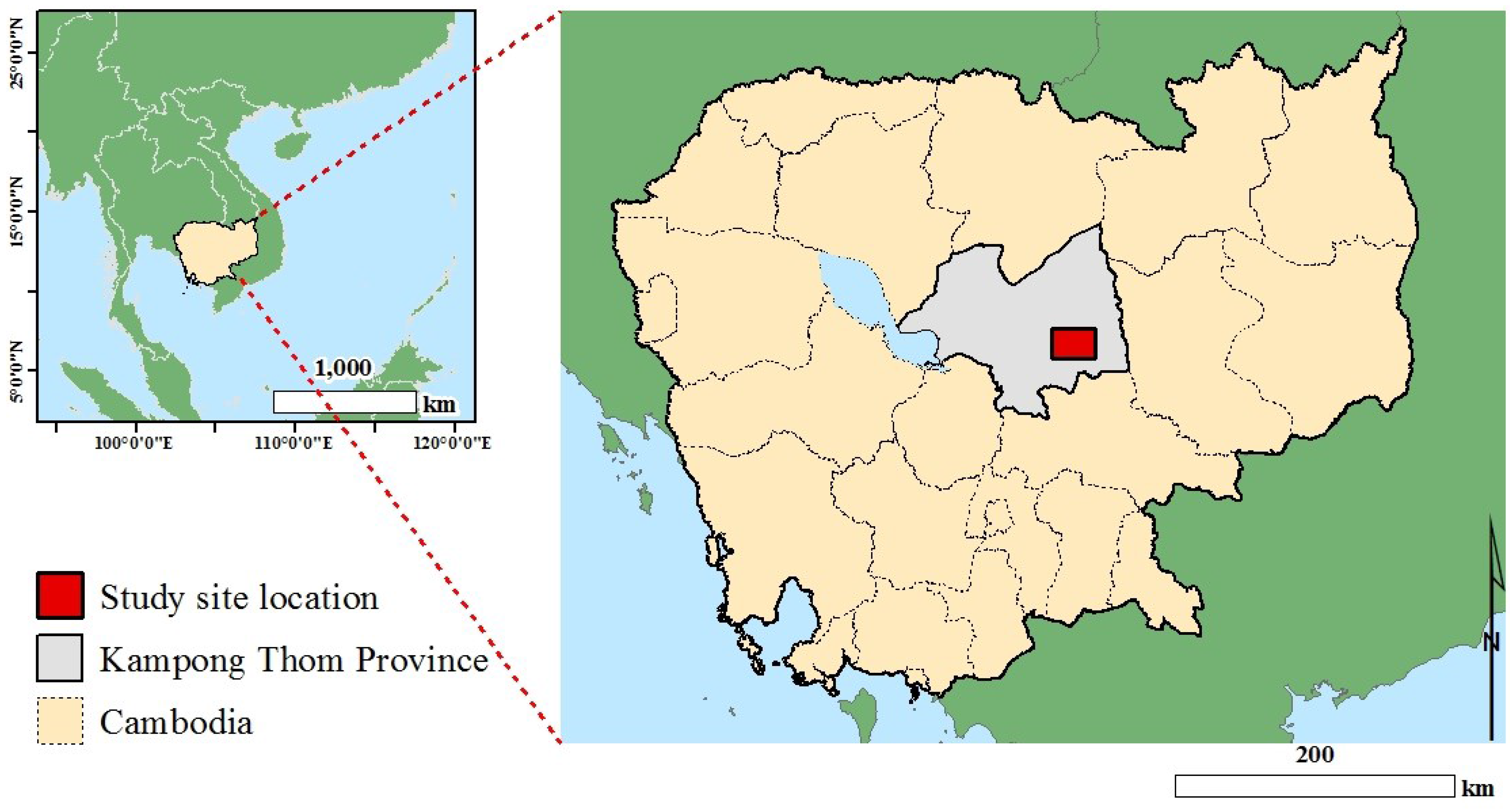
2. Study Area

3. Field Measurements

| Forest type | Count | AGB (Mg/ha) | |||
|---|---|---|---|---|---|
| Min | Mean | Max | SD | ||
| Evergreen | 10 | 176 | 294 | 398 | 65 |
| Degraded evergreen | 4 | 96 | 132 | 176 | 31 |
| Deciduous | 8 | 38 | 98 | 150 | 40 |
| Regrowth | 8 | 22 | 42 | 90 | 21 |
4. Remote Sensing Data
| Flight Conditions | |
|---|---|
| Flight altitude (above-ground) | 500 m |
| Flying Speed | 25 m/s |
| Acquisition date | 18–21 January, 2012 |
| Aerial Photograph data acquisition | |
| Instruments | DALSA Sensor + 60.5 Mp Image Sensor 8984 (H) x 6732 (V) Full Frame CCD Color Image Sensor with Rodenstock HR Digaron-W 50 mm f/4 lens. |
| Focal length | 51.2499 mm |
| Scale | 8984 × 6732 pixels |
| Pixel size | 6 μm |
| Ground resolution | 7 cm |
| Average density of point cloud | 22 points/m2 |
| Airborne LiDAR data acquisition | |
| Instruments | Optech ALTM 3100 from Optech, Inc. |
| Pulse repetition frequency | 100 kHz |
| Scan frequency | 53 Hz |
| Foot print | 0.125 m |
| Wave length | 1064 nm |
| Range of view angles | 20° |
| Average density of first returns | 26 pulse/m2 |
5. Methods
5.1. Processing of Airborne LiDAR data

5.2. Processing of Aerial Photographs
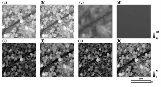
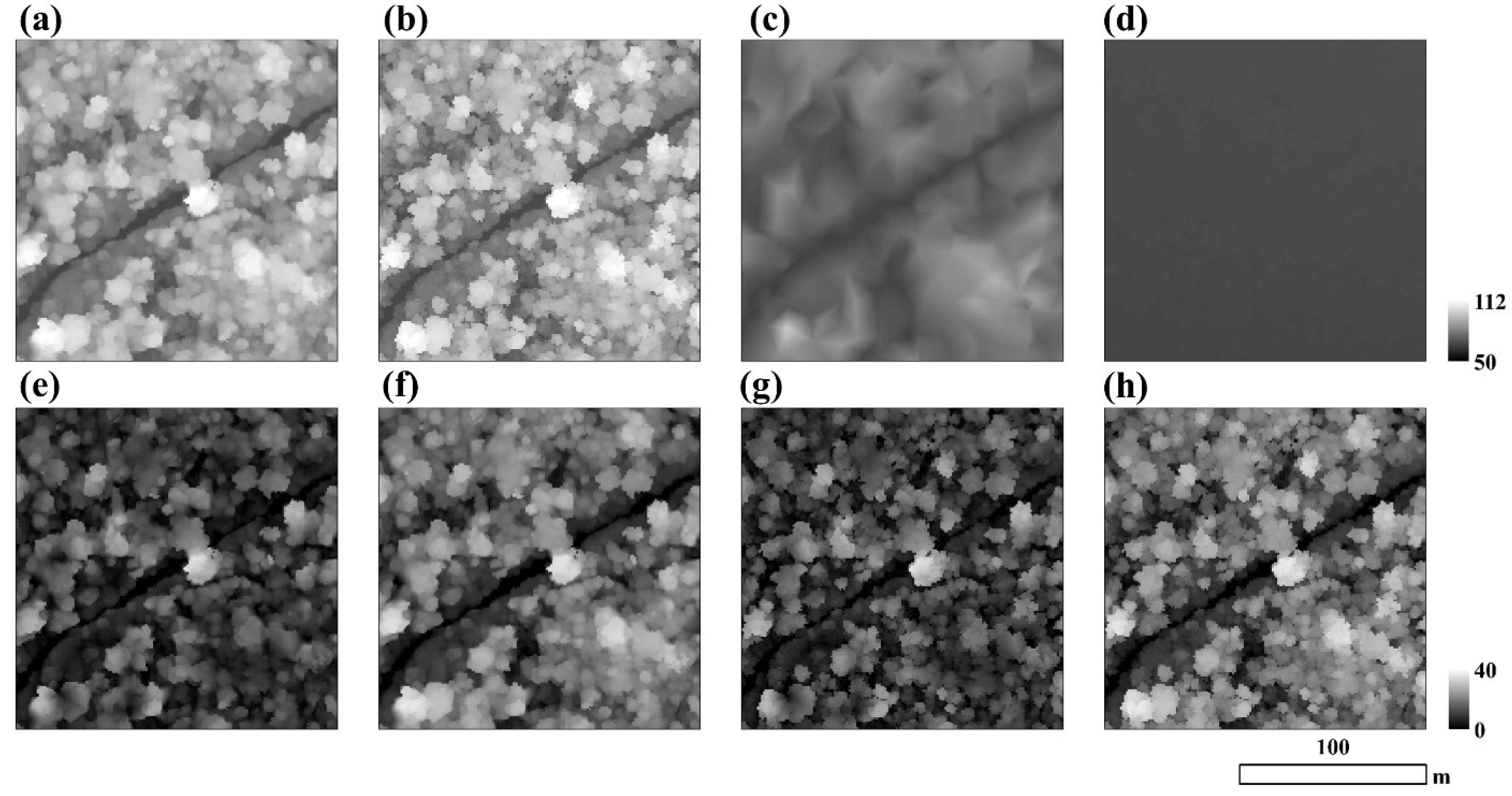
5.3. Calculation of CHM and CHM-Derived Variables
5.4. Statistical Analysis
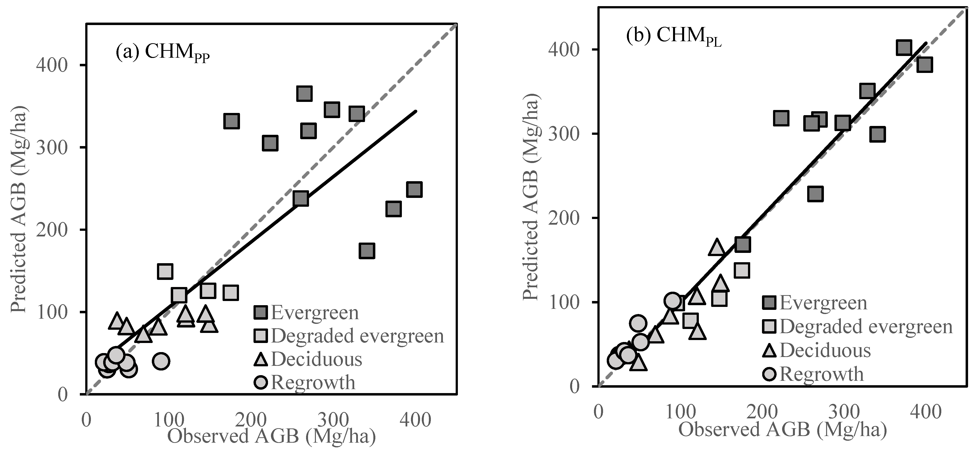
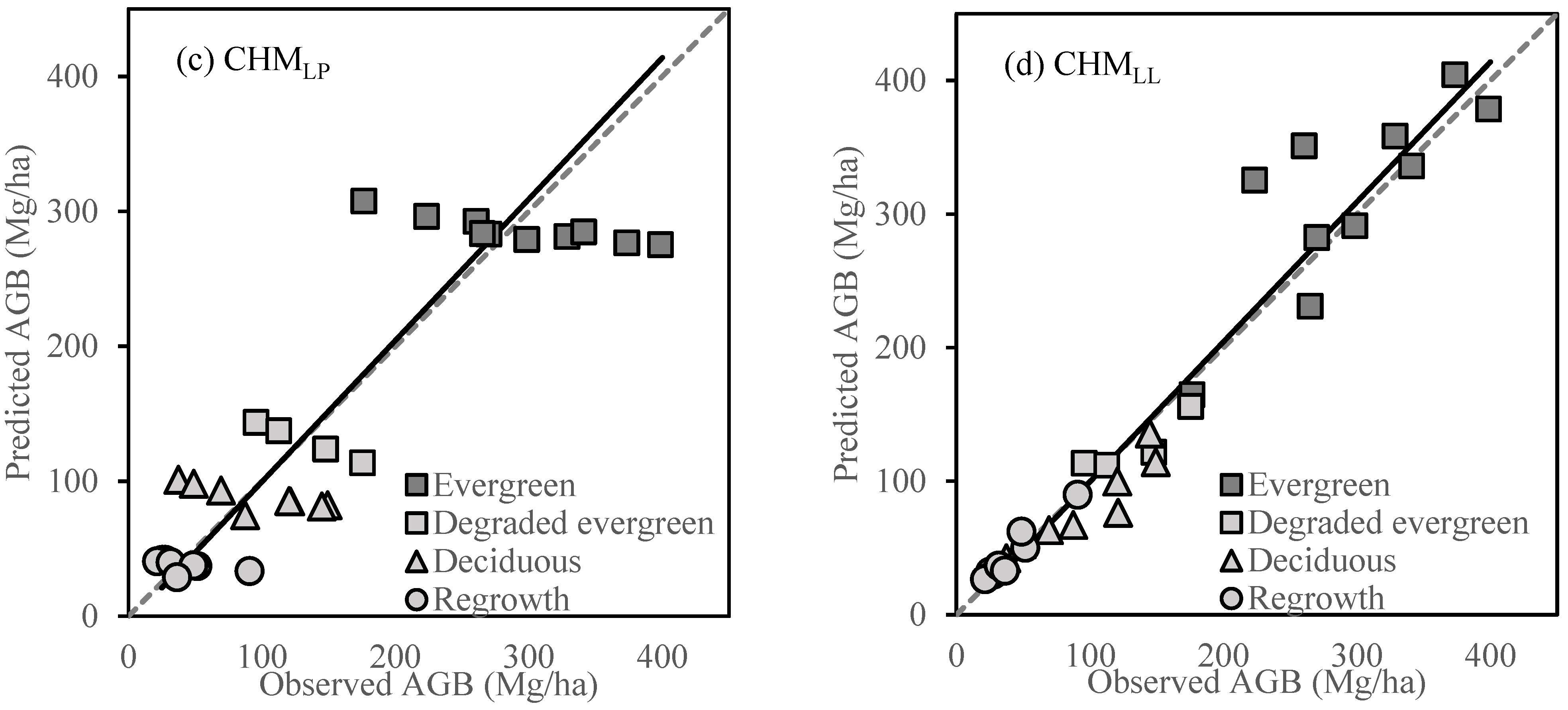
6. Results
| Variables | RMSE (Mg/ha) | R2 | Adjusted R2 | |
|---|---|---|---|---|
| CHMPP | H50 | 109.91 | 0.20 | 0.17 |
| H100 | 103.06 | 0.24 | 0.22 | |
| Hmean | 98.82 | 0.31 | 0.28 | |
| D | 113.99 | 0.10 | 0.06 | |
| H50 + D | 97.97 | 0.30 | 0.25 | |
| H100 + D | 93.68 | 0.36 | 0.31 | |
| Hmean + D | 89.54 | 0.41 | 0.36 | |
| H50 + Ftype | 56.81 | 0.75 | 0.72 | |
| H100 + Ftype | 68.24 | 0.66 | 0.61 | |
| Hmean + Ftype | 63.48 | 0.70 | 0.66 | |
| D + Ftype | 51.79 | 0.79 | 0.76 | |
| H50 + D + Ftype | 56.22 | 0.76 | 0.71 | |
| H100 + D + Ftype | 67.06 | 0.67 | 0.61 | |
| Hmean + D + Ftype | 62.12 | 0.71 | 0.65 | |
| CHMPL | H50 | 32.55 | 0.92 | 0.92 |
| H100 | 55.29 | 0.79 | 0.78 | |
| Hmean | 31.30 | 0.93 | 0.93 | |
| D | 114.42 | 0.10 | 0.07 | |
| H50 + D | 35.92 | 0.91 | 0.90 | |
| H100 + D | 55.16 | 0.79 | 0.78 | |
| Hmean + D | 33.36 | 0.93 | 0.92 | |
| H50 + Ftype | 30.31 | 0.93 | 0.92 | |
| H100 + Ftype | 46.10 | 0.84 | 0.81 | |
| Hmean + Ftype | 28.47 | 0.94 | 0.93 | |
| D + Ftype | 49.02 | 0.82 | 0.79 | |
| H50 + D + Ftype | 31.34 | 0.92 | 0.91 | |
| H100 + D + Ftype | 43.54 | 0.86 | 0.83 | |
| Hmean + D + Ftype | 29.47 | 0.93 | 0.92 |
| Variables | RMSE (Mg/ha) | R2 | Adjusted R2 | |
|---|---|---|---|---|
| CHMLP | H50 | 118.28 | 0.14 | 0.11 |
| H100 | 106.72 | 0.19 | 0.16 | |
| Hmean | 104.53 | 0.25 | 0.22 | |
| D | 124.23 | 0.05 | 0.02 | |
| H50 + D | 118.31 | 0.13 | 0.07 | |
| H100 + D | 107.73 | 0.17 | 0.11 | |
| Hmean + D | 104.77 | 0.24 | 0.18 | |
| H50 + Ftype | 77.70 | 0.60 | 0.53 | |
| H100 + Ftype | 68.80 | 0.66 | 0.60 | |
| Hmean + Ftype | 77.82 | 0.59 | 0.53 | |
| D + Ftype | 53.08 | 0.78 | 0.75 | |
| H50 + D + Ftype | 78.26 | 0.59 | 0.51 | |
| H100 + D + Ftype | 69.55 | 0.65 | 0.58 | |
| Hmean + D + Ftype | 78.08 | 0.59 | 0.51 | |
| CHMLL | H50 | 32.17 | 0.93 | 0.92 |
| H100 | 54.89 | 0.81 | 0.8 | |
| Hmean | 30.73 | 0.94 | 0.94 | |
| D | 110.11 | 0.15 | 0.12 | |
| H50 + D | 33.04 | 0.92 | 0.92 | |
| H100 + D | 53.01 | 0.82 | 0.8 | |
| Hmean + D | 31.25 | 0.94 | 0.93 | |
| H50 + Ftype | 31.84 | 0.92 | 0.91 | |
| H100 + Ftype | 46.45 | 0.84 | 0.81 | |
| Hmean + Ftype | 28.63 | 0.94 | 0.93 | |
| D + Ftype | 51.21 | 0.80 | 0.77 | |
| H50 + D + Ftype | 32.48 | 0.92 | 0.9 | |
| H100 + D + Ftype | 45.02 | 0.85 | 0.82 | |
| Hmean + D + Ftype | 29.12 | 0.94 | 0.92 |


7. Discussion
Acknowledgments
Author Contributions
Conflicts of Interest
References
- Gibbs, H.K.; Brown, S.; Niles, J.O.; Foley, J.A. Monitoring and Estimating Tropical Forest Carbon Stocks: Making REDD a Reality. Environ. Res. Lett. 2007, 2. [Google Scholar] [CrossRef]
- Lewis, S.L.; Lopez-Gonzalez, G.; Sonké, B.; Affum-Baffoe, K.; Baker, T.R.; Ojo, L.O.; Phillips, O.L.; Reitsma, J.M.; White, L.; Comiskey, J.A.; et al. Increasing Carbon Storage in Intact African Tropical Forests. Nature 2009, 457, 1003–1006. [Google Scholar] [CrossRef] [PubMed]
- Geist, H.J.; Lambin, E.F. Proximate Causes and Underlying Driving Forces of Tropical Deforestation. Bioscience 2002, 52, 143–150. [Google Scholar] [CrossRef]
- Hosonuma, N.; Herold, M.; De Sy, V.; de Fries, R.S.; Brockhaus, M.; Verchot, L.; Angelsen, A.; Romijn, E. An Assessment of Deforestation and Forest Degradation Drivers in Developing Countries. Environ. Res. Lett. 2012, 7. [Google Scholar] [CrossRef]
- Canadell, J.G.; Le Quéré, C.; Raupach, M.R.; Field, C.B.; Buitenhuis, E.T.; Ciais, P.; Conway, T.J.; Gillett, N.P.; Houghton, R.A.; Marland, G. Contributions to Accelerating Atmospheric CO2 Growth from Economic Activity, Carbon Intensity, and Efficiency of Natural Sinks. Proc. Natl. Acad. Sci. USA 2007, 104, 18866–18870. [Google Scholar] [CrossRef] [PubMed]
- Houghton, R.A. Carbon Emissions and the Drivers of Deforestation and Forest Degradation in the Tropics. Current Opinion in Environmental Sustainability 2012, 4, 597–603. [Google Scholar] [CrossRef]
- Le Quéré, C.; Raupach, M.R.; Canadell, J.G.; Marland, G.; Bopp, L.; Ciais, P.; Conway, T.J.; Doney, S.C.; Feely, R.A.; Foster, P.; et al. Trends in the Sources and Sinks of Carbon Dioxide. Nat. Geosci. 2009, 2, 831–836. [Google Scholar] [CrossRef]
- Pearson, T.R.H.; Brown, S.; Casarim, F.M. Carbon Emissions from Tropical Forest Degradation Caused by Logging. Environmental Research Letters 2014, 9. [Google Scholar] [CrossRef]
- Böttcher, H.; Eisbrenner, K.; Fritz, S.; Kindermann, G.; Kraxner, F.; McCallum, I.; Obersteiner, M. An Assessment of Monitoring Requirements and Costs of ‘Reduced Emissions from Deforestation and Degradation’. Carbon Balance Manag. 2009, 4, 7. [Google Scholar] [CrossRef] [PubMed]
- Van Leeuwen, M.; Nieuwenhuis, M. Retrieval of Forest Structural Parameters using LiDAR Remote Sensing. Eur. J. For. Res. 2010, 129, 749–770. [Google Scholar] [CrossRef]
- Moeser, D.; Roubinek, J.; Schleppi, P.; Morsdorf, F.; Jonas, T. Canopy Closure, LAI and Radiation Transfer from Airborne LiDAR Synthetic Images. Agric. For. Meteorol. 2014, 197, 158–168. [Google Scholar] [CrossRef]
- Chen, Q.; Gong, P.; Baldocchi, D.; Tian, Y.Q. Estimating Basal Area and Stem Volume for Individual Trees from Lidar Data. Photogramm. Eng. Remote Sens. 2007, 73, 1355–1365. [Google Scholar] [CrossRef]
- Coops, N.C.; Hilker, T.; Wulder, M.A.; St-Onge, B.; Newnham, G.; Siggins, A.; Trofymow, J.A. Estimating Canopy Structure of Douglas-Fir Forest Stands from Discrete-Return LiDAR. Trees—Struct. Funct. 2007, 21, 295–310. [Google Scholar] [CrossRef]
- Englhart, S.; Jubanski, J.; Siegert, F. Quantifying Dynamics in Tropical Peat Swamp Forest Biomass with Multi-Temporal LiDAR Datasets. Remote Sens. 2013, 5, 2368–2388. [Google Scholar] [CrossRef] [Green Version]
- Ioki, K.; Tsuyuki, S.; Hirata, Y.; Phua, M.-H.; Wong, W.V.C.; Ling, Z.-Y.; Saito, H.; Takao, G. Estimating Above-Ground Biomass of Tropical Rainforest of Different Degradation Levels in Northern Borneo using Airborne LiDAR. For. Ecol. Manag. 2014, 328, 335–341. [Google Scholar] [CrossRef]
- Asner, G.P.; Mascaro, J.; Muller-Landau, H.C.; Vieilledent, G.; Vaudry, R.; Rasamoelina, M.; Hall, J.S.; van Breugel, M. A Universal Airborne LiDAR Approach for Tropical Forest Carbon Mapping. Oecologia 2012, 168, 1147–1160. [Google Scholar] [CrossRef] [PubMed]
- Asner, G.P.; Powell, G.V.N.; Mascaro, J.; Knapp, D.E.; Clark, J.K.; Jacobson, J.; Kennedy-Bowdoin, T.; Balaji, A.; Paez-Acosta, G.; Victoria, E.; et al. High-Resolution Forest Carbon Stocks and Emissions in the Amazon. Proc. Natl. Acad. Sci. USA 2010, 107, 16738–16742. [Google Scholar] [CrossRef] [PubMed]
- Ota, T.; Kajisa, T.; Mizoue, N.; Yoshida, S.; Takao, G.; Hirata, Y.; Furuya, N.; Sano, T.; Ponce-Hernandez, R.; Ahmed, O.S.; et al. Estimating Aboveground Carbon using Airborne LiDAR in Cambodian Tropical Seasonal Forests for REDD+ Implementation. J. For. Res. 2015, in press. [Google Scholar] [CrossRef]
- Pflugmacher, D.; Cohen, W.B.; Kennedy, R.E.; Yang, Z. Using Landsat-Derived Disturbance and Recovery History and Lidar to Map Forest Biomass Dynamics. Remote Sens. Environ. 2014, 151, 124–137. [Google Scholar] [CrossRef]
- Loepfe, L.; Martinez-Vilalta, J.; Oliveres, J.; Piñol, J.; Lloret, F. Feedbacks between Fuel Reduction and Landscape Homogenisation Determine Fire Regimes in Three Mediterranean Areas. For. Ecol. Manag. 2010, 259, 2366–2374. [Google Scholar] [CrossRef]
- Balenovic, I.; Seletkovic, A.; Pernar, R.; Jazbec, A. Estimation of the Mean Tree Height of Forest Stands by Photogrammetric Measurement using Digital Aerial Images of High Spatial Resolution. Ann. For. Res. 2015, 58, 125–143. [Google Scholar] [CrossRef]
- Massada, A.B.; Carmel, Y.; Even Tzur, G.; Grünzweig, J.M.; Yakir, D. Assessment of Temporal Changes in Aboveground Forest Tree Biomass using Aerial Photographs and Allometric Equations. Can. J. For. Res. 2006, 36, 2585–2594. [Google Scholar] [CrossRef]
- Gong, P.; Sheng, Y.; Biging, G.S. 3D Model-Based Tree Measurement from High-Resolution Aerial Imagery. Photogramm. Eng. Remote Sens. 2002, 68, 1203–1212. [Google Scholar]
- Bohlin, J.; Wallerman, J.; Fransson, J.E.S. Forest Variable Estimation using Photogrammetric Matching of Digital Aerial Images in Combination with a High-Resolution DEM. Scand. J. For. Res. 2012, 27, 692–699. [Google Scholar] [CrossRef]
- Järnstedt, J.; Pekkarinen, A.; Tuominen, S.; Ginzler, C.; Holopainen, M.; Viitala, R. Forest Variable Estimation using a High-Resolution Digital Surface Model. ISPRS J. Photogramm. Remote Sens. 2012, 74, 78–84. [Google Scholar] [CrossRef]
- Fonstad, M.A.; Dietrich, J.T.; Courville, B.C.; Jensen, J.L.; Carbonneau, P.E. Topographic Structure from Motion: A New Development in Photogrammetric Measurement. Earth Surf. Process. Landforms 2013, 38, 421–430. [Google Scholar] [CrossRef]
- Snavely, N.; Seitz, S.M.; Szeliski, R. Modeling the World from Internet Photo Collections. Int. J. Comput. Vis. 2008, 80, 189–210. [Google Scholar] [CrossRef]
- Turner, D.; Lucieer, A.; de Jong, S.M. Time Series Analysis of Landslide Dynamics using an Unmanned Aerial Vehicle (UAV). Remote Sens. 2015, 7, 1736–1757. [Google Scholar] [CrossRef]
- Lucieer, A.; Jong, S.M.; Turner, D. Mapping Landslide Displacements using Structure from Motion (SfM) and Image Correlation of Multi-Temporal UAV Photography. Prog. Phys. Geogr. 2014, 38, 97–116. [Google Scholar] [CrossRef]
- Niethammer, U.; Rothmund, S.; Schwaderer, U.; Zeman, J.; Joswig, M. Open Source Image-Processing Tools for Low-Cost UAV-Based Landslide Investigations. In International Archives of the Photogrammetry, Remote Sensing and Spatial Information Sciences—ISPRS Archives; ISPRS: Zurich, Switzerland, 2011; pp. 161–166. [Google Scholar]
- James, M.R.; Robson, S. Mitigating Systematic Error in Topographic Models Derived from UAV and Ground-Based Image Networks. Earth Surf. Process. Landforms 2014, 39, 1413–1420. [Google Scholar] [CrossRef]
- Lisein, J.; Pierrot-Deseilligny, M.; Bonnet, S.; Lejeune, P. A Photogrammetric Workflow for the Creation of a Forest Canopy Height Model from Small Unmanned Aerial System Imagery. Forests 2013, 4, 922–944. [Google Scholar] [CrossRef]
- Dandois, J.P.; Ellis, E.C. Remote Sensing of Vegetation Structure using Computer Vision. Remote Sens. 2010, 2, 1157–1176. [Google Scholar] [CrossRef]
- Dandois, J.P.; Ellis, E.C. High Spatial Resolution Three-Dimensional Mapping of Vegetation Spectral Dynamics using Computer Vision. Remote Sens. Environ. 2013, 136, 259–276. [Google Scholar] [CrossRef]
- Véga, C.; St-Onge, B. Height Growth Reconstruction of a Boreal Forest Canopy Over a Period of 58 Years using a Combination of Photogrammetric and Lidar Models. Remote Sens. Environ. 2008, 112, 1784–1794. [Google Scholar] [CrossRef] [Green Version]
- Vastaranta, M.; Wulder, M.A.; White, J.C.; Pekkarinen, A.; Tuominen, S.; Ginzler, C.; Kankare, V.; Holopainen, M.; Hyyppä, J.; Hyyppä, H. Airborne Laser Scanning and Digital Stereo Imagery Measures of Forest Structure: Comparative Results and Implications to Forest Mapping and Inventory Update. Can. J. Remote Sens. 2013, 39, 382–395. [Google Scholar] [CrossRef]
- Miyazawa, Y.; Tateishi, M.; Komatsu, H.; Ma, V.; Kajisa, T.; Sokh, H.; Mizoue, N.; Kumagai, T. Tropical Tree Water use Under Seasonal Waterlogging and Drought in Central Cambodia. J. Hydrol. 2014, 515, 81–88. [Google Scholar] [CrossRef]
- Brown, S. Estimating Biomass and Biomass Change of Tropical Forests: A Primer; Food & Agriculture Org.: Rome, Italy, 1997. [Google Scholar]
- Axelsson, P. Processing of Laser Scanner Data—Algorithms and Applications. ISPRS J. Photogramm. Remote Sens. 1999, 54, 138–147. [Google Scholar] [CrossRef]
- Turner, D.; Lucieer, A.; Wallace, L. Direct Georeferencing of Ultrahigh-Resolution UAV Imagery. IEEE Trans. Geosci. Remote Sens. 2014, 52, 2738–2745. [Google Scholar] [CrossRef]
- Agisoft LLC. Agisoft PhotoScan User Manual Professional Edition, Version 1.1. Available online: http://www.Agisoft.Com/Pdf/Photoscan-pro_1_1_en.Pdf (accessed on 4 July 2015).
- Asner, G.P.; Clark, J.K.; Mascaro, J.; Vaudry, R.; Chadwick, K.D.; Vieilledent, G.; Rasamoelina, M.; Balaji, A.; Kennedy-Bowdoin, T.; Maatoug, L.; et al. Human and Environmental Controls Over Aboveground Carbon Storage in Madagascar. Carbon Balance Manag. 2012, 7. [Google Scholar] [CrossRef] [PubMed] [Green Version]
- Mascaro, J.; Asner, G.P.; Muller-Landau, H.C.; Van Breugel, M.; Hall, J.; Dahlin, K. Controls Over Aboveground Forest Carbon Density on Barro Colorado Island, Panama. Biogeosciences 2011, 8, 1615–1629. [Google Scholar] [CrossRef]
- Han, J.; Xu, Y.; Di, L.; Chen, Y. Low-Cost Multi-UAV Technologies for Contour Mapping of Nuclear Radiation Field. J. Intell. Robot. Syst.: Theory Appl. 2013, 70, 401–410. [Google Scholar] [CrossRef]
- Næsset, E. Estimation of above-and below-ground biomass in boreal forest ecosystems. In International Society of Photogrammetry and Remote Sensing. International Archives of Photogrammetry, Remote Sensing and Spatial Information Sciences; Thies, M., Kock, B., Spiecker, H., Weinacker, H., Eds.; International Society of Photogrammetry and Remote Sensing (ISPRS): Freiburg, Germany, 2004; pp. 145–148. [Google Scholar]
- Lefsky, M.A.; Cohen, W.B.; Harding, D.J.; Parker, G.G.; Acker, S.A.; Gower, S.T. Lidar Remote Sensing of Above-Ground Biomass in Three Biomes. Global Ecol. Biogeogr. 2002, 11, 393–399. [Google Scholar] [CrossRef]
© 2015 by the authors; licensee MDPI, Basel, Switzerland. This article is an open access article distributed under the terms and conditions of the Creative Commons Attribution license (http://creativecommons.org/licenses/by/4.0/).
Share and Cite
Ota, T.; Ogawa, M.; Shimizu, K.; Kajisa, T.; Mizoue, N.; Yoshida, S.; Takao, G.; Hirata, Y.; Furuya, N.; Sano, T.; et al. Aboveground Biomass Estimation Using Structure from Motion Approach with Aerial Photographs in a Seasonal Tropical Forest. Forests 2015, 6, 3882-3898. https://doi.org/10.3390/f6113882
Ota T, Ogawa M, Shimizu K, Kajisa T, Mizoue N, Yoshida S, Takao G, Hirata Y, Furuya N, Sano T, et al. Aboveground Biomass Estimation Using Structure from Motion Approach with Aerial Photographs in a Seasonal Tropical Forest. Forests. 2015; 6(11):3882-3898. https://doi.org/10.3390/f6113882
Chicago/Turabian StyleOta, Tetsuji, Miyuki Ogawa, Katsuto Shimizu, Tsuyoshi Kajisa, Nobuya Mizoue, Shigejiro Yoshida, Gen Takao, Yasumasa Hirata, Naoyuki Furuya, Takio Sano, and et al. 2015. "Aboveground Biomass Estimation Using Structure from Motion Approach with Aerial Photographs in a Seasonal Tropical Forest" Forests 6, no. 11: 3882-3898. https://doi.org/10.3390/f6113882
APA StyleOta, T., Ogawa, M., Shimizu, K., Kajisa, T., Mizoue, N., Yoshida, S., Takao, G., Hirata, Y., Furuya, N., Sano, T., Sokh, H., Ma, V., Ito, E., Toriyama, J., Monda, Y., Saito, H., Kiyono, Y., Chann, S., & Ket, N. (2015). Aboveground Biomass Estimation Using Structure from Motion Approach with Aerial Photographs in a Seasonal Tropical Forest. Forests, 6(11), 3882-3898. https://doi.org/10.3390/f6113882