
Prioritization of Forest Restoration Projects: Tradeoffs between Wildfire Protection, Ecological Restoration and Economic Objectives


Abstract
:1. Introduction

2. Methods
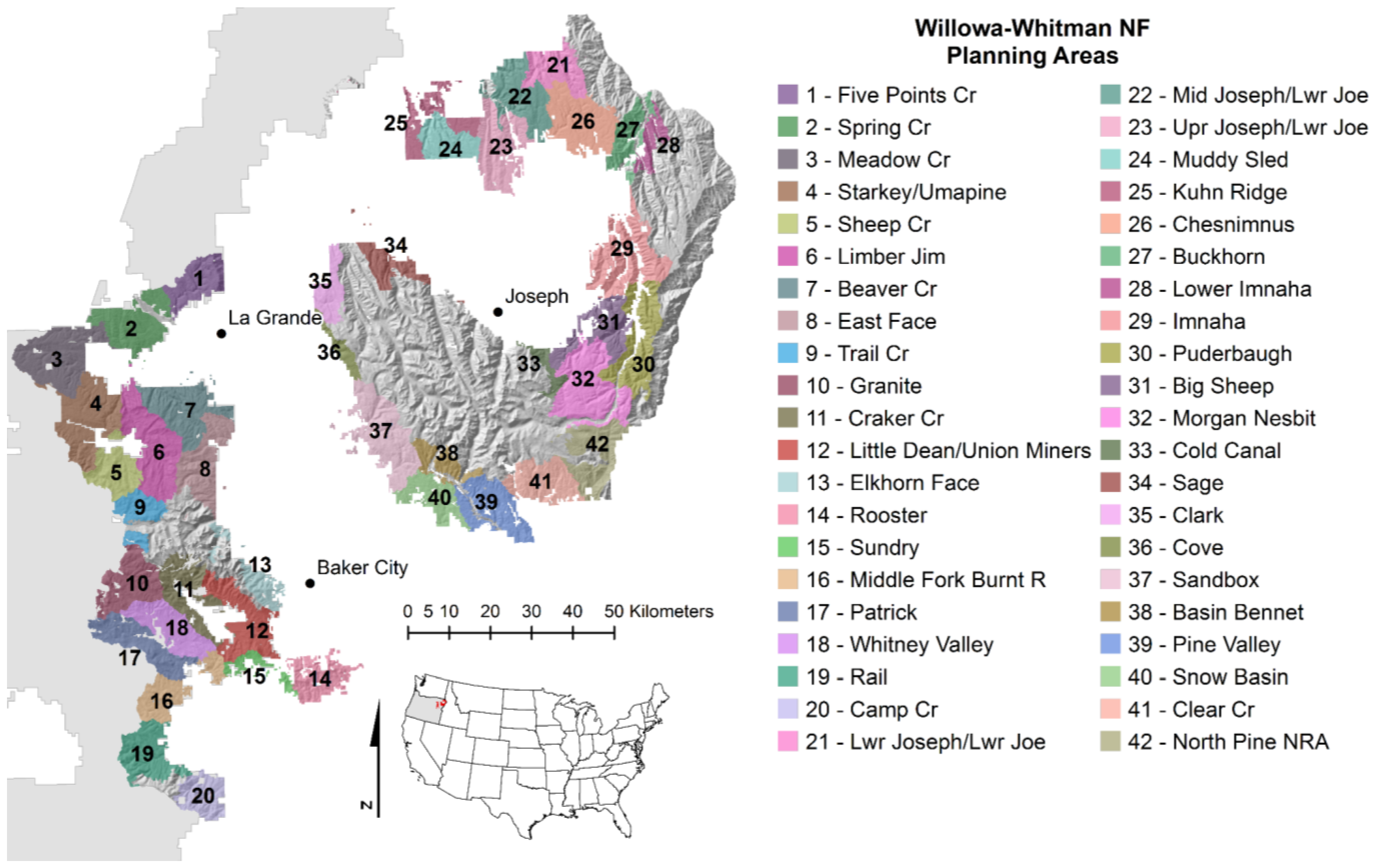
2.1. Study Area

2.2. Modeled Restoration Objectives
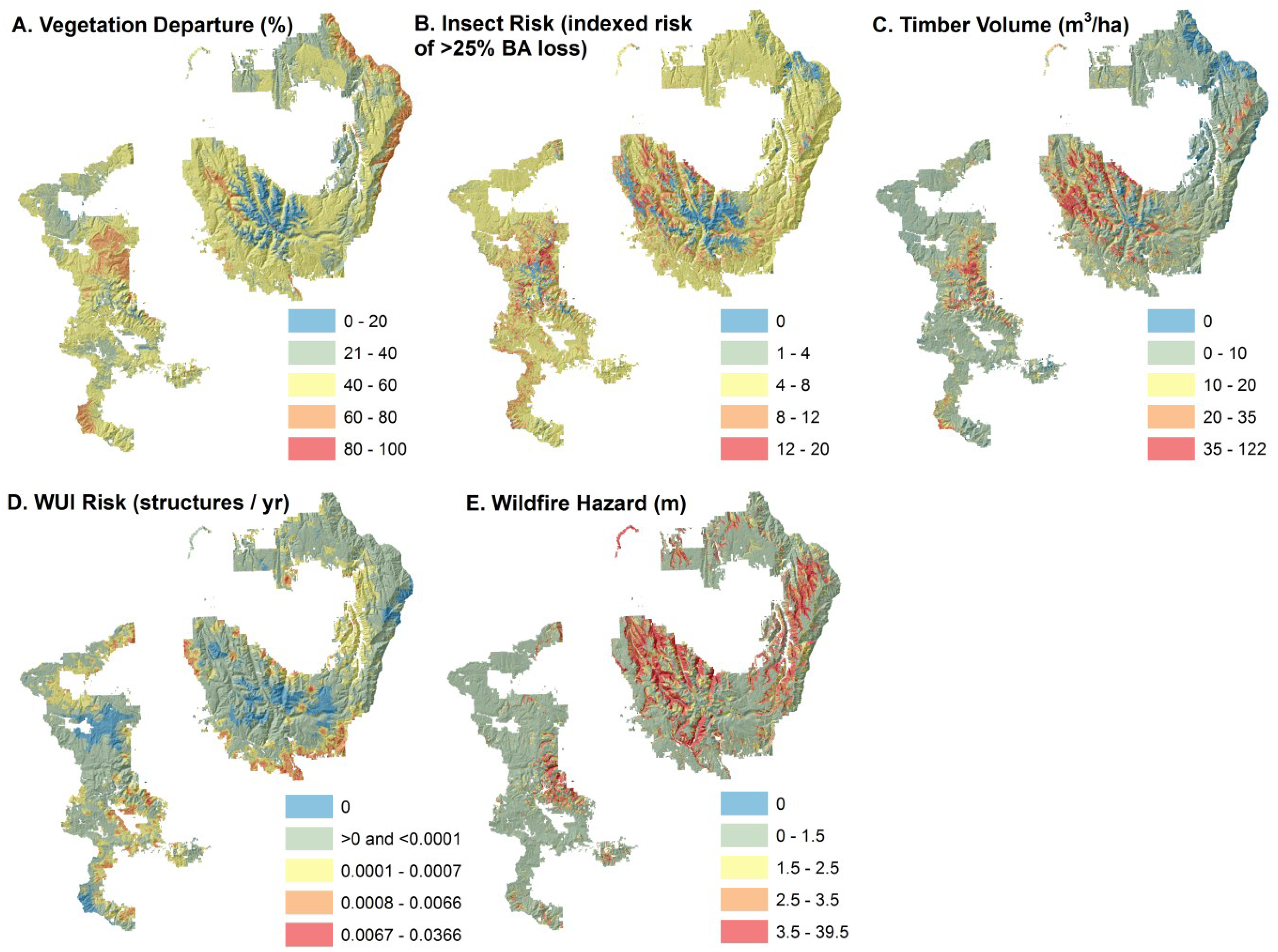
2.3. Vegetation Departure from Reference Conditions

2.4. Insect Risk
2.5. Timber Harvest Volume
2.6. Wildfire Risk to the WUI
2.7. Potential Wildfire Hazard
2.8. Prioritizing Project Areas
2.9. Examining Tradeoffs
3. Results
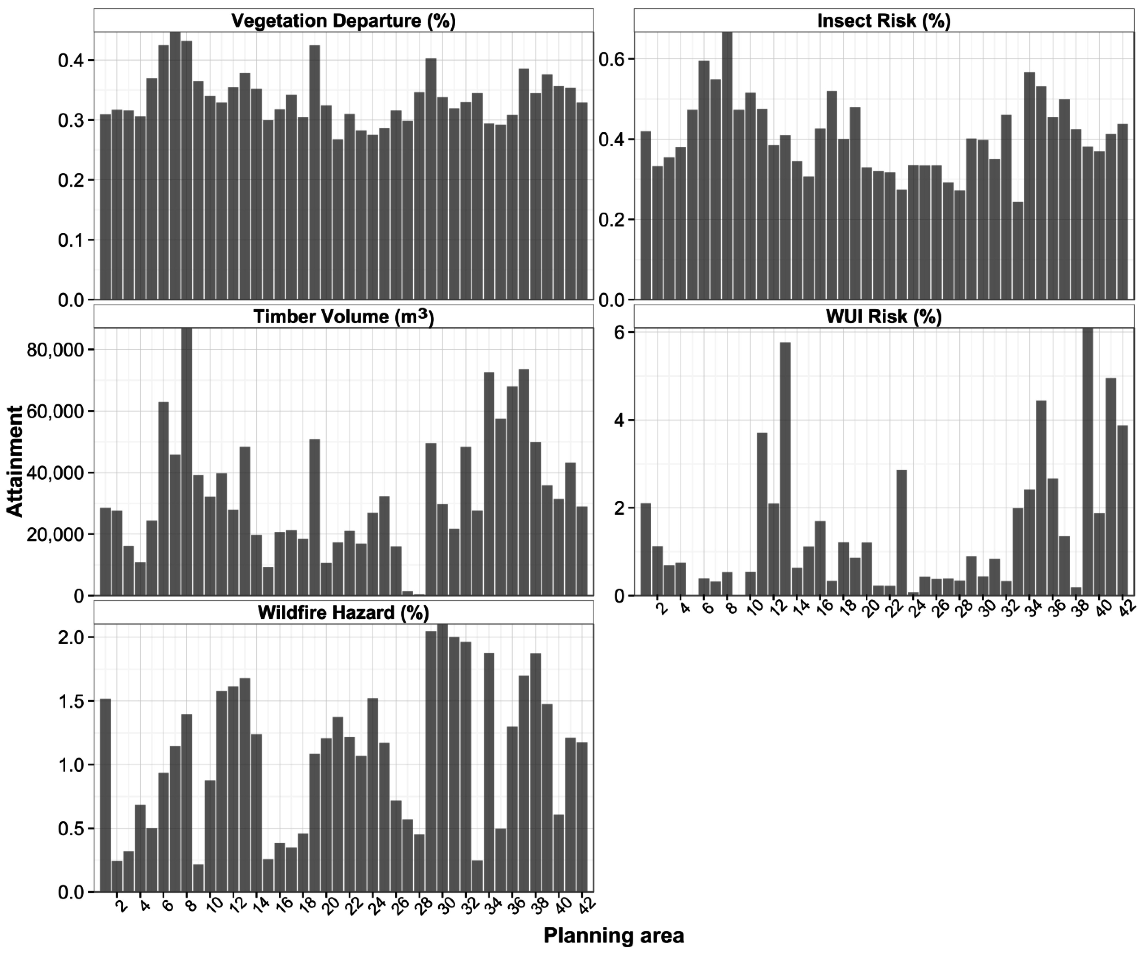
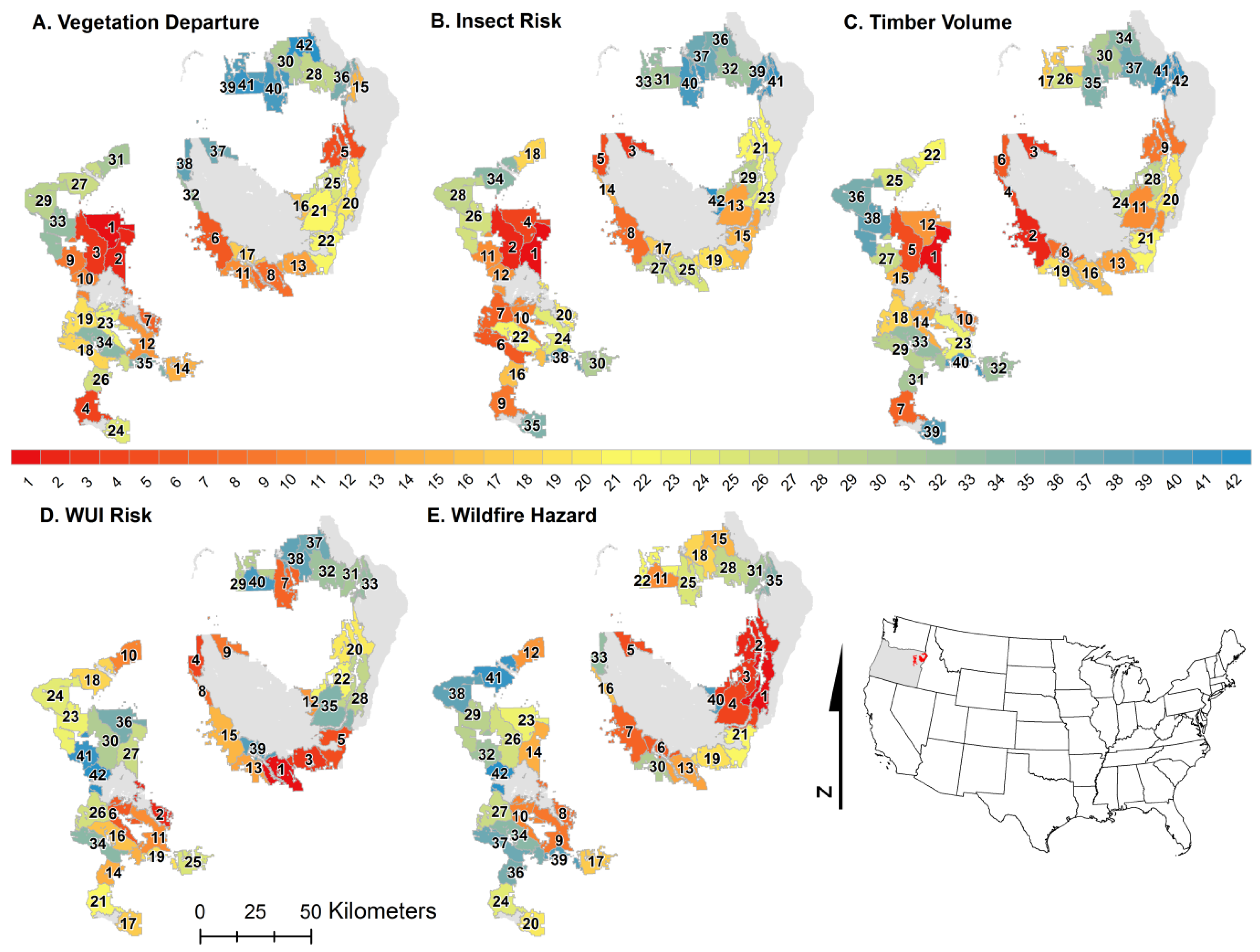
3.1. Priority Planning Areas


| Planning Area | Vegetation Departure | Insect Risk | Timber Volume | WUI Risk | Wildfire Hazard |
|---|---|---|---|---|---|
| Five Points Creek | 31 | 18 | 22 | 10 | 12 |
| Limber Jim | 3 | 2 | 5 | 30 | 26 |
| East Face | 2 | 1 | 1 | 27 | 14 |
| Little Dean/Union Miners | 12 | 24 | 23 | 11 | 9 |
| Rail | 4 | 9 | 7 | 21 | 24 |
| Puderbaugh | 20 | 23 | 20 | 28 | 1 |
| Morgan-Nesbit | 21 | 13 | 11 | 35 | 4 |
| Cold Canal | 16 | 42 | 24 | 12 | 40 |
| Cove | 32 | 14 | 4 | 8 | 16 |
| Sandbox | 6 | 8 | 2 | 15 | 7 |
| Snow Basin | 11 | 27 | 19 | 13 | 30 |
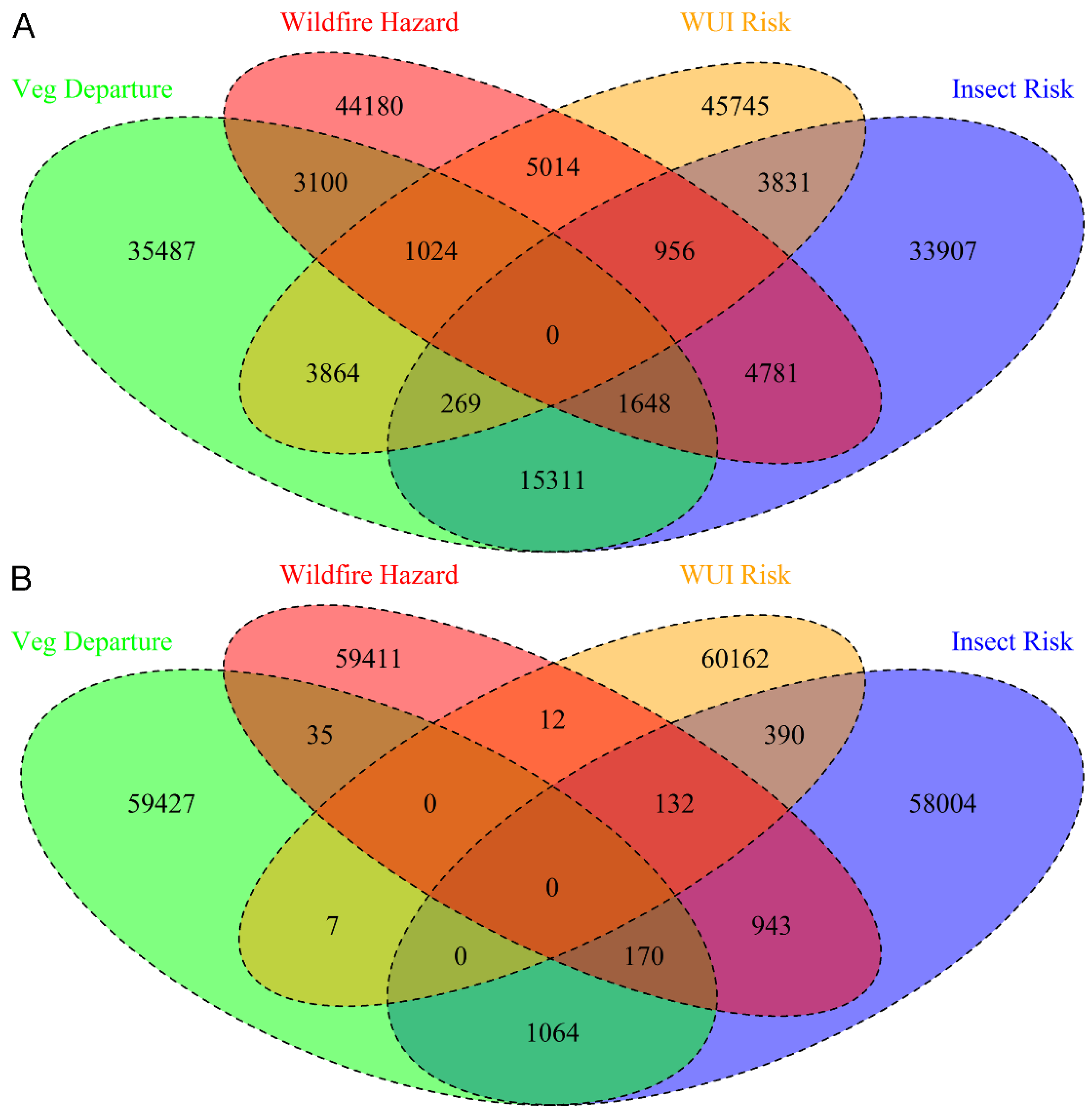
3.2. Restoration Tradeoffs

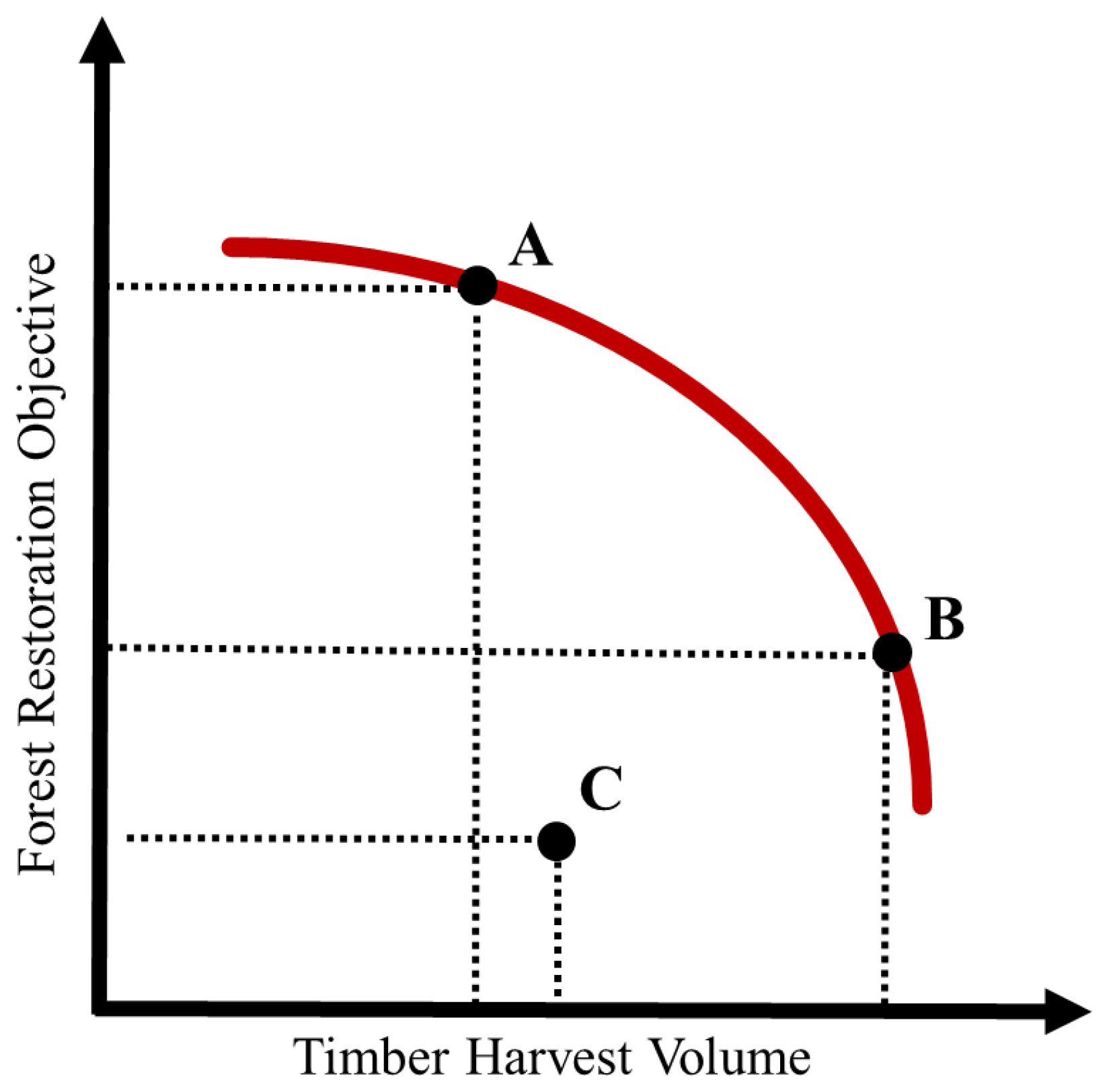
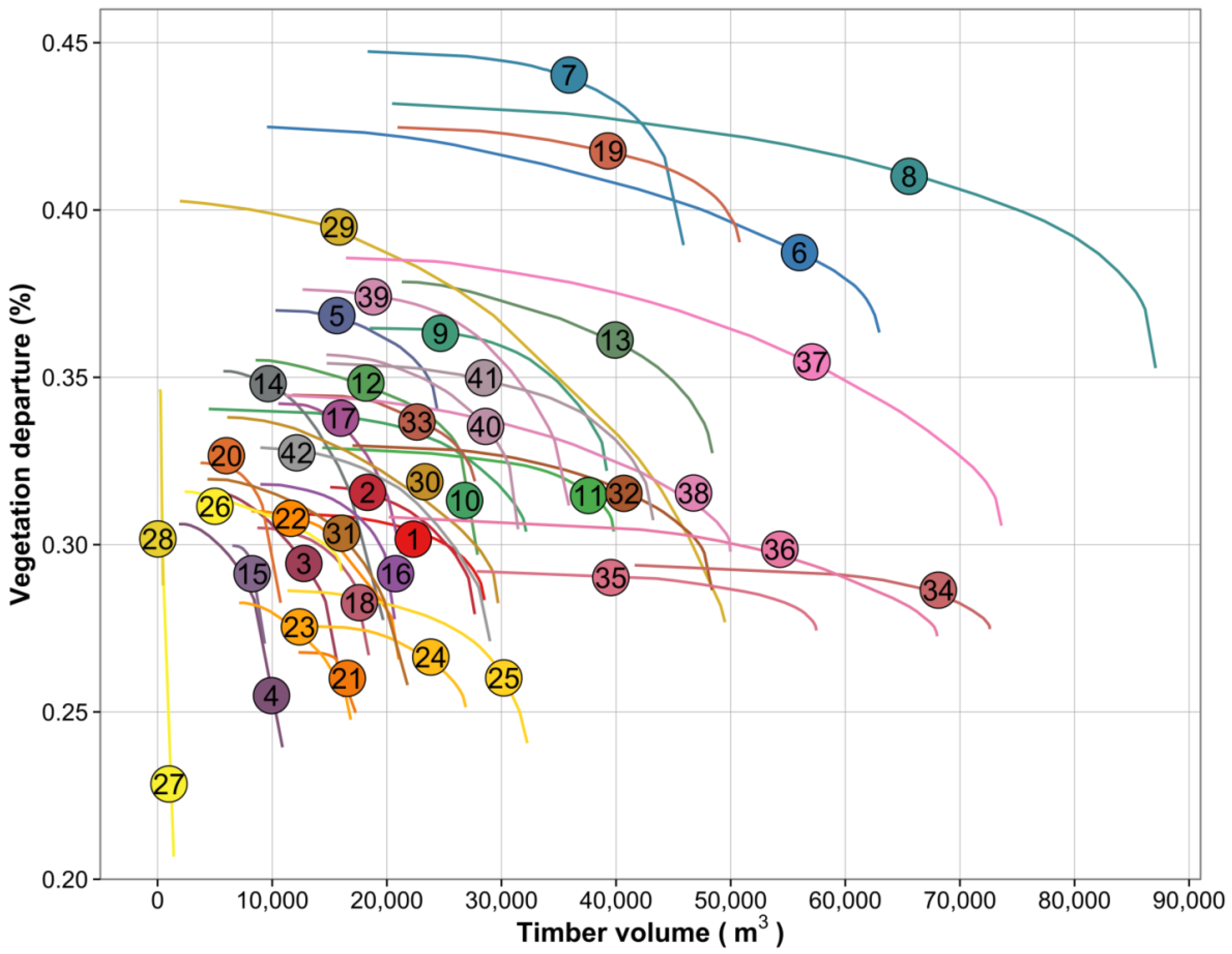
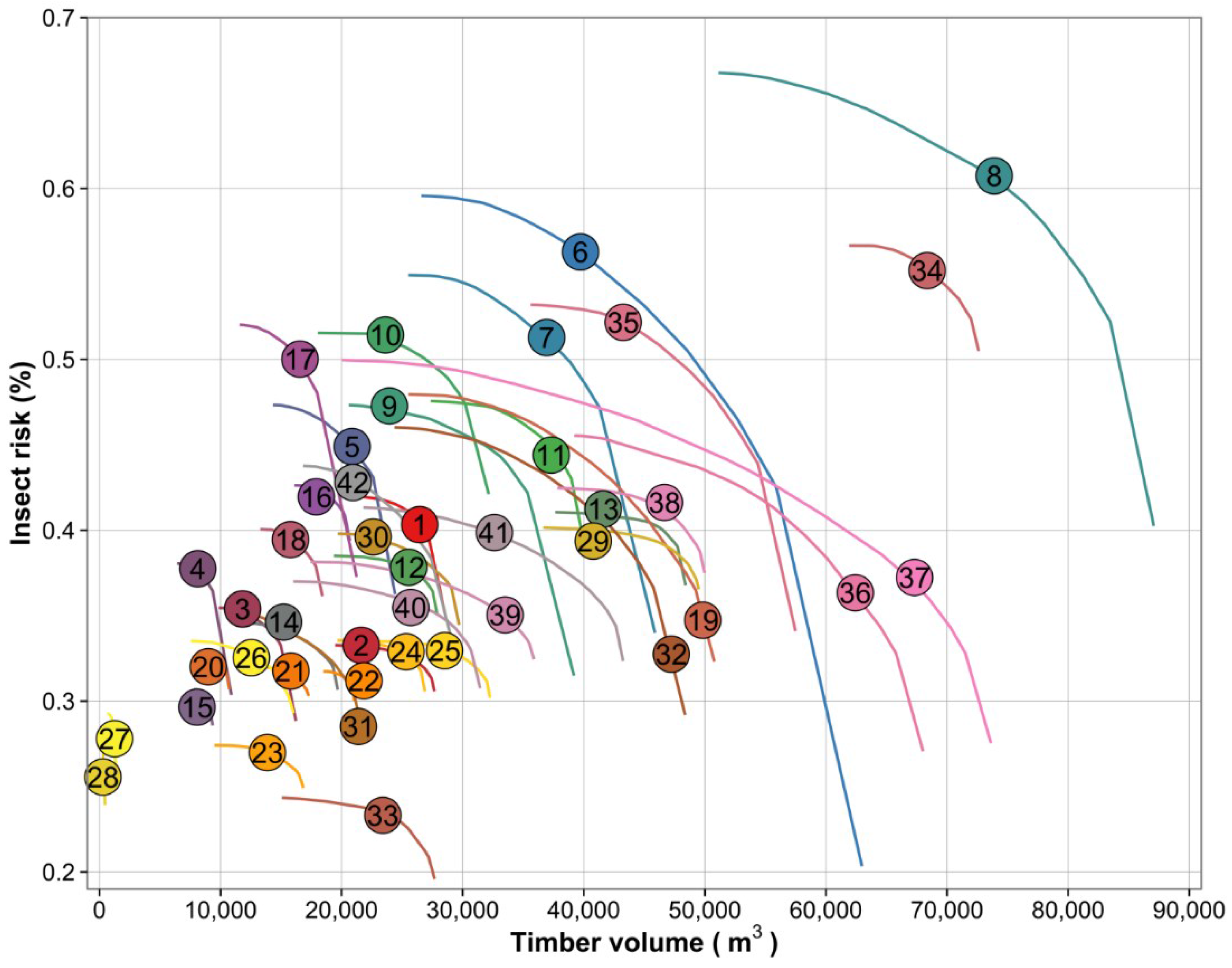
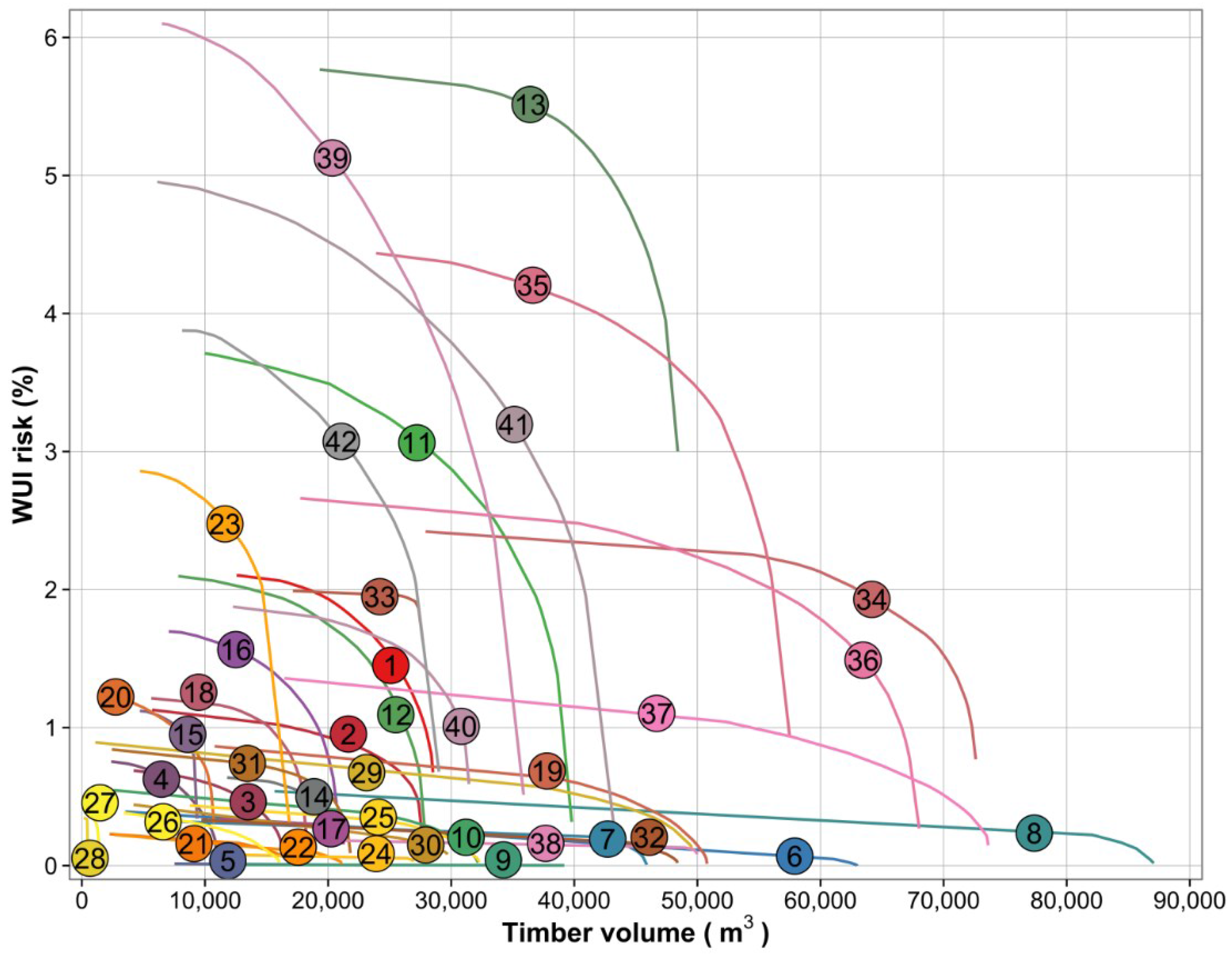
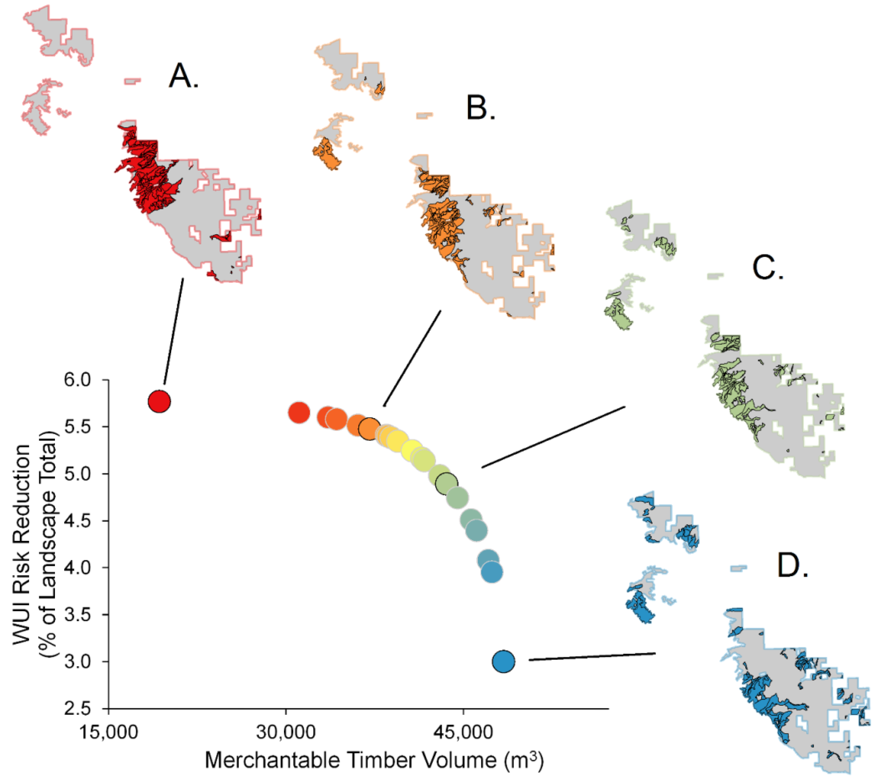
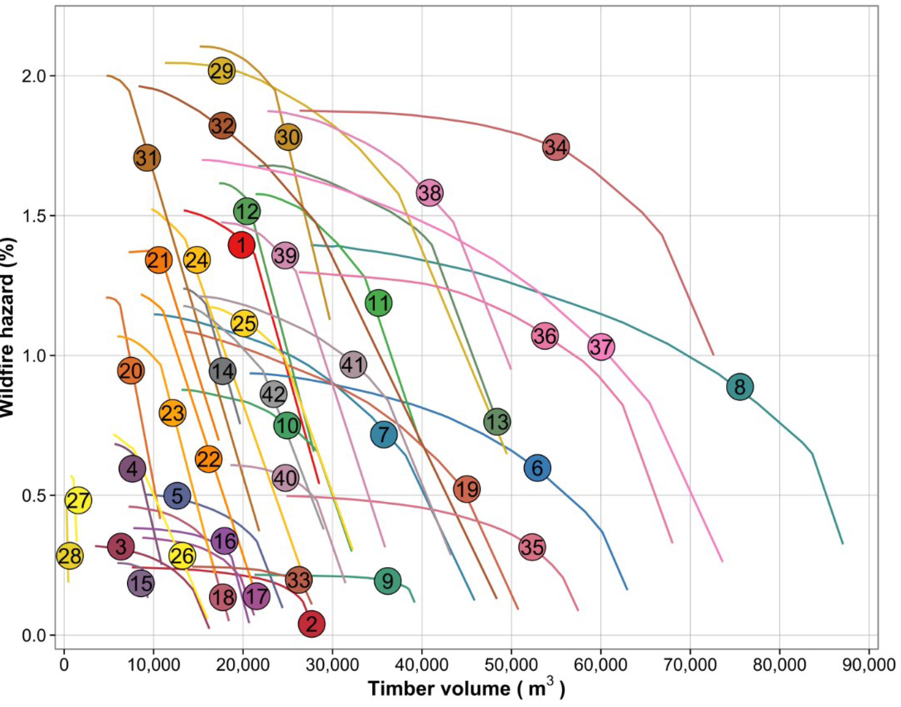
3.3. Production Possibility Frontiers


4. Discussion
Acknowledgments
Author Contributions
Conflicts of Interest
References
- Hessburg, P.F.; Agee, J.K.; Franklin, J.F. Dry forests and wildland fires of the inland Northwest USA: Contrasting the landscape ecology of the pre-settlement and modern eras. For. Ecol. Manag. 2005, 211, 117–139. [Google Scholar] [CrossRef]
- Meddens, A.J.; Hicke, J.A.; Ferguson, C.A. Spatiotemporal patterns of observed bark beetle-caused tree mortality in British Columbia and the western United States. Ecol. Appl. 2012, 22, 1876–1891. [Google Scholar] [CrossRef] [PubMed]
- Aerts, R.; Honnay, O. Forest restoration, biodiversity and ecosystem functioning. BMC Ecol. 2011, 11, 29. [Google Scholar] [CrossRef] [PubMed]
- Westerling, A.L.; Hidalgo, H.G.; Cayan, D.R.; Swetnam, T.W. Warming and earlier spring increase western U.S. forest wildfire activity. Science 2006, 313, 940–943. [Google Scholar] [CrossRef] [PubMed]
- Bentz, B.; Régnière, J.; Fettig, C.; Hansen, E.; Hayes, J.; Hicke, J.; Kelsey, R.; Negrón, J.; Seybold, S. Climate change and bark beetles of the western United States and Canada: Direct and indirect effects. Bioscience 2010, 60, 602–613. [Google Scholar] [CrossRef]
- Hansen, A.J.; Neilson, R.P.; Dale, V.H.; Flather, C.H.; Iverson, L.R.; Currie, D.J.; Shafer, S.; Cook, R.; Bartlein, P.J. Global change in forests: Responses of species, communities, and biomes interactions between climate change and land use are projected to cause large shifts in biodiversity. Bioscience 2001, 51, 765–779. [Google Scholar] [CrossRef]
- USDA Forest Service. Increasing the Pace of Restoration and Job Creation on Our National Forests; United States Department of Agriculture, Forest Service: Washington, DC, USA, 2012; Available online: http://www.fs.fed.us/sites/default/files/media/types/publication/field_pdf/increasing-pace-restoration-job-creation-2012.pdf (accessed on 1 October 2015).
- Food and Agriculture Organization. Global Forest Resources Assessment; Main Report, Report No.: 163; FAO: Rome, Italy, 2010. [Google Scholar]
- Agee, J.K.; Skinner, C.N. Basic principles of forest fuel reduction treatments. For. Ecol. Manag. 2005, 211, 83–96. [Google Scholar] [CrossRef]
- Maron, M.; Cockfield, G. Managing trade-offs in landscape restoration and revegetation projects. Ecol. Appl. 2008, 18, 2041–2049. [Google Scholar] [CrossRef] [PubMed] [Green Version]
- Reynolds, K. EMDS 3.0: A modeling framework for coping with complexity in environmental assessment and planning. Sci. China Ser. E 2006, 49, 63–75. [Google Scholar] [CrossRef]
- Watts, M.E.; Ball, I.R.; Stewart, R.S.; Klein, C.J.; Wilson, K.; Steinback, C.; Lourival, R.; Kircher, L.; Possingham, H.P. Marxan with Zones: Software for optimal conservation based land- and sea-use zoning. Environ. Model. Softw. 2009, 24, 1513–1521. [Google Scholar] [CrossRef]
- Hof, J.; Bevers, M. Spatial Optimization in Ecological Applications; Columbia University Press: New York, NY, USA, 2002; p. 261. [Google Scholar]
- Segura, M.; Ray, D.; Maroto, C. Decision support systems for forest management: A comparative analysis and assessment. Comput. Electron. Agric. 2014, 101, 55–67. [Google Scholar] [CrossRef]
- Rappaport, D.I.; Tambosi, L.R.; Metzger, J.P. A landscape triage approach: Combining spatial and temporal dynamics to prioritize restoration and conservation. J. Appl. Ecol. 2015, 52, 590–601. [Google Scholar] [CrossRef]
- Polasky, S.; Nelson, E.; Camm, J.; Csuti, B.; Fackler, P.; Lonsdorf, E.; Montgomery, C.; White, D.; Arthur, J.; Garber-Yonts, B.; et al. Where to put things? Spatial land management to sustain biodiversity and economic returns. Biol. Conserv. 2008, 141, 1505–1524. [Google Scholar] [CrossRef]
- Levin, N.; Watson, J.E.; Joseph, L.N.; Grantham, H.S.; Hadar, L.; Apel, N.; Perevolotsky, A.; DeMalach, N.; Possingham, H.P.; Kark, S. A framework for systematic conservation planning and management of Mediterranean landscapes. Biol. Conserv. 2013, 158, 371–383. [Google Scholar] [CrossRef]
- Schroter, M.; Rusch, G.M.; Barton, D.N.; Blumentrath, S.; Norden, B. Ecosystem services and opportunity costs shift spatial priorities for conserving forest biodiversity. PLoS ONE 2014, 9, e112557. [Google Scholar] [CrossRef] [PubMed]
- Klein, C.J.; Steinback, C.; Watts, M.; Scholz, A.J.; Possingham, H.P. Spatial marine zoning for fisheries and conservation. Front. Ecol. Environ. 2009, 8, 349–353. [Google Scholar] [CrossRef]
- Klein, C.J.; Tulloch, V.J.; Halpern, B.S.; Selkoe, K.A.; Watts, M.E.; Steinback, C.; Scholz, A.; Possingham, H.P. Tradeoffs in marine reserve design: Habitat condition, representation, and socioeconomic costs. Conserv. Lett. 2013, 6, 324–332. [Google Scholar] [CrossRef]
- Yates, K.L.; Schoeman, D.S.; Klein, C.J. Ocean zoning for conservation, fisheries and marine renewable energy: Assessing trade-offs and co-location opportunities. J. Environ. Manag. 2015, 152, 201–209. [Google Scholar] [CrossRef] [PubMed]
- Kline, J.D.; Mazzotta, M. Evaluating Tradeoffs Among Ecosystem Services in the Management of Public Lands; Report No.: PNW-GTR-865; USDA Forest Service, Pacific Northwest Research Station: Portland, OR, USA, 2012. [Google Scholar]
- Filip, G.M.; Parks, C.A.; Wickman, B.E.; Mitchell, R.G. Tree wound dynamics in thinned and unthinned stands of grand fir, ponderosa pine, and lodgepole pine in eastern Oregon. Northwest Sci. 1995, 69, 276–283. [Google Scholar]
- Wickman, B.E. Forest Health in the Blue Mountains: The Influence of Insects and Diseases; Report No.: PNW-GTR-295; USDA Forest Service, Pacific Northwest Reseach Station: Portland, OR, USA, 1992. [Google Scholar]
- Short, K.C. A spatial database of wildfire in the United States, 1992–2011. Earth Syst. Sci. Data 2014, 6, 1–27. [Google Scholar] [CrossRef]
- Landfire. Landfire Vegetation Departure. 2013. Available online: http://landfire.cr.usgs.gov/viewer/ (accessed on 6 August 2013). [Google Scholar]
- Barrett, S.; Havlina, D.; Jones, J.; Hann, W.; Frame, C.; Hamilton, D.; Schon, K.; DeMeo, T.; Hutter, L.; Menakis, J. Interagency Fire Regime Condition Class (FRCC) Guidebook; Version 3.0. Available online: www.frames.gov/partner-sites/frcc/frcc-guidebook-and-forms/ (accessed on 20 November 2015).
- Rollins, M.; Ward, B.; Dillon, G.; Pratt, S.; Wolf, A. Developing the Landfire Fire Regime Data Products. 2007. Available online: http://www.landfire.gov/downloadfile.php?file=Developing_the_LANDFIRE_Fire_Regime_Data_Products.pdf (accessed on 15 May 2015). [Google Scholar]
- Jennings, M.; (Wallowa-Whitman National Forest, La Grande Ranger District, La Grande, OR, USA). Insect risk data for the Wallowa-Whitman National Forest. Personal communication, 2014. [Google Scholar]
- Ohmann, J.L.; Gregory, M.J. Predictive mapping of forest composition and structure with direct gradient analysis and nearest-neighbor imputation in coastal Oregon, USA. Can. J. For. Res. 2002, 32, 725–741. [Google Scholar] [CrossRef]
- Dixon, G.E. Essential FVS: A User’s Guide to the Forest Vegetation Simulator; USDA Forest Service, Forest Management Service Center: Fort Collins, CO, USA, 2002; Available online: http://www.fs.fed.us/fmsc/ftp/fvs/docs/gtr/EssentialFVS.pdf (accessed on 1 October 2015).
- Ager, A.A.; McMahan, A.J.; Barrett, J.J.; McHugh, C.W. A simulation study of thinning and fuel treatments on a wildland-urban interface in eastern Oregon, USA. Landsc. Urban Plan. 2007, 80, 292–300. [Google Scholar] [CrossRef]
- Ager, A.A.; Vaillant, N.M.; Finney, M.A. A comparison of landscape fuel treatment strategies to mitigate wildland fire risk in the urban interface and preserve old forest structure. For. Ecol. Manag. 2010, 259, 1556–1570. [Google Scholar] [CrossRef]
- Reineke, L.H. Perfecting a stand-density index for even-aged forests. J. Agric. Res. 1933, 46, 627–638. [Google Scholar]
- Cochran, P.H.; Geist, J.M.; Clemens, D.L.; Clausnitzer, R.R.; Powell, D.C. Suggested Stocking Levels for Forest Stands in Northeastern Oregon and Southeastern Washington; Report No.: PNW-RN-513; USDA Forest Service, Pacific Northwest Research Station: Portland, OR, USA, 1994. [Google Scholar]
- Hall, E.C. Pacific Northwest Ecoclass Codes for Seral and Potential Natural Communities; Report No.: PNW-GTR-418; USDA Forest Service, Pacific Northwest Research Station: Portland, OR, USA, 1998. [Google Scholar]
- Johnson, C.G., Jr.; Clausnitzer, R.R. Plant Associations of the Blue and Ochoco Mountains; Report No.: R6-ERW-TP-036-92; USDA Forest Service, Pacific Northwest Region: Portland, OR, USA, 1992. [Google Scholar]
- Keyser, C.E.; Dixon, G.E. Blue Mountains (BM) Variant Overview—Forest Vegetation Simulator; USDA Forest Service, Forest Management Service Center: Fort Collins, CO, USA, 2015. [Google Scholar]
- Radeloff, V.C.; Hammer, R.B.; Stewart, S.I.; Fried, J.S.; Holcomb, S.S.; McKeefry, J.F. The wildland-urban interface in the United States. Ecol. Appl. 2005, 15, 799–805. [Google Scholar] [CrossRef]
- Ager, A.A.; Day, M.A.; McHugh, C.W.; Short, K.; Gilbertson-Day, J.; Finney, M.A.; Calkin, D.E. Wildfire exposure and fuel management on western US national forests. J. Environ. Manag. 2014, 145, 54–70. [Google Scholar] [CrossRef] [PubMed]
- Finney, M.A.; McHugh, C.W.; Grenfell, I.C.; Riley, K.L.; Short, K.C. A simulation of probabilistic wildfire risk components for the continental United States. Stoch. Environ. Res. Risk Assess. 2011, 25, 973–1000. [Google Scholar] [CrossRef]
- Western Regional Climate Center. RAWS USA Climate Archive. 2014. Available online: http://www.raws.dri.edu/ (accessed on 1 October 2015).
- Forests and Rangelands. Fire Program Analysis. 2010. Available online: http://www.fpa.nifc.gov/ (accessed on 28 November 2012). [Google Scholar]
- Finney, M.A. An overview of FlamMap fire modeling capabilities. In Proceedings of the Fuels Management—How to Measure Success, RMRS-P-41, Portland, OR, USA, 28–30 March 2006; Andrews, P.L., Butler, B.W., Eds.; USDA Forest Service, Rocky Mountain Research Station: Fort Collins, CO, USA, 2006; pp. 213–220. [Google Scholar]
- Rollins, M.G. Landfire: A nationally consistent vegetation, wildland fire, and fuel assessment. Int. J. Wildland Fire 2009, 18, 235–249. [Google Scholar] [CrossRef]
- Landfire. Homepage of the Landfire Project. 2013. Available online: http://www.landfire.gov/index.php (accessed on 26 August 2009). [Google Scholar]
- Scott, J.H.; Burgan, R.E. Standard Fire Behavior Fuel Models: A Comprehensive Set for Use with Rothermel’s Surface Fire Spread Model; Report No.: RMRS-GTR-153; USDA Forest Service, Rocky Mountain Research Station: Fort Collins, CO, USA, 2005; Available online: http://treesearch.fs.fed.us/pubs/9521 (accessed on 20 November 2015).
- Ager, A.A.; Vaillant, N.M.; McMahan, A. Restoration of fire in managed forests: A model to prioritize landscapes and analyze tradeoffs. Ecosphere 2013, 4, 29. [Google Scholar] [CrossRef]
- Brown, R.T.; Agee, J.K.; Franklin, J.F. Forest restoration and fire: Principles in the context of place. Conserv. Biol. 2004, 18, 903–912. [Google Scholar] [CrossRef]
- USDA Forest Service. Ecosystem Restoration: A Framework for Restoring and Maintaining the National Forests and Grasslands; USDA Forest Service: Washington, DC, USA, 2006; Available online: http://www.fs.fed.us/restoration/documents/RestFramework_final_010606.pdf (accessed on 20 August 2015).
- Johnson, J.F.; Bengston, D.N.; Fan, D.P.; Nelson, K.C. US policy response to the fuels management problem: An analysis of the public debate about the Healthy Forests Initiative and the Healthy Forests Restoration Act. In Proceedings of the Fuels Management—How to Measure Success, RMRS-P-41, Portland, OR, USA, 28–30 March 2006; Andrews, P.L., Butler, B.W., Eds.; USDA Forest Service, Rocky Mountain Research Station: Fort Collins, CO, USA, 2006; pp. 59–66. [Google Scholar]
- Lachapelle, P.R.; McCool, S.F. The role of trust in community wildland fire protection planning. Soc. Nat. Resour. 2012, 25, 321–335. [Google Scholar] [CrossRef]
- Butler, W.H.; Goldstein, B.E. The US Fire Learning Network: Springing a rigidity trap through multiscalar collaborative networks. Ecol. Soc. 2010, 15, 21. [Google Scholar]
- Iverson, D.C.; Alston, R.M. The Genesis of Forplan: A Historical and Analytical Review of Forest Service Planning Models; Report No.: INT-214; USDA Forest Service, Intermountain Research Station: Ogden, UT, USA, 1986. [Google Scholar]
- Mowrer, H.T. Decision Support Systems for Ecosystem Management: An Evaluation of Existing Systems; Report No.: RM-GTR-296; USDA Forest Service, Rocky Mountain Forest and Range Experiment Station: Fort Collins, CO, USA, 1997. [Google Scholar]
- Hemstrom, M.A.; Merzenich, J.; Reger, A.; Wales, B. Integrated analysis of landscape management scenarios using state and transition models in the upper Grande Ronde River Subbasin, Oregon, USA. Landsc. Urban Plan. 2007, 80, 198–211. [Google Scholar] [CrossRef]
- USDA. 36 CFR Part 219. National forest system land management planning. Fed. Regist. 2012, 77, 21162–21276. [Google Scholar]
- Reynolds, K.M. EMDS: Using a logic framework to assess forest ecosystem sustainability. J. For. 2001, 99, 26–30. [Google Scholar]
- Allan, J.D.; McIntyre, P.B.; Smith, S.D.P.; Halpern, B.S.; Boyer, G.L.; Buchsbaum, A.; Burton, G.A., Jr.; Campbell, L.M.; Chadderton, W.L.; Ciborowski, J.J.H.; et al. Joint analysis of stressors and ecosystem services to enhance restoration effectiveness. Proc. Natl. Acad. Sci. USA 2013, 110, 372–377. [Google Scholar] [CrossRef] [PubMed]
- Groeneveld, R.; Grashof-Bokdam, C.; van Ierland, E. Metapopulations in agricultural landscapes: A spatially explicit trade-off analysis. J. Environ. Plan. Manag. 2005, 48, 527–547. [Google Scholar] [CrossRef]
© 2015 by the authors; licensee MDPI, Basel, Switzerland. This article is an open access article distributed under the terms and conditions of the Creative Commons by Attribution (CC-BY) license (http://creativecommons.org/licenses/by/4.0/).
Share and Cite
Vogler, K.C.; Ager, A.A.; Day, M.A.; Jennings, M.; Bailey, J.D. Prioritization of Forest Restoration Projects: Tradeoffs between Wildfire Protection, Ecological Restoration and Economic Objectives. Forests 2015, 6, 4403-4420. https://doi.org/10.3390/f6124375
Vogler KC, Ager AA, Day MA, Jennings M, Bailey JD. Prioritization of Forest Restoration Projects: Tradeoffs between Wildfire Protection, Ecological Restoration and Economic Objectives. Forests. 2015; 6(12):4403-4420. https://doi.org/10.3390/f6124375
Chicago/Turabian StyleVogler, Kevin C., Alan A. Ager, Michelle A. Day, Michael Jennings, and John D. Bailey. 2015. "Prioritization of Forest Restoration Projects: Tradeoffs between Wildfire Protection, Ecological Restoration and Economic Objectives" Forests 6, no. 12: 4403-4420. https://doi.org/10.3390/f6124375