Article

Windthrow Detection in European Forests with Very High-Resolution Optical Data

1
Institute of Surveying, Remote Sensing and Land Information (IVFL), University of Natural Resources and Life Sciences, Vienna (BOKU), Peter-Jordan-Strasse 82, 1190 Vienna, Austria
2
Bavarian State Institute of Forestry (LWF), Department of Information Technology, Hans-Carl-von-Carlowitz-Platz 1, 85354 Freising, Germany
3
German Aerospace Center (DLR), German Remote Sensing Data Center, Land Surface, 82234 Wessling, Germany
*
Author to whom correspondence should be addressed.
Forests 2017, 8(1), 21; https://doi.org/10.3390/f8010021
Submission received: 14 October 2016 / Revised: 16 December 2016 / Accepted: 31 December 2016 / Published: 6 January 2017
(This article belongs to the Special Issue Remote Sensing of Forest Disturbance)

Abstract

:
With climate change, extreme storms are expected to occur more frequently. These storms can cause severe forest damage, provoking direct and indirect economic losses for forestry. To minimize economic losses, the windthrow areas need to be detected fast to prevent subsequent biotic damage, for example, related to beetle infestations. Remote sensing is an efficient tool with high potential to cost-efficiently map large storm affected regions. Storm Niklas hit South Germany in March 2015 and caused widespread forest cover loss. We present a two-step change detection approach applying commercial very high-resolution optical Earth Observation data to spot forest damage. First, an object-based bi-temporal change analysis is carried out to identify windthrow areas larger than 0.5 ha. For this purpose, a supervised Random Forest classifier is used, including a semi-automatic feature selection procedure; for image segmentation, the large-scale mean shift algorithm was chosen. Input features include spectral characteristics, texture, vegetation indices, layer combinations and spectral transformations. A hybrid-change detection approach at pixel-level subsequently identifies small groups of fallen trees, combining the most important features of the previous processing step with Spectral Angle Mapper and Multivariate Alteration Detection. The methodology was evaluated on two test sites in Bavaria with RapidEye data at 5 m pixel resolution. The results regarding windthrow areas larger than 0.5 ha were validated with reference data from field visits and acquired through orthophoto interpretation. For the two test sites, the novel object-based change detection approach identified over 90% of the windthrow areas (≥0.5 ha). The red edge channel was the most important for windthrow identification. Accuracy levels of the change detection at tree level could not be calculated, as it was not possible to collect field data for single trees, nor was it possible to perform an orthophoto validation. Nevertheless, the plausibility and applicability of the pixel-based approach is demonstrated on a second test site.

1. Introduction

In the last few decades, Europe was hit by a series of heavy storms, such as Vivian and Wiebke in 1990, Lothar in 1999, followed by Kyrill in 2007. In March 2015, storm Niklas caused widespread forest damage in South Germany. It is expected that in the future the frequency of severe storms will further increase in Europe [1,2]. These storms damaged areas were often correlated with subsequent insect outbreaks, mainly European spruce bark beetle Ips typographus (L.). In Europe, abiotic wind disturbances and biotic bark beetle infestations are the main factors for causing forest disturbances [2]. Between 1950 and 2000 the approximate average annual storm damage in Europe was 18.7 million m3 of wood, with most of the storm damage occurring in Central Europa and the Alps [1]. In the same period, the average annual wood volume damage by bark beetles was 2.9 million m3 per year [1]. Thus, the affected forest areas need to be localized quickly to assess the damage and to minimize the impact of biotic subsequent damage, as storm damaged trees are providing breeding materials for the insects [1,3].
Efficient and cost-effective tools for a fast and reliable detection of the vast windthrow areas are still missing. Previous studies have shown the general suitability of passive optical Earth Observation (EO) sensors for forest disturbances detection [4,5,6,7,8,9,10,11].
These studies mainly apply pixel-based approaches to medium-resolution (MR) data (Table 1). Compared to MR data, high (HR) to very high resolution (VHR) images display much more detail of the Earth’s surface, thus enabling the detection of fine-scale tree damage, which MR data is either unable or limited in its ability to detect. Despite these characteristics, VHR images are less often applied for evaluating forest cover change [12], probably related to the high costs involved with data acquisition and data storing for large areas. Only a few recent studies [7,10,13,14] use HR to VHR satellite imagery for forest disturbance monitoring. As more and more VHR satellites are launched into orbit, and costs for VHR data are continuously decreasing, this data can be a sufficient data source to detect mainly small scale disturbances in forests.
Several change detection (CD) methods exist identifying changes in satellite images, which also can be used for the assessment of abrupt forest cover loss. The recent studies of Chen et al. [22], Hussain et al. [23], Hecheltjen et al. [24], Bovolo and Bruzzone [25], and Tewkesbury et al. [26] give a broad overview of established CD techniques. For a synopsis of forest disturbance CD studies, the reader is referred to Chehata et al. [12].
Generally, CD techniques can be differentiated in pixel-based analysis (PBA) and object-based image analysis (OBIA) [15,17,26]. In OBIA, instead of analyzing single pixels, typically image segmentation is applied first. OBIA is particularly useful when carrying out a CD with VHR imagery, since VHR pixels are in the size of 1 m (measurement unit) and therefore are often smaller than the land surface object (i.e., tree or group of trees) that needs to be detected (mapping unit). Thus, the object size can be scaled to the size of the studied feature [27]. A further advantage of OBIA is that per image-object, statistical, and geometrical measures can be computed in addition to spectral information, which can increase change detection accuracy [22,28].
In this paper, we aim to demonstrate that passive VHR EO satellites provide detailed information about the size and location of the storm loss areas. Large damaged areas are usually easily detected and cleared, smaller areas often not. The remaining dead trees can be very problematic for further bark beetle infestation. Thus, in our study we specially focus on detecting small-scale damages to provide fast information for foresters.
Therefore, the images are taken in a narrow period before and after the storm. As such, mainly forest changes caused by the storm are detectable, which is the focus of our interest. Further, we wanted to capture by applying Random Forest feature selection the spectral characteristics, texture, vegetation indices, and layer combinations that are most suitable for detecting changes caused by windthrow.
Furthermore, we wanted to explore the potential of the red edge spectral region for windthrow detection. In our study, we applied VHR RapidEye data comprising a red edge channel that was centered at 710 nm. Recent studies have shown the performance of red edge bands in facilitating important information on the state of vegetation and their benefit for vegetation monitoring [29,30,31]. In 2015, Sentinel-2A satellite has been launched. The data is globally and freely available, and within the next couple of months, two identical satellites (Sentinel-2A and 2B) will be in orbit, acquiring imagery of land’s spectral properties in up to 10 m spatial resolution every five days, thereby providing dense time series. Sentinel-2 multispectral imager is the first HR sensor to include three red edge bands. RapidEye’s red edge band is close to Sentinel-2’s band 5 [32], hence our findings can support future windthrow analysis with Sentinel-2 data.
As storms such as Niklas often cause different kinds of damage patterns, ranging from scattered tree damage to compact, homogeneous areas with up to several hectares, we aimed for the identification of two sizes of damaged forest areas:
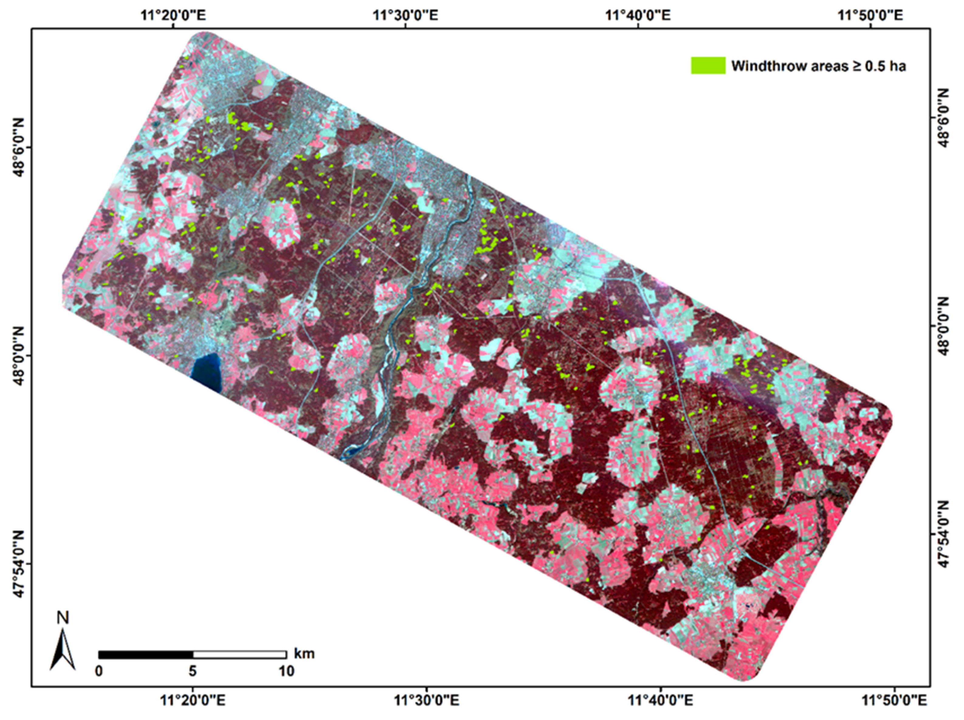
  • windthrow areas ≥0.5 ha, and
  • groups consisting of only few fallen trees (both tree fall-gaps and freestanding groups).

2. Materials and Methods

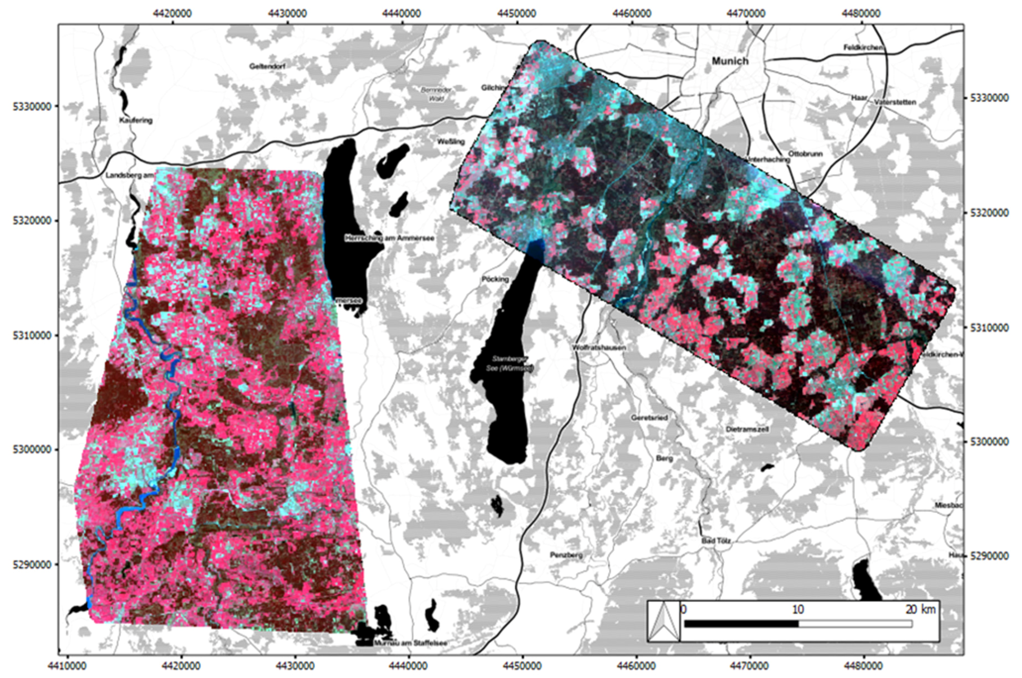
2.1. Storm Niklas and Study Area

Storm Niklas hit Bavaria, Germany, on 31 March 2015 and caused severe damage. Niklas reached peak gusts up to 192 km/h in the Bavarian Alps and up to 120 km/h in the lowlands, and was one of the strongest spring storms in the last 30 years [33]. The core area affected by the storm was the region between the south of Munich and the Alps.
Niklas caused a heterogeneous damage pattern: mainly small groups and single fallen trees, as well as large-scale storm loss in a temperate forest. We performed our study on two test sites in Bavaria, Germany (see Figure 1), which presented both of the two damage patterns. The first site was selected for method development, while the second site was used for method validation.
The first study area Munich South is situated south of the city of Munich (48°0′ N, 11°32′ E, 530 to 750 m above sea level (a.s.l.)), covering an area of approximately 720 km2. The zone is located within the Munich gravel plain and is characterized by very low terrain variation. Approximately 53% of the site is covered by temperate forest, with Norway spruce (Picea abies (L.) Karst) being the dominant tree species (Bavarian State Institute of Forestry: pers. communication). The forests have been hit by the European windstorms Vivian and Wiebke in 1990; since then, forest owners pushed for a conversion into hardwood rich mixed forests [34].
The second study site Landsberg (840 km2) is located west of Munich, near the city of Landsberg (47°53′ N, 10°58′ E, 550–820 m a.s.l.). The region is characterized as alpine foothills with a hilly morainic topography. Approximately one third of the area is covered by forests. Norway spruce forests, pure as well as mixed with European beech (Fagus sylvatica L.) are the main forest types (Bavarian State Institute of Forestry: pers. communication).

2.2. RapidEye Data Set

For the windthrow detection, RapidEye scenes before and after the storm were acquired. RapidEye offers five spectral bands at 5 m spatial resolution: blue (B), green (G), red (R), red edge (RE), and near infrared (NIR). Data are delivered in tiles of 25 × 25 km2. As five identical satellites are in orbit, in principle a daily revisiting can be achieved (ignoring cloud cover). When satellites need to be pointed, however, substantial off-nadir views can occur.
For both test sites, the pre-storm images were acquired on 18 March 2015, 13 days before the storm. The post-storm image of Munich South was taken on 10 April 2015, 10 days after the storm. The post-storm image of Landsberg was acquired on 19 April 2015, 19 days after the storm. All images are nearly cloud free, but with some haze. The pre-storm images also have some snow patches. Vegetation changes in the image are expected to be mainly caused by the storm event, due to the short period between the acquisitions dates (23 days for Munich South and 32 days for Landsberg). Table 2 summarizes the main characteristics of the acquired RapidEye data.
Before mosaicking the single tiles (25 × 25 km2), radiance was transformed into top of atmosphere (TOA) reflectance following BlackBridge [35]. A normalization for differences in sun zenith angles in the TOA correction is expected to be sufficient for the detection of abrupt vegetation changes [36]. No information about aerosol loads and water vapor contents were available to run a proper atmospheric correction.
Correctly co-registered images are crucial for change detection analysis. Therefore, all scenes were acquired as orthorectified (level 3A) products. No further georectification was necessary, since the images were overlaying accurately with orthophotos.

2.3. Reference Data

Field surveys were conducted by Bavarian State Institute of Forestry in the study regions in April 2015, a few days after the storm. Several damaged areas were thereby mapped using Garmin GPSMAP 64 devices. In addition, information was collected about windthrow size and type (e.g., single fallen tree, stand, or large-scale windfall), tree damage (e.g., broken branches, tree split, uprooted trees), and the main affected tree species. Table 3 summarize the main characteristics of these field surveys, which were used for a first validation of the developed method.
In addition, and for large-scale validation, another reference data set was created from orthophotos (see Table 4). For this purpose, false-color infrared orthophotos with 20 cm spatial resolution were used, which were acquired in June and July 2015. The orthophotos were visually interpreted and windfalls (≥0.5 ha) were manually digitized. The delineated windthrow areas were cross-checked with older pre-storm orthophotos and RapidEye scenes.
It should be noted that the reference obtained from the orthophoto is potentially biased. The orthophotos were acquired three (Munich South) to four months (Landsberg) after storm Niklas. During this time, some windfall areas had been cleared and adjacent (not damaged) trees were removed for forest protection reasons (Bavarian State Institute of Forestry: pers. communication). Thus, some cleared areas are larger in size than the windthrow damaged areas.

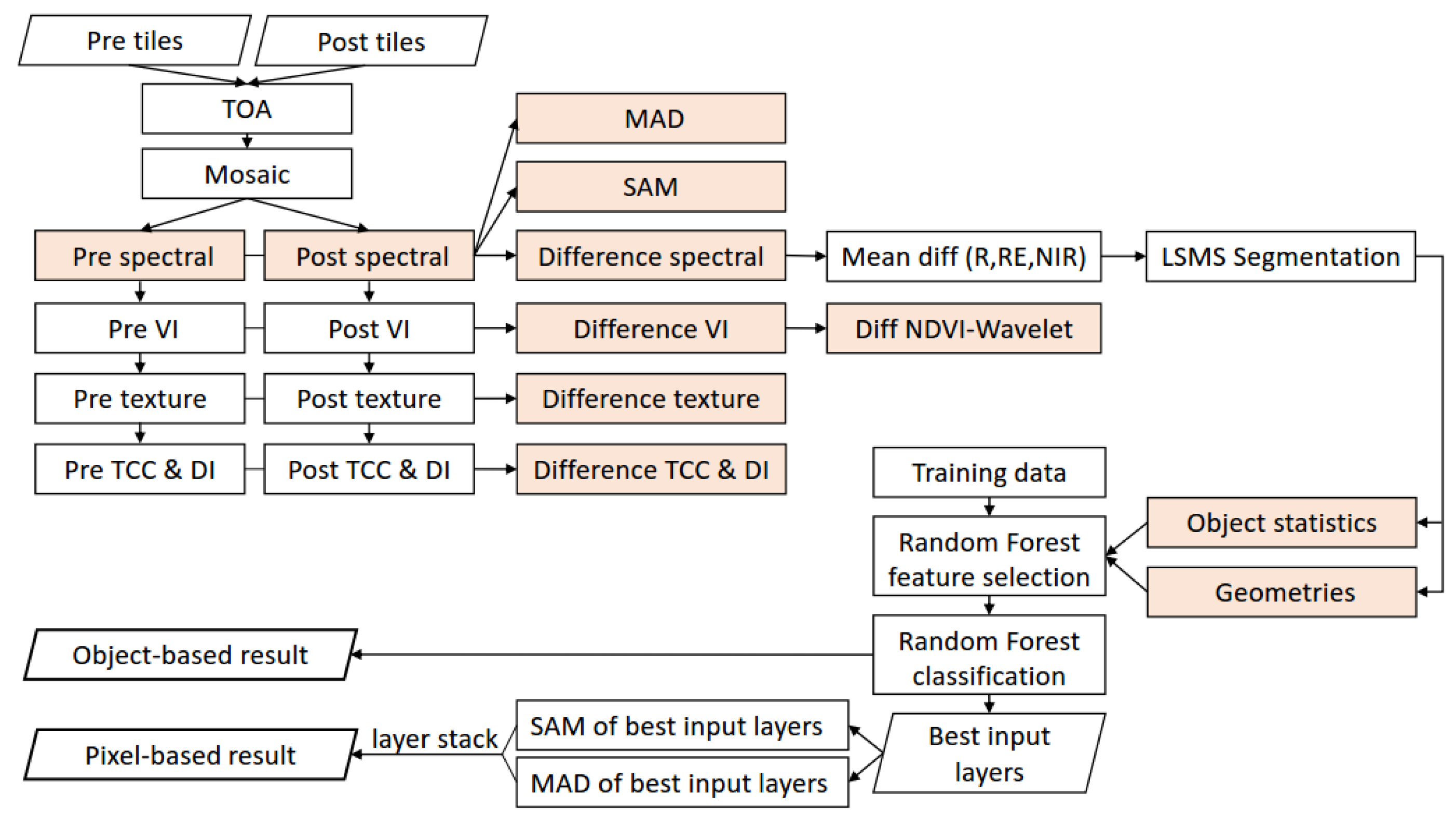
2.4. Method/Approach

To map and identify windthrow areas, a two-step approach was applied. First, a bi-temporal object-based change detection was performed, applying a feature selection and classification with Random Forest (RF). Image segmentation was carried out with large-scale mean shift (LSMS) algorithm. In a second step, smaller windthrow areas were detected at pixel-level using a hybrid technique. The overall approach is outlined in Figure 2; the four main parts of the approach, described in Section 2.4.1, Section 2.4.2, Section 2.5.1, Section 2.5.2, Section 2.5.3, Section 2.5.4 and Section 2.6 were:
  • calculation of input layers,
  • image segmentation,
  • RF feature selection and object-based change classification, and
  • development of pixel-based approach

2.4.1. Input Variables
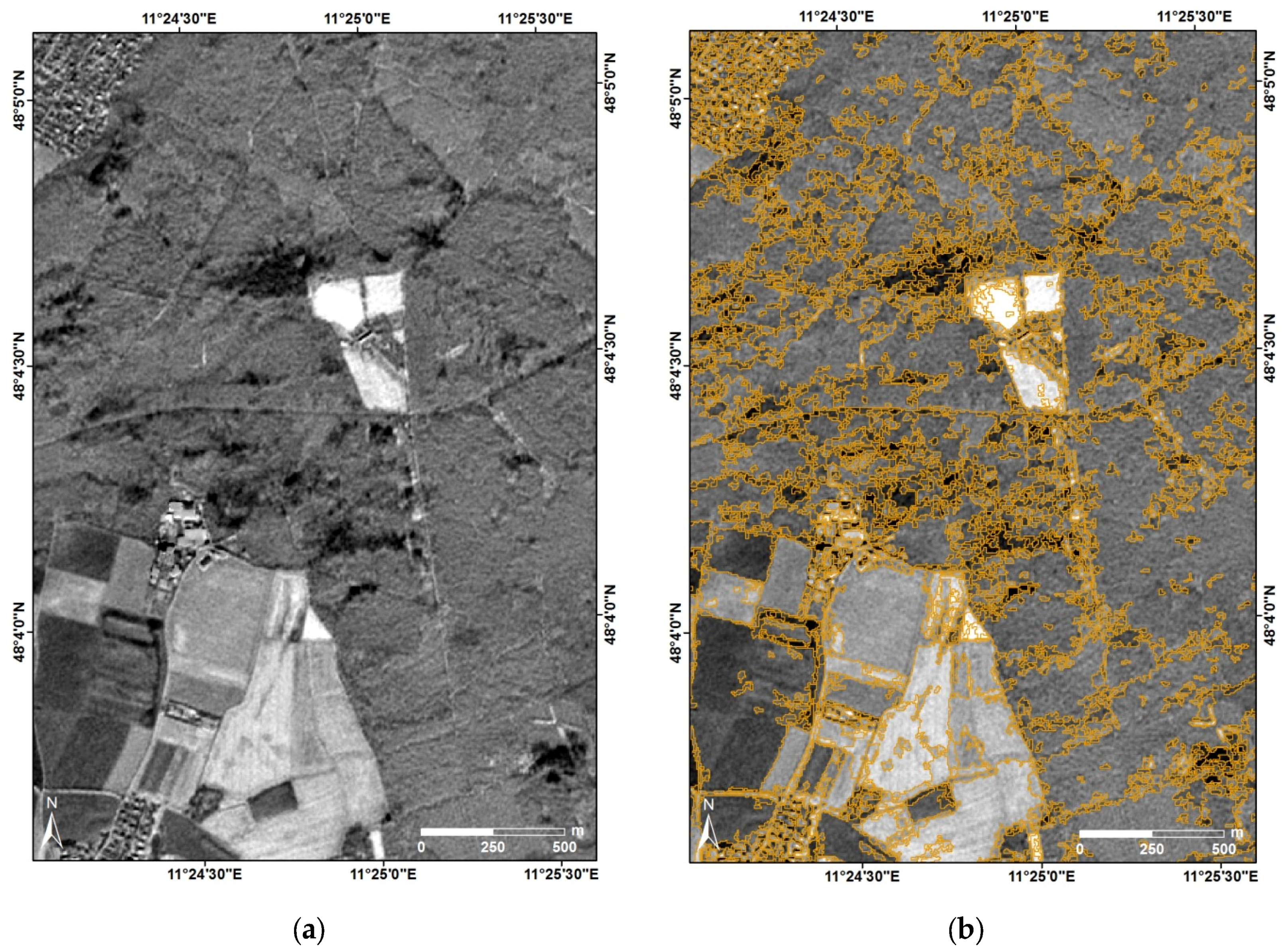
To obtain optimum classification results for windfall change detection, a wide range of predictor layers were analyzed, such as spectral bands, vegetation indices, and texture and statistical measures. In addition, simple band transformations were performed, such as layer differencing, specified Tasseled Cap Transformation (sTCT) [13,37,38], Disturbance Index (DI) [16], Multivariate Alteration Detection (MAD) [39], and Spectral Angle Mapper (SAM) [40] (Figure 2).
At pixel scale, 175 feature layers were generated (Table 5), belonging to three groups: (i) spectral input layers; (ii) transformation-based input layers; and (iii) textural input layers. Additional details are given in Appendix A.
From the 175 input layers of groups (i) to (iii), seventeen statistical measures were calculated per image-object (Table 6), leading to 2975 object variables (175 × 17). For each object, five additional geometrical variables were calculated. These geometrical variables are listed in Table 6. This resulted in 2980 features per bi-temporal image-object.

2.4.2. Segmentation

For image segmentation, the large-scale mean shift (LSMS) algorithm was used [41,42]. LSMS is provided within the Orfeo ToolBox (OTB) 5.0.0 [43]. The mean shift procedure, a non-parametric clustering, was originally proposed by Fukunaga and Hostetler [44]. For image segmentation, the pre- and post-storm images were trimmed. Extreme values (beneath 0.5 percentile and above 99.5 percentile of all pixel values) were removed and images were linearly rescaled to values between 0 and 255.
LSMS requires the setting of three parameters: spatial radius (hs), range radius (hr), and minimum region size (ms). hs is the spatial radius of the neighborhood, hr is defining the radius in the multispectral space, and ms the minimum size of generated image objects. If a region is smaller than the ms, the region is merged to the radiometrically closest neighboring object [43].
As we were interested in forest change, we tried to find the best combination of input layers to get objects well delineating changed forest areas. Segmentation tests were performed with both spectral bands and VIs, but we choose to perform the segmentation with spectral bands only. This was done so as not to distort the Random Forest feature selection result, which might otherwise rank the VI high, which was used for segmentation. LSMS was applied to the following layer combinations:
  • stacked pre- and post-storm TOA reflectances (10 layers)
  • difference images of the TOA reflectances (5 layers)
  • difference images of the three spectral channels R, RE, and NIR (3 layers)
  • mean of the three difference images (R, RE, and NIR) (1 layer)
The results were visually compared to the pre- and post-storm images as well as to the orthophotos. The best results were obtained by using one difference layer calculated from the mean of the difference layers R, RE, and NIR (Figure 3). Only this segmentation is considered in the remaining study.
Additional trial-and-error tests (not discussed here) were conducted to assess the optimal settings for hs, hr, and ms. For the test site Munich South, following Boukir et al. [45], we decided to set hs to half the standard deviation (SD) of all image digital numbers and for radiometric radius hr a quarter of the SD was used. Minimum object size (ms) was set to 10 pixels (250 m2), representing a small group of trees (see Table 7).
For Landsberg, these values had to be adjusted to take into account the finer granularity of the forest cover. The best segmentation result was obtained by setting hs to a third of SD and hr to a sixth of the SD of the image digital numbers. ms has been set to five pixels (125 m2), since the forest is more mixed (and more heterogeneous) compared to the Munich South area.
To reduce the amount of data in the subsequent analysis, only objects that were located within forests were kept. For this purpose, a forest mask was used [46]. The mask was buffered with 10 m to possibly capture windfall areas on the edge of the forest mask.

2.5. Object-Based Change Detection for Detecting Windthrow Areas ≥0.5 ha

2.5.1. Random Forest Classifier

For the classification and feature selection we used the Random Forest (RF) classifier [47]. This machine learning algorithm consists of an ensemble of decision trees and is currently widely used in remote sensing [25,27,48,49,50]. RF was chosen for classification as the algorithm can deal with few training data, multi-modal classes, and non-normal data distributions [47,51]. Some further advantages of RF are the included bootstrapping which provides the relatively unbiased “out-of-bag” (OOB) classification results and the calculation of feature important measures such as Mean Decrease in Accuracy (MDA). This important ranking can be used for feature selection [29,50,52,53]. More details about the algorithm can be found in Pal [54], Hastie et al. [51], and Immitzer et al. [55].
In this study we used the RF implementation randomForest [56] in R 3.2.3 [57]. For the modelling we set the number of trees to be grown in the run (ntree) to 1000. The number of features used in each split (mtry) was set equal to the square root of the total number of input features [47,56].

2.5.2. Training Data

For the training of the supervised RF classifier, 25 reference polygons for class “windthrow” had been manually selected in the RapidEye imagery. In addition, 25 polygons representing the class “non-windthrow” were selected, such as intact forest, water bodies, fields, shadows, and urban areas. Examples are provided in Figure 4. The RF classifier is sensitive to the number of input data, but as we did not know the amount of windthrow areas, we chose to have equal proportions of training data in the two classes.

2.5.3. Feature Selection

To reduce the number of features in the final RF model, we started with a model including all input features and made a step-wise reduction by removing each time the least important variable based on the MDA values [50,53,58]. MDA importance values were recalculated at each step. At the end, the model with the lowest number of input features which reached min 97.5% of the maximum OOB overall accuracy was used.

2.5.4. Classification Margin

Besides indicating the most voted class of each object (majority vote), the frequency of the most common and the second most common class was calculated. By subtracting these two values, a measure for classification reliability can be derived [29,50,59]. In case that the RF model is certain about the class assignment, most trees will be classified in the same class. Consequently, this will result in a high difference of the classification frequency compared to the second voted class. In the same logic, if two classes are more or less equally often assigned to a given object, the difference is low, indicating a small confidence.
After classification, for each as ‘windthrow’ classified image-object the classification security was calculated and grouped in five classes (see Table 8). The regrouping of results permits in a subsequent step to merge adjacent polygons belonging to the same security class.

2.6. Pixel-Based Change Detection for Identifying Smaller Groups of Fallen Trees

To identify changes smaller than the smallest segment defined by ms (Table 7)—less than 250 m2 for Munich South and 125 m2 for Landsberg—a pixel-based classification was performed. We intended to do so to provide the foresters an additional map at hand, which they could use to faster detect small-scale damage (e.g., some few individual or clusters of damaged trees). This is important because in the region we often had problems with the undetected damaged trees providing nesting material for subsequent bark beetle infestations.
For this, only the two most important predictor layers of the RF model were used as input data. Therefore, the layers with the highest number of counts (several statistical metrics) were chosen among those highest ranked in the RF feature selection. Correlated variables can influence accuracy importance measures (like MDA or mean decrease in Gini (MDG)), but are able to deliver reliable results; MDA is more stable when correlations among the predictor variables exist [55].
Different CD methods have been tested, which are fast and relatively easy applicable, such as difference images, SAM and MAD. The best results were achieved with a combination of SAM and MAD, yielding satisfactory results also in areas with haze and shadows. For this purpose, MAD and also SAM was calculated on each of the layer stacks of the two most important variables of the pre- and post-storm images. The two generated MAD layers and the generated SAM layer were then joined to form a layer stack of three change layers.

2.7. Validation

The quality of the object-based change detection was evaluated against the validation data set (see Table 5). Contingency matrices were calculated for the two binary variables, distinguishing between four possibilities [60,61]:
  • True positives (tp): windthrow areas are correctly detected
  • False positives (fp): unchanged objects are incorrectly flagged as “windthrow”
  • True negatives (tn): unchanged objects are correctly identified as “no change”
  • False negatives (fn): windthrow areas are incorrectly flagged as “no change”
The case “true negatives” did not apply in our analysis since only windthrow areas have been digitized in the validation data set.
From the contingency matrix, we calculated sensitivity (Equation (1)) [62]. Sensitivity, also known as true positive rate, is defined as:
Sensitivity = tp ( tp + fn )
This criterion indicates the percentage of segments that have been properly classified as windthrow area, subject to the totality of all by the algorithm recognized windfalls.
For the pixel-based approach, visual validation with the orthophotos was conducted, since it was not possible to map all single fallen trees in the test areas.

3. Results and Discussion

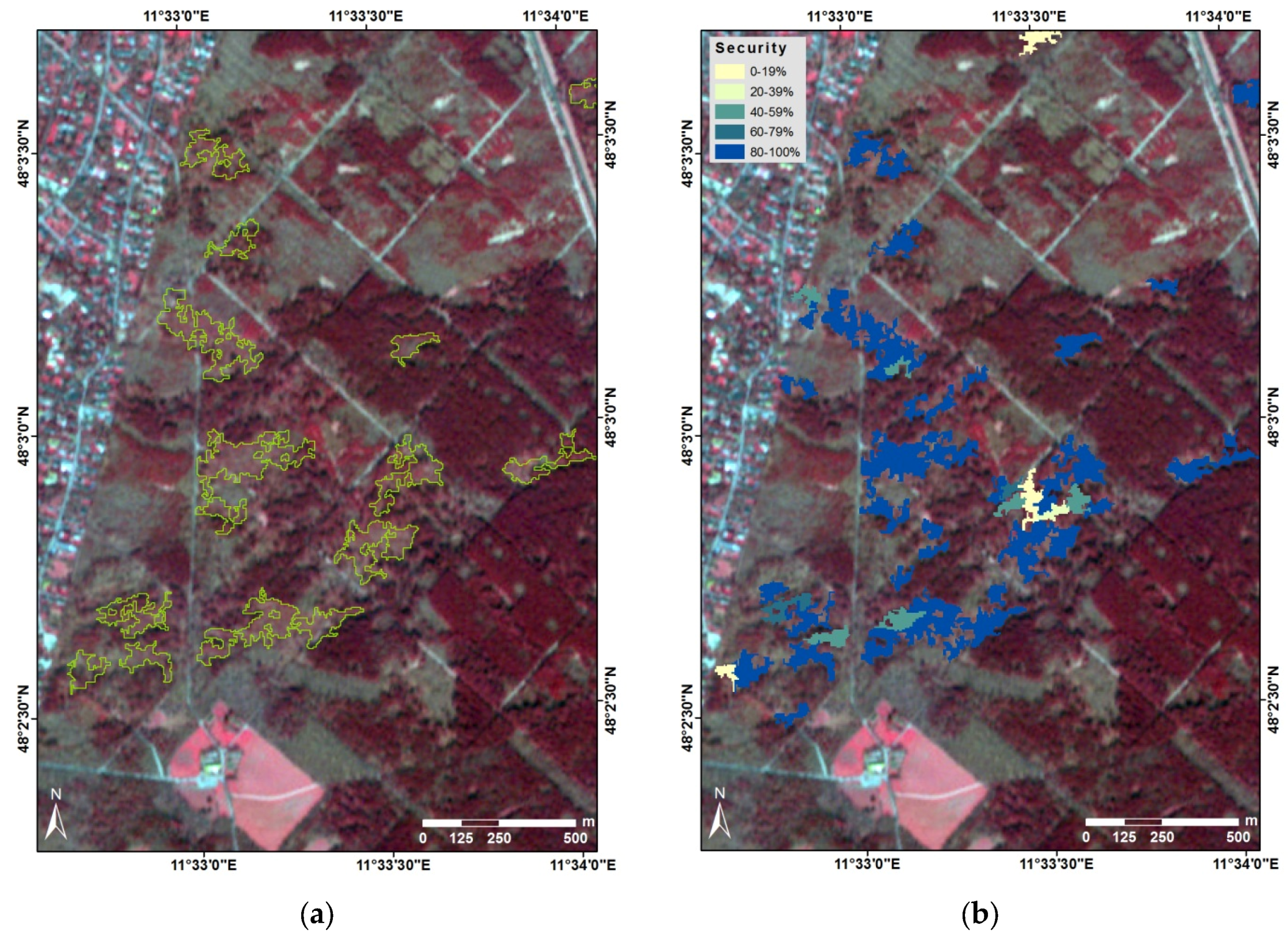
3.1. Detection of Windthrow Areas ≥0.5 ha Using Object-Based Classification

3.1.1. Classification Results

The results of the object-based windthrow detection for areas greater than 0.5 ha were satisfactory. An exemplary change detection result of the study site Munich South is shown in Figure 5. The contingency table for the study site Munich South is given in Table 9.
Sensitivity for the test area Munich South was 93%, indicating a high conformity between the classified windfalls and the validation data set. The detected windthrow areas also showed a good surface sharpness. Of the 295 areas 71% were almost congruent (with size deviations between 1 and 3 m), 13% of the surfaces were smaller in size than the actual windfall extent, 15% were larger in size. Twenty-four areas were wrongly classified as windfall. These areas often belonged to security classes 1 or 2 (see Table 8), and were often adjacent to bright gravel pits or to fallow grounds. This indicates that misclassification was mainly caused by over-exposure from neighboring bright areas.
Similar results were obtained for the Landsberg area; validation results for areas larger than 0.5 ha are listed in Table 9. The sensitivity for this second area was 96%, thereby demonstrating a good match between the classified windthrow areas and the validation data. The detected windthrow areas had a good congruency, however, they were less good than for the Munich South study site. Approximately 51% had an overlapping extent, 47% of the detected areas were smaller than the validation areas, and 2% were larger.
The reason for underestimating the extent of the detected areas is probably caused by the acquisition date of the orthophotos. They were acquired four months after the storm event. Therefore, the actual windfall areas could not be identified perfectly. Instead, what was mapped corresponds to the forest state at the time of orthophotos acquisition. At that time, some of the damaged areas were already cleared. The cleared sites were often greater than the actual affected area, due to additional timber outtake for protective measures. This was also confirmed by visual inspection of RapidEye and Google Earth images [63], which were acquired closer to the storm event—these images reveal a better agreement.
In Landsberg, only one area was incorrectly classified as windfall, whereas four windthrow areas were not detected. These areas were mainly mixed forest stands with a relatively strong increase in vegetation cover coupled with the release of understory [64] and the onset of spring and during the 32 days between the storm event and image acquisition.

3.1.2. Selected Features

Not all features were equally important for the detection of windthrow areas using the RF model. The nine most important variables for the Munich South study area are listed in Table 10. Four of the selected variables were directly based on the Plant Senescence Reflectance Index (PSRI); a fifth one (RE reflectance) entered into the calculation of PSRI. Two of the remaining selected variables were associated with the NIR channel of the pre-storm image. The last variable was based on Haralick texture.
The strong contribution of PSRI is interesting because the index had been initially developed to determine the onset of senescence and to monitor the vegetation’s vitality [65]. In our study, PRSI was found to be very important in detecting forest disturbances caused by windfalls. This demonstrates the suitability of the index and the RE channels for the detection of stressed and damaged vegetation.
Besides the PSRI, the NIR band of the post-storm image was selected twice among the important features. As PSRI is calculated with bands of the visible spectra (B, R, and RE) and does not consider the NIR region, it is sensitive to plant pigments. NIR reflectance provides information about the cell structure of the plant and is widely used in vegetation monitoring [66]. The post-NIR reflectance indicated changes in leaf structure of the damaged trees.
Similar to the Munich South area, the PSRI was found to be one of the most important variables for the Landsberg area, and the variables based on RE reflectance appeared several times (Table 11). The RE channel of the pre-storm image was ranked highest. Three variables were based on the difference of Normalized Difference Red Edge Blue Index, also closely related to the RE channel. Only the variable difference of 2nd Modified Soil Adjusted Vegetation Index was based on NIR channel (see Table 11). No texture measure was observed to be amongst the most important variables.
Together, Table 10 (Munich South) and Table 11 (Landsberg) show that mainly vegetation indices and spectral bands were important for windthrow detection. Specified Tasseled Cap Coefficients (sTCC) and DI features were not selected, indicating that these transformations perform better with sensors they originally have been developed for, such as, sensors with shortwave infrared (SWIR) bands (e.g., Landsat). Textural features are in principle suitable for object-based change detection [67], but played a minor role compared to the variables based on spectral information.

3.2. Detection of Smaller Groups of Fallen Trees Using Pixel-Based Change Detection

For the pixel-based CD, the key input layers of the RF feature selection, PSRI and NIR (see Table 10) were used. In this MAD-SAM combination, both the larger windfalls as well as smaller windfall patches appear in blue (Figure 6). To test the applicability of the pixel-based approach, the MAD-SAM combination was accordingly computed for the Landsberg study area and led to similar results as those observed for Munich South.
Visual comparison of the change images with orthophotos and validation data was conducted. Figure 6, Figure 7 and Figure 8 illustrate the result of the PBA approach. The utilized layer combination also shows single fallen trees. Furthermore, the PBA is fast to compute.
Applying SAM and MAD yields better results in comparison to a simple layer stack of the selected features in the areas covered by haze. Since MAD [39] and SAM, given the same number of bands [68], can handle data acquired with different sensors, this approach could be suitable if there is no pre- and post-storm image available from the same sensor, or if a cloud free scene was acquired faster by a different sensor. However, this case is subject to further research.

3.3. Quantification of Forest Loss

Significant forest cover loss was detected in both study areas. In the Munich South region spruce monoculture stands were primarily affected by storm fall. The main damage pattern observed was in the form of smaller canopy gaps. Only a few forest areas larger than two hectares were disturbed (see Figure 9).
Most of the damage in Munich South occurred in the western and northern part of the study area. The damage happened often, but not only, in forests where canopy gaps already existed. These canopy gaps were present for different reasons, like forest thinning (in these areas often skid roads are visible) and forest conversion. The forest conversion is done to adapt the forest to the local conditions and to minimize windthrow damage as well as biotic damage (Bavarian State Institute of Forestry: personal communication), changing the forest type from spruce monoculture to mixed forest. Furthermore, the area was hit by winter storms Elon and Felix in January 2015, which caused minor damage compared to storm Niklas. Less forest damage occurred in the southeastern part of the study area (see Figure 10), which had less canopy gaps.In the Landsberg study area mostly spruce and mixed forests were affected. Overall, this region was also affected by windfall, but the individual windthrow patches showed smaller sizes as in Munich South (see Figure 9). In both study sites, mainly smaller areas, with a size up to 0.9 ha were blown down. Only a few areas were larger than 2.0 ha. Often these areas were closely located to each other, only being separated through a group of remaining trees.
The windthrow detection performed well for both flat conditions (e.g., Munich South) and in hilly terrain (e.g., Landsberg). In mountainous areas, however, the classification outcome is expected to be less accurate, as illumination conditions may vary sharply between adjacent sites. Difficulties are also expected regarding the detection of damaged leaning trees. In our test sites, the spectral differences between leaning trees and intact trees were only minor, prohibiting reliable results.
Both data sets featured the effects of snow, shadows, and haze. Despite these difficult conditions, the algorithms could identify practically all windthrow areas with good area sharpness. Shadow had minor influence in the pixel-based analysis. This demonstrates that the methods are robust enough for handling difficult and varying conditions during image acquisition as long as the area is not covered by clouds.

3.4. Comparisson with Other Studies

Our findings correlate with other studies applying HR [12] and VHR satellite data [14] for windthrow change detection. Chehata et al. [12] implemented an object-based approach using HR Formosat-2 data on a 60 km2 study site to detect windthrow. In Chehata et al.’s study, 87.8% of the disturbed areas were identified, with green band shown to be the most useful. It should be noted that Formosat-2 does not have a red edge band. The study performed by Elatawneh et al. [14] detected forest cover loss with OBCD after a windfall with accuracies ranging between 87% and 96% on a 130 km2 area. RapidEye data were applied, and the red edge band was labeled as best performing band, as a result of a visual pre-study [69]. However, our study included two larger test sites (720 km2 and 840 km2) compared to the studies by Chehata et al. [12] and Elatawneh et al. [14] and various predictor variables (texture, spectral, statistical, and geometrical) were used to test for windthrow detection with Random Forest.
NDVI is widely used for vegetation and disturbance monitoring. However, in our study, the NDVI was not ranked highly as a suitable predictor layer. This is in line with studies applying HR or VHR for both disturbance [12,14] and severity [7] detection after windthrow. This further confirms the findings of other studies [5,6,17] that used medium resolution data for forest disturbances monitoring.
Some uncertainties exist in our study. First, we used two RapidEye datasets with 23 and 32 days of difference, and we performed our analysis under the explicit assumption that the changes we discovered were mainly caused by windthrow, due to the narrow time window. As salvage logging is the common harvesting type in our study region, we cannot, however, exclude the possibility that some of the detected changes were caused by forest thinnings, which would present similar spectral changes [7]. Secondly, we focused only on the detection of changed forest areas. The scope of our study did not consider the identification of several different types of land change, like in other studies [9,21]. In the future, different types of disturbances should be included in the approach. Further, while the impact of changes in illumination and phenology between pre- and post-storm images in our study were minor, they could generally lead to misinterpretations.

4. Conclusions

In our study, we applied a two-step approach to identify windthrow areas in a temperate forest. To detect damaged areas greater than 0.5 ha, we developed an object-based method using Random Forest (RF) classification that demonstrated high accuracies, which were validated with independent reference data. The built-in feature selection identified similar predictor variables in both areas. After having identified the most important input layers, as derived from the object-based approach, we developed the subsequent pixel-based method to visualize windthrow areas on pixel level. With this, we intended to give the foresters an additional map to have at hand, which they could use to faster detect small-scale damage (e.g., just some few damaged trees or canopy gaps). This is important because in the past, problems occurred with undetected clusters of damaged trees which provided breeding material for bark beetles.
Our study proved the applicability and robustness of RF classifier for windthrow detection at object- and pixel-level and its benefit for ranking features according to their importance. As RF is easy to implement and to handle, we recommend its use for windthrow detection.
According to our results, vegetation indices proved suitable measures for the detection of windthrow. In particular, vegetation indices achieved better results compared to individual spectral bands or texture. Plant Senescence Reflectance Index (PSRI) and Normalized Difference Red Edge Blue Index (NDREDI), both applying the red edge and blue spectral bands, were identified as the most applicable indices. The use of sensor data providing information in red edge and blue spectral bands, and vegetation indices including those bands, is therefore potentially beneficial, but any definite suggestion would require further research under different test conditions. In future work, the use of high resolution Sentinel-2 data is potentially beneficial for windthrow detection. However, it needs to be tested whether small-scale changes can be captured with the Sentinel-2 data, which have a coarser resolution than RapidEye. Otherwise, Sentinel-2, especially considering its three red edge bands as well as its shortwave infrared bands, has the necessary spectral band setting to perform well in large-scale windthrow monitoring. Our developed method as well as existing forest disturbance monitoring methods based on Landsat data need to be further tested with Sentinel-2 data.

Acknowledgments

The project ‘Fast Response’ was funded by the German Federal Ministry of Economic Affairs and Energy by grant number 50EE1314 and Bavarian State Ministry for Food, Agriculture and Forestry. The authors thank the Bavarian State Forest enterprise and the Austrian State Forest Enterprise for their cooperation. We also thank the students from Technical University of Munich, Inken Dirks and Constantin Freiherr von Thielmann, as well as Ruben Goldstayn for their assistance. The authors further acknowledge the open source community. The following open source software was used: Orfeo ToolBox (www.orfeo-toolbox.org), QGIS 2.8 (http://qgis.osgeo.org), and R 3.1.2 (http://CRAN.R-project.org).

Author Contributions

K.E. conceived and designed the experiments, K.E., M.I., and S.B. performed the experiments, O.B. and A.S. conducted fieldwork, O.B. supervised the collection of reference data, K.E. analyzed the data, K.E. wrote the manuscript, M.I. and C.A. revised draft versions of the manuscript. All authors revised the final manuscript.

Conflicts of Interest

The authors declare no conflict of interest.

Appendix A

Appendix A.1. Vegetation Indices

Vegetation indices (VIs) are mathematical combinations of spectral bands enhancing a specific spectral behavior of the plants [4,23,70]. Numerous VIs exist assessing various aspects of the vegetation cover (e.g., water content, plant senescence, leaf chlorophyll content). We calculated eighteen different VIs as potential candidates for the identification of forest windthrow disturbances (see Table A1).
Table A1. Vegetation indices used for the change detection analysis.
IndexEquationReference
Atmospherically Resistant Vegetation Index A R V I = N I R ( 2 × R B ) N I R + ( 2 × R B ) [71]
Difference Difference Vegetation Index D D = ( 2 × N I R R ) ( G B ) [72]
Difference Vegetation Index D V I = N I R R [73]
Enhanced Vegetation Index E V I 2 = 2.5 × ( N I R R ) ( N I R + ( 2.4 × R + 1.0 ) ) [74]
Green Atmospherically Resistant Vegetation Index G A R I = NIR ( G ( B R ) ) NIR + ( G ( B R ) ) [75]
Green Normalized Difference Vegetation Index G N D V I = N I R G N I R + G [76]
Infrared Percentage Vegetation Index I P V I = N I R N I R + R [77]
2nd Modified Soil Adjusted Vegetation Index M S A V I 2 = 2 × NIR + 1 ( 2 × N I R + 1 ) 2 8 × ( NIR R ) 2 [78]
Normalized Difference Red Edge Index N D R E I = N I R R E G N I R + R E G [79,80]
Normalized Difference Greenness Index N D G I = G R G + R [81]
Normalized Difference Red Edge Blue Index N D R E G B = R E G B R E G + B evolved for this study
Normalized Difference Vegetation Index N D V I = N I R R N I R + R [82]
Normalized Near Infrared N N I R = N I R ( N I R + R + G ) [83]
Plant Senescence Reflectance Index P S R I = R B R E G [65]
Red Edge Normalized Difference Vegetation Index R E G   N D V I = R E G R R E G + R [84]
Red Edge Ratio Index 1 R R I 1 = N I R R E G [85]
Ratio Vegetation Index R V I = N I R R [86,87]
Soil Adjusted Vegetation Index S A V I = 1.5 × ( N I R R ) N I R + R + 0.5 [88]

Appendix A.2. Tasseled Cap Transformation and Disturbance Index

The Tasseled Cap Transformation (TCT) is an orthogonal spectral feature space transformation originally derived for Landsat data [37,89]. TCT reduces multi-spectral bands into three (relatively) uncorrelated features, the so-called Tasseled Cap Coefficients (TCC)—Brightness (B), Greenness (G), and Wetness (W).
From the TCC, Healey et al. [16] derived a measure for quantifying forest disturbance (Equation (A1)), the Disturbance Index (DI):
DI = B − (G − W)
The DI is assuming that in disturbed forest areas, brightness will rise and at the same time, greenness and moisture content will decrease [16]. Positive DI values therefore indicate forest disturbances.
Since TCT is sensor specific [90] and RapidEye has no shortwave infrared band (SWIR) like Landsat, we applied specific transformations developed for RapidEye [13,38]. Specific TCC (sTCC) were calculated following both approaches. Subsequently, DIs were computed, as well as difference layers (before/after the storm). After visual inspection of the derived DI images, it turned out that the DIs responded strongly to haze present in the post-storm images. Thus, a modified DI was calculated, only subtracting G from B, not taking the third sTCC into account.

Appendix A.3. Image Differencing

Image differencing is a simple and well-established CD approach [4,26,91]. In our study, difference layers were calculated for all spectral bands, vegetation indices, texture layers, Tasseled Cap Coefficients, and Disturbance Indices by subtracting the post-storm values from the pre-storm values.

Appendix A.4. Spectral Angle Mapper

In the Spectral Angle Mapper approach (SAM), the spectral similarity between two spectral signatures is quantified by calculating the spectral angle in the n-dimensional feature space [40]. SAM is applied both in hyperspectral remote sensing [92,93] as well as in multispectral CD [68,94]. Any change over time leads to higher angles, since the pixel vectors vary more compared to unchanged pixels. The advantage of this method is the relatively high robustness to brightness differences between two acquisitions [95]. A moving window was applied using a radius of 5, 10, 15, and 20 m from the initial pixel. SAM was calculated once with the pre-image being the master image, once with the post-image for the four different radii.

Appendix A.5. Multivariate Alteration Detection

Multivariate Alteration Detection (MAD) minimizes the correlation between two data sets and maximizes the data’s variance [39]. The method is based on standard canonical correlation analysis, which transforms the input images into two multivariate vector sets. Subsequently, linear combinations of the multivariate sets are built, so-called canonical variates [39]. The lower order variates contain the higher variance. The change is detected by differencing the two sets of uncorrelated canonical variates, generating uncorrelated MAD components.

Appendix A.6. Textural Features

Texture, the spatial micro-variation of images grey-levels, can enhance the results of object-based image classifications, as demonstrated in several forest applications [53,96,97]. An undisturbed forest has a more homogenous texture compared to a disturbed forest. Single fallen or small groups of damaged trees will especially lead to higher variation in texture.
We applied multi-scale (Wavelet transformation) and statistical (Haralick and Grey-Level Run-Length features) textural measures. The various textural features are summarized in Table A2.
Table A2. Summary of textural features used in the study.
HaralickGrey-Level Run-Length Matrix
Energy
Entropy
Correlation
Inverse Difference Moment
Inertia
Cluster Shade
Cluster Prominence
Haralick Correlation
[98]Short Run Emphasis
Long Run Emphasis
Grey-Level Nonuniformity
Run Length Nonuniformity
Run Percentage
[99]
Low Grey-Level Run Emphasis
High Grey-Level Run Emphasis
[100]
Short Run Low Grey-Level Emphasis
Short Run High Grey-Level Emphasis
Long Run Low Grey-Level Emphasis
Long Run High Grey-Level Emphasis
[101]
The multi-scale wavelet transformation [102] decomposes the grey-level frequencies of an image into images of different scales [67]. For each scale, four new sub-images are calculated: approximation and three directions (horizontal, vertical, and diagonal). The low-frequency approximation sub-image is needed to calculate the next scale. The three direction sub-images give high-frequency information about image texture details. We applied a discrete stationary wavelet transformation with Coiflets (coif1) [53] at four different scales. After the fourth scale a natural convergence occurs, therefore only four transformation passages were performed [103]. To reduce the data amount, the mean of the three directions was calculated for each level, assuming no preferred direction of windthrow patterns. The transformations were computed with MATLAB 8.2.0.29 [104].
In addition, eight second order Haralick texture features were calculated based on grey-level co-occurrence matrix (GLCM) [98] (Table A2). The computation was carried out with OTB, which uses a variation of GLCM for faster processing [43].
Furthermore, eleven higher statistical order texture features based on Grey-Level Run Length-Matrices (GLRLM) were calculated in OTB [43] (Table A2). GLRLM measures the runs of pixels with the same grey-level values in a set direction [99].
All textural features were calculated for the five spectral channels of the pre- and post-storm images, as well as the wavelet layers for NDVI. Textural change layers were derived by subtracting the pre-storm feature from the post-storm features [105].

Appendix A.7. Geometrical Characteristics

For each image object, five additional geometrical characteristics were calculated: area, perimeter as well as compactness [106], shape index and fractal dimension [107].

References

  1. Schelhaas, M.-J.; Nabuurs, G.-J.; Schuck, A. Natural disturbances in the European forests in the 19th and 20th Centuries. Glob. Chang. Biol. 2003, 9, 1620–1633. [Google Scholar] [CrossRef]
  2. Seidl, R.; Schelhaas, M.-J.; Rammer, W.; Verkerk, P.J. Increasing forest disturbances in Europe and their impact on carbon storage. Nat. Clim. Chang. 2014, 4, 806–810. [Google Scholar] [CrossRef] [PubMed]
  3. Seidl, R.; Rammer, W. Climate change amplifies the interactions between wind and bark beetle disturbances in forest landscapes. Landsc. Ecol. 2016, 1–14. [Google Scholar] [CrossRef]
  4. Coppin, P.R.; Bauer, M.E. Digital change detection in forest ecosystems with remote sensing imagery. Remote Sens. Rev. 1996, 13, 207–234. [Google Scholar] [CrossRef]
  5. Vogelmann, J.E.; Tolk, B.; Zhu, Z. Monitoring forest changes in the southwestern United States using multitemporal Landsat data. Remote Sens. Environ. 2009, 113, 1739–1748. [Google Scholar] [CrossRef]
  6. Wang, F.; Xu, Y.J. Comparison of remote sensing change detection techniques for assessing hurricane damage to forests. Environ. Monit. Assess. 2010, 162, 311–326. [Google Scholar] [CrossRef] [PubMed]
  7. Rich, R.L.; Frelich, L.; Reich, P.B.; Bauer, M.E. Detecting wind disturbance severity and canopy heterogeneity in boreal forest by coupling high-spatial resolution satellite imagery and field data. Remote Sens. Environ. 2010, 114, 299–308. [Google Scholar] [CrossRef]
  8. Jonikavičius, D.; Mozgeris, G. Rapid assessment of wind storm-caused forest damage using satellite images and stand-wise forest inventory data. iForest 2013, 6, 150–155. [Google Scholar] [CrossRef]
  9. Baumann, M.; Ozdogan, M.; Wolter, P.T.; Krylov, A.; Vladimirova, N.; Radeloff, V.C. Landsat remote sensing of forest windfall disturbance. Remote Sens. Environ. 2014, 143, 171–179. [Google Scholar] [CrossRef]
  10. Immitzer, M.; Atzberger, C. Early detection of bark beetle infestation in Norway Spruce (Picea abies, L.) using WorldView-2 data. Photogramm. Fernerkund. Geoinform. 2014, 2014, 351–367. [Google Scholar] [CrossRef]
  11. Latifi, H.; Fassnacht, F.E.; Schumann, B.; Dech, S. Object-based extraction of bark beetle (Ips typographus L.) infestations using multi-date LANDSAT and SPOT satellite imagery. Prog. Phys. Geogr. 2014, 38, 755–785. [Google Scholar] [CrossRef]
  12. Chehata, N.; Orny, C.; Boukir, S.; Guyon, D.; Wigneron, J.P. Object-based change detection in wind storm-damaged forest using high-resolution multispectral images. Int. J. Remote Sens. 2014, 35, 4758–4777. [Google Scholar] [CrossRef]
  13. Arnett, J.T.T.R.; Coops, N.C.; Gergel, S.E.; Falls, R.W.; Baker, R.H. Detecting stand replacing disturbance using RapidEye imagery: A tasseled cap transformation and modified disturbance index. Can. J. Remote Sens. 2014, 40, 1–14. [Google Scholar] [CrossRef]
  14. Elatawneh, A.; Wallner, A.; Manakos, I.; Schneider, T.; Knoke, T. Forest cover database updates using multi-seasonal RapidEye data—Storm event assessment in the Bavarian forest national park. Forests 2014, 5, 1284–1303. [Google Scholar] [CrossRef]
  15. Schwarz, M.; Steinmeier, C.; Holecz, F.; Stebler, O.; Wagner, H. Detection of Windthrow in mountainous regions with different remote sensing data and classification methods. Scand. J. For. Res. 2003, 18, 525–536. [Google Scholar] [CrossRef]
  16. Healey, S.; Cohen, W.; Zhiqiang, Y.; Krankina, O. Comparison of Tasseled Cap-based Landsat data structures for use in forest disturbance detection. Remote Sens. Environ. 2005, 97, 301–310. [Google Scholar] [CrossRef]
  17. Desclée, B.; Bogaert, P.; Defourny, P. Forest change detection by statistical object-based method. Remote Sens. Environ. 2006, 102, 1–11. [Google Scholar] [CrossRef]
  18. Dyukarev, E.A.; Pologova, N.N.; Golovatskaya, E.A.; Dyukarev, A.G. Forest cover disturbances in the South Taiga of West Siberia. Environ. Res. Lett. 2011, 6, 035203. [Google Scholar] [CrossRef]
  19. Zhu, Z.; Woodcock, C.E.; Olofsson, P. Continuous monitoring of forest disturbance using all available Landsat imagery. Remote Sens. Environ. 2012, 122, 75–91. [Google Scholar] [CrossRef]
  20. Negrón-Juárez, R.; Baker, D.B.; Zeng, H.; Henkel, T.K.; Chambers, J.Q. Assessing hurricane-induced tree mortality in U.S. Gulf Coast forest ecosystems. J. Geophys. Res. Biogeosci. 2010, 115, G04030. [Google Scholar] [CrossRef]
  21. Hermosilla, T.; Wulder, M.A.; White, J.C.; Coops, N.C.; Hobart, G.W. Regional detection, characterization, and attribution of annual forest change from 1984 to 2012 using Landsat-derived time-series metrics. Remote Sens. Environ. 2015, 170, 121–132. [Google Scholar] [CrossRef]
  22. Chen, G.; Hay, G.J.; Carvalho, L.M.T.; Wulder, A. Object-based change detection. Int. J. Remote Sens. 2012, 33, 4434–4457. [Google Scholar] [CrossRef]
  23. Hussain, M.; Chen, D.; Cheng, A.; Wei, H.; Stanley, D. Change detection from remotely sensed images: From pixel-based to object-based approaches. ISPRS J. Photogramm. Remote Sens. 2013, 80, 91–106. [Google Scholar] [CrossRef]
  24. Hecheltjen, A.; Thonfeld, F.; Menz, G. Recent advances in remote sensing change detection—A review. In Land Use and Land Cover Mapping in Europe; Manakos, I., Braun, M., Eds.; Springer: Dordrecht, The Netherlands, 2014; pp. 145–178. [Google Scholar]
  25. Bovolo, F.; Bruzzone, L. The time variable in data fusion: A change detection perspective. IEEE Geosci. Remote Sens. Mag. 2015, 3, 8–26. [Google Scholar] [CrossRef]
  26. Tewkesbury, A.P.; Comber, A.J.; Tate, N.J.; Lamb, A.; Fisher, P.F. A critical synthesis of remotely sensed optical image change detection techniques. Remote Sens. Environ. 2015, 160, 1–14. [Google Scholar] [CrossRef]
  27. Li, X.; Cheng, X.; Chen, W.; Chen, G.; Liu, S. Identification of forested landslides using LiDAR data, object-based image analysis, and machine learning algorithms. Remote Sens. 2015, 7, 9705–9726. [Google Scholar] [CrossRef]
  28. Wu, X.; Yang, F.; Roly, L. Land cover change detection using texture analysis. J. Comput. Sci. 2010, 6, 92–100. [Google Scholar] [CrossRef]
  29. Immitzer, M.; Vuolo, F.; Atzberger, C. First experience with Sentinel-2 data for crop and tree species classifications in Central Europe. Remote Sens. 2016, 8, 1–27. [Google Scholar] [CrossRef]
  30. Schumacher, P.; Mislimshoeva, B.; Brenning, A.; Zandler, H.; Brandt, M.; Samimi, C.; Koellner, T. Do red edge and texture attributes from high-resolution satellite data improve wood volume estimation in a Semi-arid mountainous region? Remote Sens. 2016, 8, 540. [Google Scholar] [CrossRef]
  31. Ramoelo, A.; Skidmore, A.K.; Cho, M.A.; Schlerf, M.; Mathieu, R.; Heitkönig, I.M.A. Regional estimation of savanna grass nitrogen using the red-edge band of the spaceborne RapidEye sensor. Int. J. Appl. Earth Obs. Geoinform. 2012, 19, 151–162. [Google Scholar] [CrossRef]
  32. Clevers, J.G.P.W.; Kooistra, L. Retrieving canopy chlorophyll content of potato crops using Sentinel-2 bands. In Proceedings of ESA Living Planet Symposium, Edinburgh, UK, 9–13 September 2012; pp. 1–8.
  33. Haeseler, S.; Lefebvre, C. Hintergrundbericht: Orkantief NIKLAS wütet am 31. März 2015 über Deutschland 2015; Deutscher Wetterdienst (DWD), Climate Data Center(CDC): Offenbach am Main, Germany, 2015. [Google Scholar]
  34. Preuhsler, T. Sturmschäden in einem Fichtenbestand der Münchener Schotterebene. Allg. Forstz. 1990, 46, 1098–1103. [Google Scholar]
  35. BlackBridge. Satellite Imagery Product Specifications; Version 6.1; BlackBridge: Berlin, Germany, 2015. [Google Scholar]
  36. Vicente-Serrano, S.; Pérez-Cabello, F.; Lasanta, T. Assessment of radiometric correction techniques in analyzing vegetation variability and change using time series of Landsat images. Remote Sens. Environ. 2008, 112, 3916–3934. [Google Scholar] [CrossRef]
  37. Kauth, J.; Thomas, G.S. The tasselled cap—A graphic description of the spectral-temporal development of agricultural crops as seen by LANDSAT. In Symposium on Machine Processing of Remotely Sensed Data; Institute of Electrical and Electronics Engineers: West Lafayette, IN, USA, 1976; pp. 41–51. [Google Scholar]
  38. Schönert, M.; Weichelt, H.; Zillmann, E.; Jürgens, C. Derivation of tasseled cap coefficients for RapidEye data. In Earth Resources and Environmental Remote Sensing/GIS Applications V, 92450Q; Michel, U., Schulz, K., Eds.; SPIE: Bellingham, WA, USA, 2014; Volume 9245, pp. 1–11. [Google Scholar]
  39. Nielsen, A.A.; Conradsen, K.; Simpson, J.J. Multivariate Alteration Detection (MAD) and MAF Postprocessing in Multispectral, Bitemporal Image Data: New approaches to change detection studies. Remote Sens. Environ. 1998, 64, 1–19. [Google Scholar] [CrossRef]
  40. Kruse, F.A.F.; Lefkoff, A.B.; Boardman, J.W.; Heidebrecht, K.B.; Shapiro, A.T.; Barloon, P.J.; Goetz, A.F.H. The spectral image processing system (SIPS)-interactive visualization and analysis of imaging spectrometer data. Remote Sens. Environ. 1993, 44, 145–163. [Google Scholar] [CrossRef]
  41. Comaniciu, D.; Meer, P. Mean shift: A robust approach toward feature space analysis. IEEE Trans. Pattern Anal. Mach. Intell. 2002, 24, 603–619. [Google Scholar] [CrossRef]
  42. Michel, J.; Youssefi, D.; Grizonnet, M. Stable mean-shift algorithm and its application to the segmentation of arbitrarily large remote sensing images. IEEE Trans. Geosci. Remote Sens. 2015, 53, 952–964. [Google Scholar] [CrossRef]
  43. Orfeo ToolBox (OTB) Development Team. The Orfeo ToolBox Cookbook, A Guide for Non-Developers; Updated for OTB-5.2.1; CNES: Paris, France, 2016. [Google Scholar]
  44. Fukunaga, K.; Hostetler, L. The estimation of the gradient of a density function, with applications in pattern recognition. IEEE Trans. Inf. Theory 1975, 21, 32–40. [Google Scholar] [CrossRef]
  45. Boukir, S.; Jones, S.; Reinke, K. Fast mean-shift based classification of very high resolution images: Application to forest cover mapping. In Proceedings of the ISPRS Annals of the Photogrammetry, Remote Sensing and Spatial Information Sciences, Melbourne, Australia, 25 August–1 September 2012; Volume I-7, pp. 293–298.
  46. Arbeitsgemeinschaft der Vermessungsverwaltung der Länder der Bundesrepublik Deutschland (AdV). Amtliches Topographisch-Kartographisches Informationssystem (ATKIS). Available online: http://www.adv-online.de/AAA-Modell/ATKIS/ (accessed on 7 January 2016).
  47. Breiman, L. Random forests. Mach. Learn. 2001, 45, 5–32. [Google Scholar] [CrossRef]
  48. Immitzer, M.; Stepper, C.; Böck, S.; Straub, C.; Atzberger, C. Use of WorldView-2 stereo imagery and National Forest Inventory data for wall-to-wall mapping of growing stock. For. Ecol. Manag. 2016, 359, 232–246. [Google Scholar] [CrossRef]
  49. Ng, W.-T.; Meroni, M.; Immitzer, M.; Böck, S.; Leonardi, U.; Rembold, F.; Gadain, H.; Atzberger, C. Mapping Prosopis spp. with Landsat 8 data in arid environments: Evaluating effectiveness of different methods and temporal imagery selection for Hargeisa, Somaliland. Int. J. Appl. Earth Obs. Geoinform. 2016, 53, 76–89. [Google Scholar] [CrossRef]
  50. Schultz, B.; Immitzer, M.; Formaggio, A.R.; Sanches, I.D.A.; Luiz, A.J.B.; Atzberger, C. Self-guided segmentation and classification of multi-temporal Landsat 8 images for crop type mapping in Southeastern Brazil. Remote Sens. 2015, 7, 14482–14508. [Google Scholar] [CrossRef]
  51. Hastie, T.; Tibshirani, R.; Friedman, J. The Elements of Statistical Learning: Data Mining, Inference, and Prediction, 2nd ed.; Springer: New York, NY, USA, 2009. [Google Scholar]
  52. Genuer, R.; Poggi, J.-M.; Tuleau-Malot, C. Variable selection using random forests. Pattern Recognit. Lett. 2010, 31, 2225–2236. [Google Scholar] [CrossRef]
  53. Toscani, P.; Immitzer, M.; Atzberger, C. Texturanalyse mittels diskreter Wavelet Transformation für die objektbasierte Klassifikation von Orthophotos. Photogramm. Fernerkund. Geoinform. 2013, 2, 105–121. [Google Scholar] [CrossRef]
  54. Pal, M. Random forest classifier for remote sensing classification. Int. J. Remote Sens. 2005, 26, 217–222. [Google Scholar] [CrossRef]
  55. Immitzer, M.; Atzberger, C.; Koukal, T. Tree species classification with Random Forest using very high spatial resolution 8-band WorldView-2 satellite data. Remote Sens. 2012, 4, 2661–2693. [Google Scholar] [CrossRef]
  56. Liaw, A.; Wiener, M. Classification and regression by randomForest. R News 2002, 2, 18–22. [Google Scholar]
  57. R Core Team. R: A Language and Environment for Statistical Computing; R Foundation for Statistical Computing: Vienna, Austria, 2016. [Google Scholar]
  58. Granitto, P.M.; Furlanello, C.; Biasioli, F.; Gasperi, F. Recursive feature elimination with random forest for PTR-MS analysis of agroindustrial products. Chemom. Intell. Lab. Syst. 2006, 83, 83–90. [Google Scholar] [CrossRef]
  59. Vuolo, F.; Atzberger, C. Improving land cover maps in areas of disagreement of existing products using NDVI time series of MODIS—Example for Europe. Photogramm. Fernerkund. Geoinform. 2014, 393–407. [Google Scholar] [CrossRef]
  60. Rosin, P.L.; Ioannidis, E. Evaluation of global image thresholding for change detection. Pattern Recognit. Lett. 2003, 24, 2345–2356. [Google Scholar] [CrossRef]
  61. Radke, R.J.; Andra, S.; Al-Kofahi, O.; Roysam, B. Image change detection algorithms: A systematic survey. IEEE Trans. Image Process. 2005, 14, 294–307. [Google Scholar] [CrossRef] [PubMed]
  62. Dorko, G.; Schmid, C. Selection of scale-invariant parts for object class recognition. In Proceedings of the Ninth IEEE International Conference on Computer Vision, Nice, France, 13–16 October 2003; pp. 634–640.
  63. Google Inc. Google Earth 2015. Available online: https://google.com/earth/ (accessed on 10 April 2015).
  64. Peterson, C.J. Catastrophic wind damage to North American forests and the potential impact of climate change. Sci. Total Environ. 2000, 262, 287–311. [Google Scholar] [CrossRef]
  65. Merzlyak, M.N.; Gitelson, A.A.; Chivkunova, O.B.; Rakitin, V. Non-destructive optical detection of pigment changes during leaf senescence and fruit ripening. Physiol. Plant. 1999, 106, 135–141. [Google Scholar] [CrossRef]
  66. Ollinger, S.V. Sources of variability in canopy reflectance and the convergent properties of plants. New Phytol. 2011, 189, 375–394. [Google Scholar] [CrossRef] [PubMed]
  67. Ruiz, L.A.; Fernández-Sarría, A.; Recio, J.A. Texture feature extraction for classification of remote sensing data using wavelet decomposition: A comparative study. In Proceedings of the 20th ISPRS Congress, Istanbul, Turkey, 12–23 July 2004; pp. 1109–1114.
  68. Carvalho, O.A.J.; Guimarães, R.F.; Gillespie, A.R.; Silva, N.C.; Gomes, R.A.T. A new approach to change vector analysis using distance and similarity measures. Remote Sens. 2011, 3, 2473–2493. [Google Scholar] [CrossRef]
  69. Elatawneh, A.; Rappl, A.; Schneider, T.; Knoke, T. A semi-automated method of forest cover losses detection using RapidEye images: A case study in the Bavarian forest National Park. In Proceedings of the 4th RESA Workshop, Neustrelitz, Germany, 21–22 March 2012; Borg, E., Ed.; GITO Verlag für industrielle Informationstechnik und Organisation: Neustrelitz, Germany, 2012; pp. 183–200. [Google Scholar]
  70. Baig, M.H.A.; Zhang, L.; Shuai, T.; Tong, Q. Derivation of a tasselled cap transformation based on Landsat 8 at-satellite reflectance. Remote Sens. Lett. 2014, 5, 423–431. [Google Scholar] [CrossRef]
  71. Kaufman, Y.J.; Tanre, D. Atmospherically resistant vegetation index (ARVI) for EOS-MODIS. IEEE Trans. Geosci. Remote Sens. 1992, 30, 261–270. [Google Scholar] [CrossRef]
  72. Jackson, R.D.; Slater, P.N.; Pinter, P.J. Discrimination of growth and water stress in wheat by various vegetation indices through clear and turbid atmospheres. Remote Sens. Environ. 1983, 13, 187–208. [Google Scholar] [CrossRef]
  73. Tucker, C.J. Red and photographic infrared linear combinations for monitoring vegetation. Remote Sens. Environ. 1979, 8, 127–150. [Google Scholar] [CrossRef]
  74. Jiang, Z.; Huete, A.R.; Didan, K.; Miura, T. Development of a two-band enhanced vegetation index without a blue band. Remote Sens. Environ. 2008, 112, 3833–3845. [Google Scholar] [CrossRef]
  75. Gitelson, A.A.; Kaufman, Y.J.; Merzlyak, M.N. Use of a green channel in remote sensing of global vegetation from EOS-MODIS. Remote Sens. Environ. 1996, 58, 289–298. [Google Scholar] [CrossRef]
  76. Gitelson, A.A.; Merzlyak, M.N. Signature analysis of leaf reflectance spectra: Algorithm development for remote sensing of chlorophyll. J. Plant Physiol. 1996, 148, 494–500. [Google Scholar] [CrossRef]
  77. Crippen, R. Calculating the vegetation index faster. Remote Sens. Environ. 1990, 34, 71–73. [Google Scholar] [CrossRef]
  78. Qi, J.; Kerr, Y.; Chehbouni, A. External factor consideration in vegetation index development. In Proceedings of the 6th Symposium on Physical Measurements and Signatures in Remote Sensing, Val D’Isere, France, 17–21 January 1994; pp. 723–730.
  79. Gitelson, A.; Merzlyak, M.N. Spectral reflectance changes associated with autumn senescence of Aesculus hippocastanum L. and Acer platanoides L. leaves. Spectral features and relation to chlorophyll estimation. J. Plant Physiol. 1994, 143, 286–292. [Google Scholar] [CrossRef]
  80. Barnes, E.M.E.; Clarke, T.R.T.; Richards, S.E.S.; Colaizzi, P.D.D.; Haberland, J.; Kostrzewski, M.; Waller, P.; Choi, C.; Riley, E.; Thompson, T.; et al. Coincident detection of crop water stress, nitrogen status and canopy density using ground-based multispectral data. In Proceedings of the Fifth International Conference on Precision Agriculture, Bloomington, MN, USA, 16–19 July 2000; Robert, P.C., Rust, R.H., Larson, W.E., Eds.; American Society of Agronomy: Madison, WI, USA, 2000. [Google Scholar]
  81. Chamard, P.; Courel, M.-F.; Guenegou, M.; Lerhun, J.; Levasseur, J.; Togola, M. Utilisation des bandes spectrales du vert et du rouge pour une meilleure évaluation des formations végétales actives. In Télédétection et Cartographie; AUPELF-UREF, Réseau Télédétection Journées scientifiques; Presses de l’université du Québec: Québec, CA, 1991; pp. 203–209. [Google Scholar]
  82. Rouse, J.; Haas, R.; Schell, J.; Deering, D. Monitoring vegetation systems in the Great Plains with ERTS. In Proceedings of the Third ERTS Symposium; National Aeronautics and Space Administration: Washington, DC, USA, 1974; Volume 351, pp. 309–317. [Google Scholar]
  83. Sripada, R.P.; Heiniger, R.W.; White, J.G.; Meijer, A.D. Aerial color infrared photography for determining early in-season nitrogen requirements in corn. Agron. J. 2006, 98, 968–977. [Google Scholar] [CrossRef]
  84. ApolloMapping. Using RapidEye 5-meter Imagery for Vegetation Analysis; ApolloMapping: Boulder, CO, USA, 2012. [Google Scholar]
  85. Ehammer, A.; Fritsch, S.; Conrad, C.; Lamers, J.; Dech, S. Statistical derivation of fPAR and LAI for irrigated cotton and rice in arid Uzbekistan by combining multi-temporal RapidEye data and ground measurements. In Remote Sensing for Agriculture, Ecosystems, and Hydrology XII; Neale, C.M.U., Maltese, A., Eds.; SPIE: Bellingham, WA, USA, 2010; Volume 7824, pp. 1–10. [Google Scholar]
  86. Jordan, C.F. Derivation of leaf area index from quality of light on the forest floor. Ecology 1969, 50, 663–666. [Google Scholar] [CrossRef]
  87. Pearson, R.; Miller, L. Remote mapping of standing crop biomass for estimation of the productivity of the short-grass Prairie, Pawnee National Grasslands, Colorado. In Proceedings of the 8th International Symposium on Remote Sensing of Environment, Ann Arbor, MI, USA, 2–6 October 1972; pp. 1357–1381.
  88. Huete, A.R. A soil-adjusted vegetation index (SAVI). Remote Sens. Environ. 1988, 25, 295–309. [Google Scholar] [CrossRef]
  89. Crist, E.P.; Cicone, R.C. A physically-based transformation of Thematic Mapper data—The TM Tasseled Cap. IEEE Trans. Geosci. Remote Sens. 1984, GE-22, 256–263. [Google Scholar] [CrossRef]
  90. Yarbrough, L.; Easson, G.; Kuszmaul, J.S. Tasseled cap coefficients for the QuickBird2 sensor: A comparison of methods and development. In Proceedings of the PECORA 16 Conference on Global priorities in land remote sensing, American Society for Photogrammetry and Remote Sensing, Sioux Falls, SD, USA, 23–27 October 2005; pp. 23–27.
  91. Singh, A. Review Article Digital change detection techniques using remotely-sensed data. Int. J. Remote Sens. 1989, 10, 989–1003. [Google Scholar] [CrossRef]
  92. Cho, M.A.; Debba, P.; Mathieu, R.; Naidoo, L.; van Aardt, J.; Asner, G.P. Improving discrimination of savanna tree species through a multiple-endmember spectral angle mapper approach: Canopy-level analysis. IEEE Trans. Geosci. Remote Sens. 2010, 48, 4133–4142. [Google Scholar] [CrossRef]
  93. Einzmann, K.; Ng, W.-T.; Immitzer, M.; Pinnel, N.; Atzberger, C. Method analysis for collecting and processing in-situ hyperspectral needle reflectance data for monitoring Norway Spruce. Photogramm. Fernerkund. Geoinform. 2014, 5, 423–434. [Google Scholar] [CrossRef]
  94. Carvalho, O.A.J.; Guimarães, R.F.; Silva, N.C.; Gillespie, A.R.; Gomes, R.A.T.; Silva, C.R.; De Carvalho, A.P. Radiometric normalization of temporal images combining automatic detection of pseudo-invariant features from the distance and similarity spectral measures, density scatterplot analysis, and robust regression. Remote Sens. 2013, 5, 2763–2794. [Google Scholar] [CrossRef]
  95. Schlerf, M.; Hill, J.; Bärisch, S.; Atzberger, C. Einfluß der spektralen und räumlichen Auflösung von Fernerkundungsdaten bei der Nadelwaldklassifikation. Photogramm. Fernerkund. Geoinform. 2003, 2003, 25–34. [Google Scholar]
  96. Tuominen, S.; Pekkarinen, A. Performance of different spectral and textural aerial photograph features in multi-source forest inventory. Remote Sens. Environ. 2005, 94, 256–268. [Google Scholar] [CrossRef]
  97. Beguet, B.; Guyon, D.; Boukir, S.; Chehata, N. Automated retrieval of forest structure variables based on multi-scale texture analysis of VHR satellite imagery. ISPRS J. Photogramm. Remote Sens. 2014, 96, 164–178. [Google Scholar] [CrossRef]
  98. Haralick, R.M.; Shanmugam, K.; Dinstein, I. Textural features for image classification. IEEE Trans. Syst. Man Cybern. 1973, 3, 610–621. [Google Scholar] [CrossRef]
  99. Galloway, M.M. Texture analysis using gray level run lengths. Comput. Graph. Image Process. 1975, 4, 172–179. [Google Scholar] [CrossRef]
  100. Chu, A.; Sehgal, C.M.; Greenleaf, J.F. Use of gray value distribution of run lengths for texture analysis. Pattern Recognit. Lett. 1990, 11, 415–420. [Google Scholar] [CrossRef]
  101. Dasarathy, B.V.; Holder, E.B. Image characterizations based on joint gray level-run length distributions. Pattern Recognit. Lett. 1991, 12, 497–502. [Google Scholar] [CrossRef]
  102. Mallat, S.G. A theory for multiresolution signal decomposition: The wavelet representation. IEEE Trans. Pattern Anal. Mach. Intell. 1989, 11, 674–693. [Google Scholar] [CrossRef]
  103. Ouma, Y.O.; Ngigi, T.G.; Tateishi, R. On the optimization and selection of wavelet texture for feature extraction from high-resolution satellite imagery with application towards urban-tree delineation. Int. J. Remote Sens. 2006, 27, 73–104. [Google Scholar] [CrossRef]
  104. The MathWorks Inc. MATLAB; Version 8.2.0.29 (r2013b); The MathWorks Inc.: Natick, MA, USA, 2013. [Google Scholar]
  105. Klonus, S.; Tomowski, D.; Ehlers, M.; Reinartz, P.; Michel, U. Combined edge segment texture analysis for the detection of damaged buildings in crisis areas. IEEE J. Sel. Top. Appl. Earth Obs. Remote Sens. 2012, 5, 1118–1128. [Google Scholar] [CrossRef]
  106. Osserman, R.; Yau, S.T. The Isoperimetric inequality. Bull. Am. Math. Soc. 1978, 84, 1182–1238. [Google Scholar] [CrossRef]
  107. Krummel, J.R.; Gardner, R.H.; Sugihara, G.; O’Neill, R.V.; Coleman, P.R. Landscape patterns in a disturbed environment. Oikos 1987, 48, 321–324. [Google Scholar] [CrossRef]
Figure 1. False color composites of RapidEye scenes (band combination: near infrared—red—green) acquired after storm Niklas covering the two test sites Munich South (east) and Landsberg (west) in Bavaria, Germany.
Forests 08 00021 g001
Figure 2. Flowchart of the developed windthrow analysis procedure. Input features for Random Forest are highlighted (orange). Abbreviations: TOA (Top Of Atmosphere correction), VI (Vegetation Indices), MAD (Multivariate Alteration Detection), SAM (Spectral Angel Mapper), TCC (Tasseled Cap Coefficients), DI (Disturbance Index), LSMS (Large-scale Mean Shift), NDVI (Normalized Difference Vegetation Index), NIR (Near Infrared), R (Red), and RE (Red Edge).
Forests 08 00021 g002
Figure 3. Detail of Munich South scene showing input (a) and resulting image segmentation (b). The input layer (a) consists of the mean values of the three difference layers from red, red edge, and near infrared bands. Darker regions within the forested area indicate windthrow.
Forests 08 00021 g003
Figure 4. Example reference polygons showing different windthrow areas (yellow polygons) as well as non-windthrow polygons (green polygons). Polygons are overlaid on a false color composite orthophoto (band combination: near infrared—red—green) acquired four months after the storm.
Forests 08 00021 g004
Figure 5. Object-based change detection results for an exemplary area in Munich South. Polygons are overlaid on false color composite of post-storm scene (band combination: near infrared—red—green). (a) Reference windthrow areas greater than 0.5 ha; (b) detected windthrow areas greater than 0.25 ha, the minimum mapping unit of the segmentation, with classification margins.
Forests 08 00021 g005
Figure 6. Detail of false color composite (band combination: near infrared—red—green) pre-storm RapidEye scene (a); post-storm RapidEye scene (b) and pixel-based change detection result based on RapidEye data (c) for Munich South. Windthrow areas appear in blue.
Forests 08 00021 g006
Figure 7. Examples of detected windthrow areas depicted with false color composite orthophoto (band combination: near infrared—red—green) (a,c,e) and pixel-based result based on RapidEye data (b,d,f) for Munich South. Windthrow areas appear in blue. Scattered tree damage (ad), the damage often occurred in recently thinned forest (a) where skid trails are visible. Small groups of affected trees could also be detected (e,f). Here small thrown stands, comprising eight (left) and three (right) trees, respectively, were detected.
Forests 08 00021 g007
Figure 8. Example of single thrown trees for the Munich South study site (a) false color composite orthophoto scene (band combination: near infrared—red—green) showing remaining trees (tree shadows) and thrown trees (dead trees with root plates); (b) Pixel-based results based on RapidEye data where single fallen trees appear in blue.
Forests 08 00021 g008
Figure 9. Frequency of size distribution of windthrow affected areas ≥0.5 ha for Munich South (Left) and Landsberg (Right) resulting from the object-based approach.
Forests 08 00021 g009
Figure 10. Occurrence of windthrow areas ≥0.5 ha (green areas) in the Munich South study area. As background is the false color composite (band combination: near infrared—red—green) post-storm RapidEye scene depicted.
Forests 08 00021 g010
Table 1. Selection of essential previous studies for forest disturbance detection. Most studies used medium resolution (deca-metric) satellite data and pixel-based approaches on temperate and boreal forest ecosystems. Abbreviations: TM (Thematic Mapper), ETM+ (Enhanced Thematic Mapper Plus), SPOT (Satellite Pour l’Observation de la Terre), AeS (Aero-Sensing), E-SAR (Experimental airborne SAR), ERS (European Remote Sensing Satellite).
TopicArea (km2)RegionSensorApproachReferences
Forest cover change detection421Minnesota, United StatesLandsat TMDetection of canopy disturbances with vegetation indices, standardized image differencing, and principal component analysisCoppin and Bauer [4]
Monitoring of forest changes with multi-temporal data166New Mexico, United StatesLandsat TM/ETM+Spectral trends of time series data sets to capture forest changesVogelmann et al. [5]
Detection of forest damage resulting from wind storm19,600LithuaniaLandsat TMImage differencing and classification with k-Nearest NeighborJonikavičius and Mozgeris [8]
Forest windfall disturbance detection33,600European Russia; Minnesota, United StatesLandsat TM/ETM+Separation of windfalls and clear cuts with Forestness Index, Disturbance Index, and Tasseled Cap TransformationBaumann et al. [9]
17,100
Object-based change detection to assess wind storm damage60Southwest FranceFormosat-2Automated feature selection process followed by bi-temporal classification to detect wind storm damage in forestsChehata et al. [12]
Windthrow detection in mountainous regions221SwitzerlandIkonos, SPOT-4, Landsat ETM+, AeS-1, E-SAR, ERS-1/2Comparison of active and passive data as well as pixel- and object-based approaches for detecting windthrowSchwarz et al. [15]
Forest disturbance detection3810Washington State, United States; St. Petersburg region, RussiaLandsat TM/ETM+Assessing forest disturbances in multi-temporal data with Tasseled Cap Transformation and Disturbance IndexHealey et al. [16]
4200
5000
Clear-cut detection1800Eastern BelgiumSPOTObject-based image segmentation, image differencing, stochastic analysis of the multispectral signal for clear-cut detectionDesclée et al. [17]
Forest cover disturbance detection32,150West Siberia, RussiaLandsat TM/ETM+Unsupervised classification of Tasseled Cap Indices to detect changes caused by forest harvesting and windthrowDyukarev et al. [18]
Continuous forest disturbance monitoring3600Georgia, United StatesLandsatHigh temporal forest monitoring with Forest Disturbance Algorithm (CMFDA)Zhu et al. [19]
Assessing tree damage caused by hurricanesGolf Coast, United StatesLandsat, MODISEstimating large-scale disturbances by combining satellite data, field data, and modelingNégron-Juárez et al. [20]
Spectral trend analysis to detect forest changes375,000Saskatchewan, CanadaLandsat TM/ETM+Breakpoint analysis of spectral trends with changed objects being attributed to a certain change typeHermosilla et al. [21]
Table 2. Main characteristics of the acquired RapidEye data used to detect windthrow areas caused by storm Niklas on 31 March 2015 in South Bavaria.
Pre-Storm ImagePost-Storm ImageArea
Munich South18 March 201510 April 2015720 km2
Landsberg18 March 201519 April 2015840 km2
Table 3. Number of reference polygons obtained from field surveys per affected forest type. The total area of the reference polygons is also indicated.
Spruce, Pure StandSpruce, Mixed ForestMixed ForestTotal NumberTotal Area (in ha)
Munich South68-1427.5
Landsberg27-43116.6
Table 4. Number of reference polygons (≥0.5 ha) obtained from orthophoto interpretation. The size distribution of the affected windthrow areas is indicated.
Munich SouthLandsberg
Number of polygons307135
Size between 0.5 ≤ 1 ha17693
Size between 1 ≤ 2 ha7932
Size between 2 ≤ 5 ha4610
Size between 5 ≤ 10 ha5-
Size ≤ 10 ha1-
Largest area (in ha)11.54.4
Mean size (in ha)1.31
Total area (in ha)400.8138.6
Table 5. Summary of the 175 available input layers at pixel level, distinguishing between spectral, transformation-based, and textural input layers (more details are given in Appendix A). Abbreviations: VI (Vegetation Indices), MAD (Multivariate Alteration Detection), SAM (Spectral Angel Mapper), sTCC (specified Tasseled Cap Coefficients), DI (Disturbance Index), NDVI (Normalized Difference Vegetation Index), GLRLM (Grey-Level Run-Length Martrix).
Spectral Input LayersTransformation-Based Input LayersTextural Input Layers
Pre-StormPost-StormDifferenceVI DifferencesTCC + DI DifferenceMADSAMWavelet DifferenceHaralick DifferenceGLRLM Difference
B
G
R
RE
NIR
B
G
R
RE
NIR
B
G
R
RE
NIR
18 × VIs3 × sTCC (Annert)5 × 1 layer8 × 1 layer4 scales × 6 (5 spectral and NDVI) mean directions5 × 8 Haralick features5 × 11 GLRLM features
3 × sTCC (Schönert)
2 × DI
2 × sTCB-sTCG
555181058244055
Table 6. Computed statistical and geometrical variables calculated for each image object. The seventeen statistical variables were calculated per input layer (175) whereas only one set of (five) geometrical variables was derived.
StatisticsGeometry
MinimumArea
MaximumPerimeter
MedianCompactness
MeanShape Index
Standard DeviationFractal Dimension
12 percentiles (1 to 99)
Table 7. LSMS segmentation parameters for the two test sites Munich South and Landsberg. The two test sites were segmented using a single layer input image (average of red, red edge, and near infrared channels).
Standard DeviationSpatial Radius hsRange Radius hrMinimum Size ms
Munich South2914.57.2510 (250 m2)
Landsberg22.577.53.755 (125 m2)
Table 8. Overview of the windfall securities classes.
ClassSecurity (in %)
10–19
220–39
340–59
460–79
580–100
Table 9. Contingency table of binary classifier for Munich South and Landsberg.
Munich SouthLandsberg
Reference:
Windthrow
Reference:
No Windthrow
Reference:
Windthrow
Reference:
No Windthrow
Classification result:
windthrow detected
295 (tp)24 (fp)88 (tp)1 (fp)
Classification result:
windthrow not detected
21 (fn)not applicable4 (fn)not applicable
Table 10. Random Forest model with the most important object variables for the Munich South study site. The last column indicates the value of the Mean Decrease in Accuracy (MDA).
IndicatorObject StatisticsMDA
Plant Senescence Reflectance Index difference15 percentile18.5
Plant Senescence Reflectance Index difference5 percentile16.2
Plant Senescence Reflectance Index difference20 percentile15.2
Near Infrared of post-storm image1 percentile14.3
Plant Senescence Reflectance Index difference10 percentile14.1
Red Edge difference25 percentile14.0
Near Infrared of post-storm imageMinimum13.8
Normalized Difference Red Edge Blue Index difference20 percentile13.6
Haralick Correlation of Green difference10 percentile13.2
Table 11. Most important object variables in the Random Forest model for the Landsberg study site. The last column indicates the value of the Mean Decrease in Accuracy (MDA).
IndicatorObject StatisticsMDA
Red Edge of pre-storm imageMaximum21
Normalized Difference Red Edge Blue Index differenceMean19.4
Red Edge difference99 percentile18.4
Normalized Difference Red Edge Blue Index difference75 percentile17.7
Normalized Difference Red Edge Blue Index differenceMedian17.1
2nd Modified Soil Adjusted Vegetation Index difference90 percentile16.8
Plant Senescence Reflectance Index difference75 percentile15.7
Spectral Angle Mapper with radius of 5 neighboring pixel80 percentile15.3

