Article

Monitoring Changes in Water Use Efficiency to Understand Drought Induced Tree Mortality

by
Sparkle L. Malone
1,2
1
Department of Biological Sciences, Florida International University, 11200 S.W. 8th Street, Miami, FL 33199, USA
2
Rocky Mountain Research Station, United States Forest Service, 240 W Prospect Rd., Fort Collins, CO 80526, USA
Forests 2017, 8(10), 365; https://doi.org/10.3390/f8100365
Submission received: 3 August 2017 / Revised: 16 September 2017 / Accepted: 21 September 2017 / Published: 26 September 2017

Abstract

:
Forests are becoming increasingly vulnerable to rising tree mortality rates in response to warming and drought. In California, the most severe drought on record occurred from 2012 to 2016 and high tree mortality rates were observed in response to this prolonged drought. Differences in satellite-derived estimates of water-use efficiency (WUE) under normal (i.e., WUEBASELINE) and drought conditions (ΔWUE = WUE2014 − WUEBASELINE) captured variation in drought resilience, and is used here to understand patterns in tree mortality. Across California forests, a low WUEBASELINE under normal conditions was indicative of a low drought resilience and was associated with increasing tree mortality rates. Forested areas with high drought frequency in recent years (2002–2015) and lower WUEBASELINE were the most vulnerable to high post-drought tree mortality. Post drought tree mortality peaked in 2015 and tree mortality was detected in areas where bark beetles were active. Our results show that spatial and temporal changes in WUE can signal shifts in ecosystem resilience and that water-limited forests are sensitive to temperature- and precipitation-driven drought stress. Considering that forests with low resilience will be poised for dieback in the future if climates continue to feature rising temperatures without compensating increases in precipitation, it is becoming increasingly important that we understand drought vulnerability at the ecosystem level and how it changes over time with climate conditions.

1. Introduction

Rising temperatures combined with drought pose a compounding challenge to tree and forest health [1,2,3]. Of particular concern are potential increases in tree mortality associated with climate-induced physiological stress and interactions with other climate-mediated processes (i.e., insect outbreaks). Even though episodic mortality occurs in the absence of climate change, there is great concern that forests may become increasingly vulnerable to higher background tree mortality rates and large episodic die-offs in response to warming and drought [2,4,5]. Increases in the frequency, duration, and/or severity of drought and heat stress associated with climate change could fundamentally alter the composition, structure, and biogeography of forests [2]. With extreme events projected to become more frequent in the future [6], understanding and predicting the consequences of climate change on forested ecosystems is emerging as a large challenge for scientists [2,3,7].
Evaluating shifts in water use efficiency (WUE) under non-drought and drought conditions provides a good approximation of ecosystem resistance to drought [8]. Defined here as net primary productivity (GPP; g C m−2) per amount of water lost (evapotranspiration: ET; mm m−2), WUE links the biological (i.e., photosynthesis and transpiration) and physical (i.e., evaporation) processes that control carbon and water dynamics. An important measure of ecosystem functionality [9], variation in WUE connotes ecosystem resistance by signaling severe changes in resource availability that lead to shifts in ecosystem function. Here, resistance is the capacity to absorb a disturbance (i.e., drought) and maintain the same function (i.e., productivity) and sensitivity (i.e., WUE) [8,10].
Studies have shown that WUE increases with aridity [8,11,12,13,14,15,16,17] and that water limited ecosystems tend to have higher WUE [11,12,18]. Across all systems, if a drought becomes severe enough, a breakdown in ecosystem resistance can lead to a reduction in WUE [8,14,15,17,19] and ecosystem type conversions [8,17]. A recent study evaluated drought resistance across California ecosystems by quantifying deviations in WUE in 2014 (WUESevere Drought) from WUE under normal climate conditions (WUEBASELINE) [8]. Here, we aim to link shifts in WUE under drought conditions (i.e., ΔWUE = WUESevere Drought − WUEBASELINE) to tree mortality rates to understand at what point severe drought alters the structure and function of forests.
Extended drought has been linked directly to tree mortality in tropical and temperate forests [1,20,21,22] and is indirectly linked to tree mortality by triggering insect or pathogen outbreaks [23,24,25,26,27]. Drought often makes trees more vulnerable to cambium-eating insects and this vulnerability often results in episodes of high tree mortality [23,28]. Small changes in mortality rates can profoundly affect forest structure, composition, and function [29,30,31], making it essential that we improve our understanding of the conditions that enhance tree mortality rates and how mortality varies across the landscape.
The primary objective of this research is to use spatial and temporal patterns in WUE to understand drought induced tree mortality. In California, a prolonged drought occurred from 2012–2016 and high tree mortality rates were observed across forested ecosystems [5]. To enhance our understanding of how forested ecosystems respond to drought and how carbon dynamics change with major shifts in climate and extreme events, we evaluate shifts in WUE across California forests. Here, temporal shifts in WUE is thought to reflect drought induced changes in ecosystem structure and function. We hypothesize that forests with lower WUEBASELINE and ΔWUE will have higher maximum tree mortality rates. The frequency of drought years is also likely to be an important determinant of tree mortality. Studies have shown that a low WUEBASELINE is indicative of low drought resilience [8] and that extended droughts often lead to enhanced tree mortality rates [4]. In California forests, more trees die in years with below normal precipitation, and increases in tree mortality are often evident only for multi-year droughts (2–5 years) [4].
Forests of California are of particular interest because they include the largest and oldest trees on Earth. California relies on forested watersheds to support water provisioning, carbon storage, timber products, ecotourism, and recreation. This is the first study to examine drought induced shifts in WUE using satellite imagery and relate it to tree mortality across forested ecosystems in California. This research is essential to enhancing our understanding of how forested ecosystems respond to drought and how carbon dynamics change with major shifts in climate and extreme events. Climate change projections suggest that extreme droughts will become more frequent in the future [32], making it important that we develop efficient techniques to monitor and quantify changes in ecosystem structure and function.

2. Materials and Methods

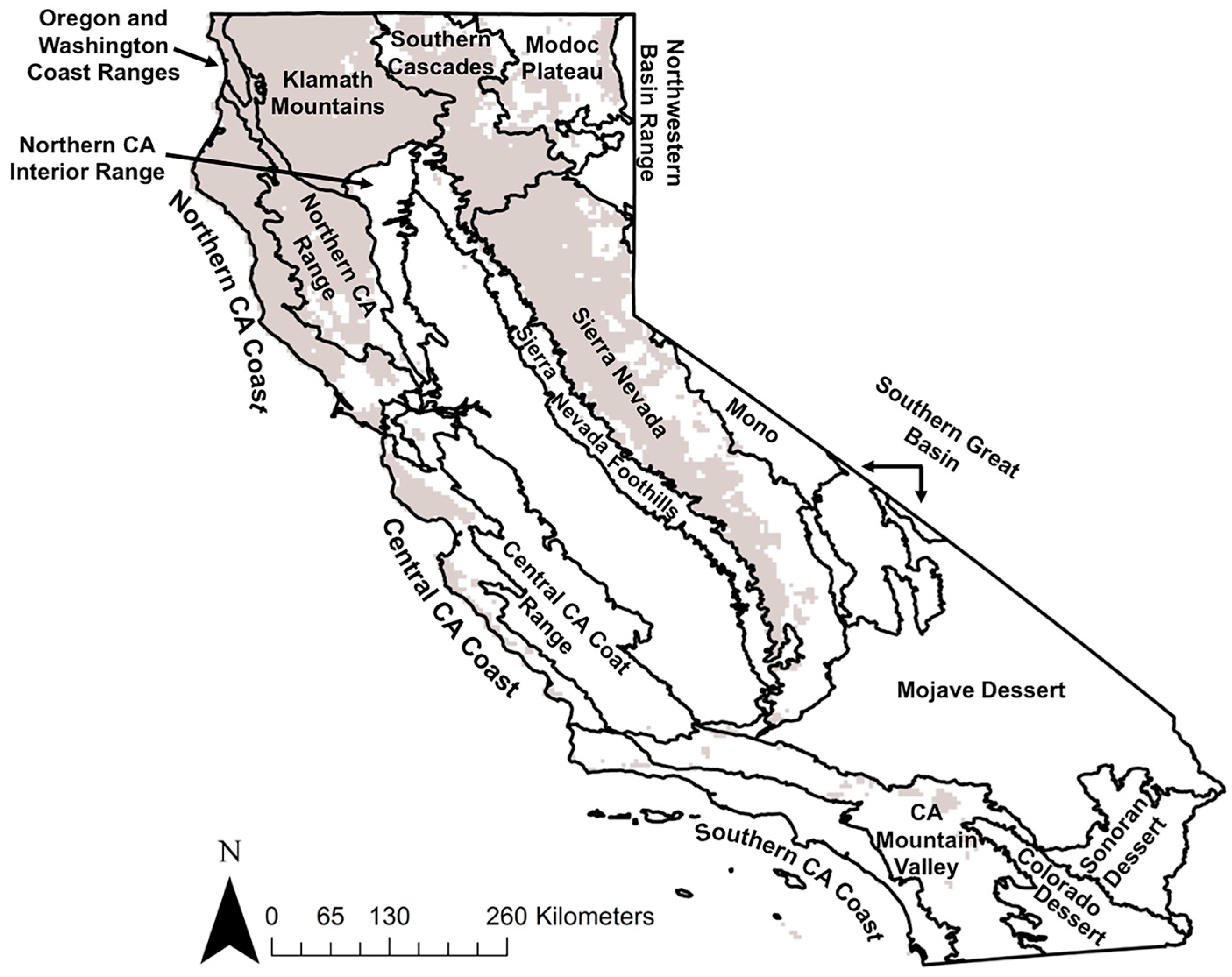
2.1. California Forests

California extends across 20 ecoregions that span the Mediterranean division [33]. Forests occupy nearly a third of the state [34] and most are found in the mountainous areas (i.e., the Klamath, Sierra Nevada, and Coast ranges) and along the state’s north and central coasts (Figure 1). About 58% of forests are dominated by coniferous species: Douglas fir (Pseudotsuga menziesii (Mirb.) Franco), ponderosa pine (Pinus ponderosa Douglas ex C.Lawson), sugar pine (Pinus lamertiana), Jeffrey pine (Pinus jeffreyi Balf.), incense cedar (Cupressaceae calocedrus), white fir (Abies concolor (Gordon) Lindley ex Hildebrand), red fir (Abies magnifica A.Murray), and other true fir species. Hardwood forest types cover an additional 13 million acres (40% of forested land area). The major hardwood forest types are western oak, tanoak/laurel, and other hardwoods. The Moderate Resolution Imaging Spectroradiometer (MODIS) land cover type (MCD12Q1) was used to develop a forest cover layer for the entire state. The most recent annual land cover data available (2012) was used to identify all forested area within the state. Land cover types for forests (evergreen needleleaf, evergreen broadleaf, deciduous needleleaf, deciduous broadleaf, and mixed forests) were dissolved to create a single forest layer (Figure 1). This approach reduces errors associated with classification, which are largely concentrated among classes (i.e., forests) that encompass ecological and biophysical gradients [35].

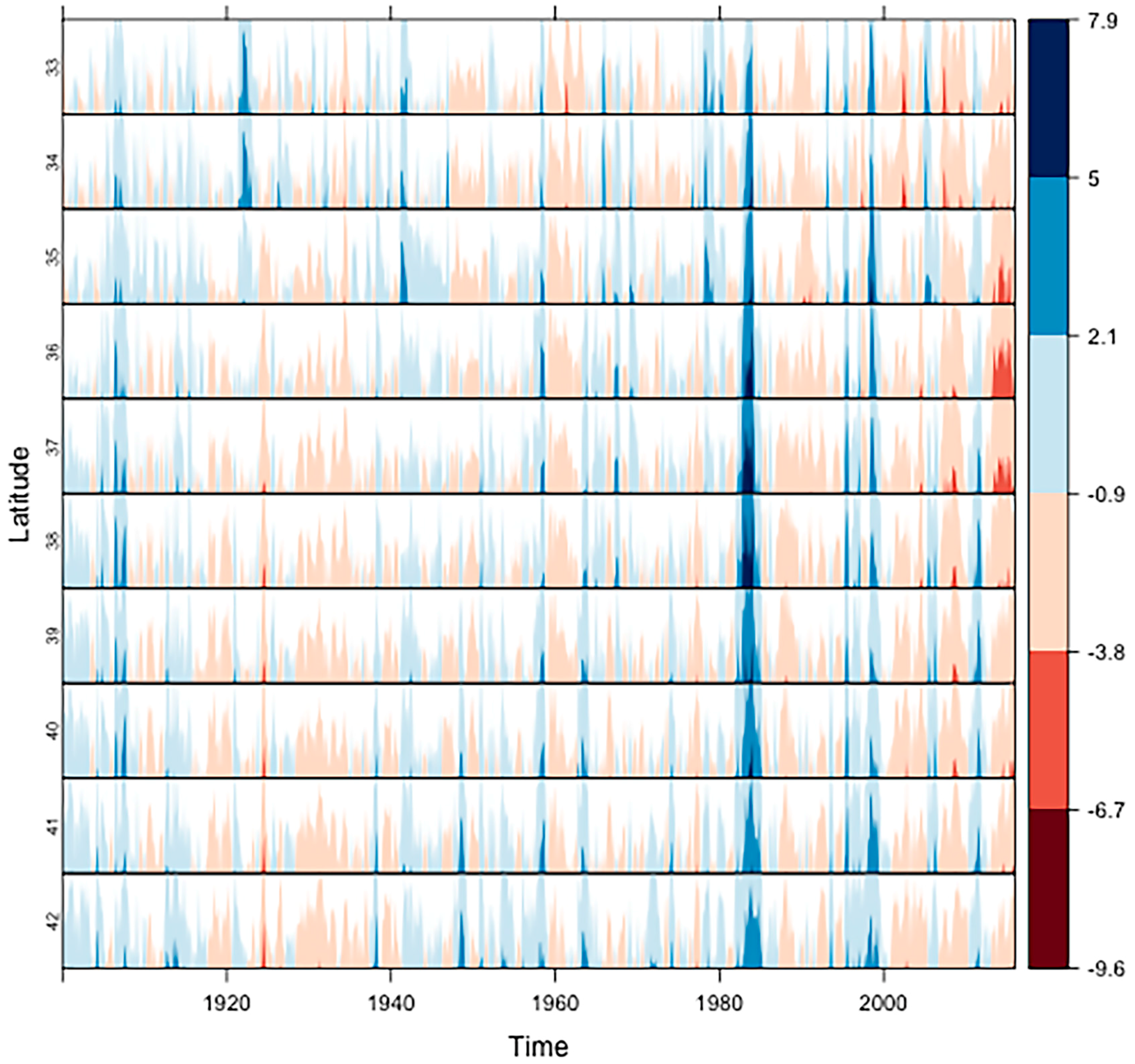
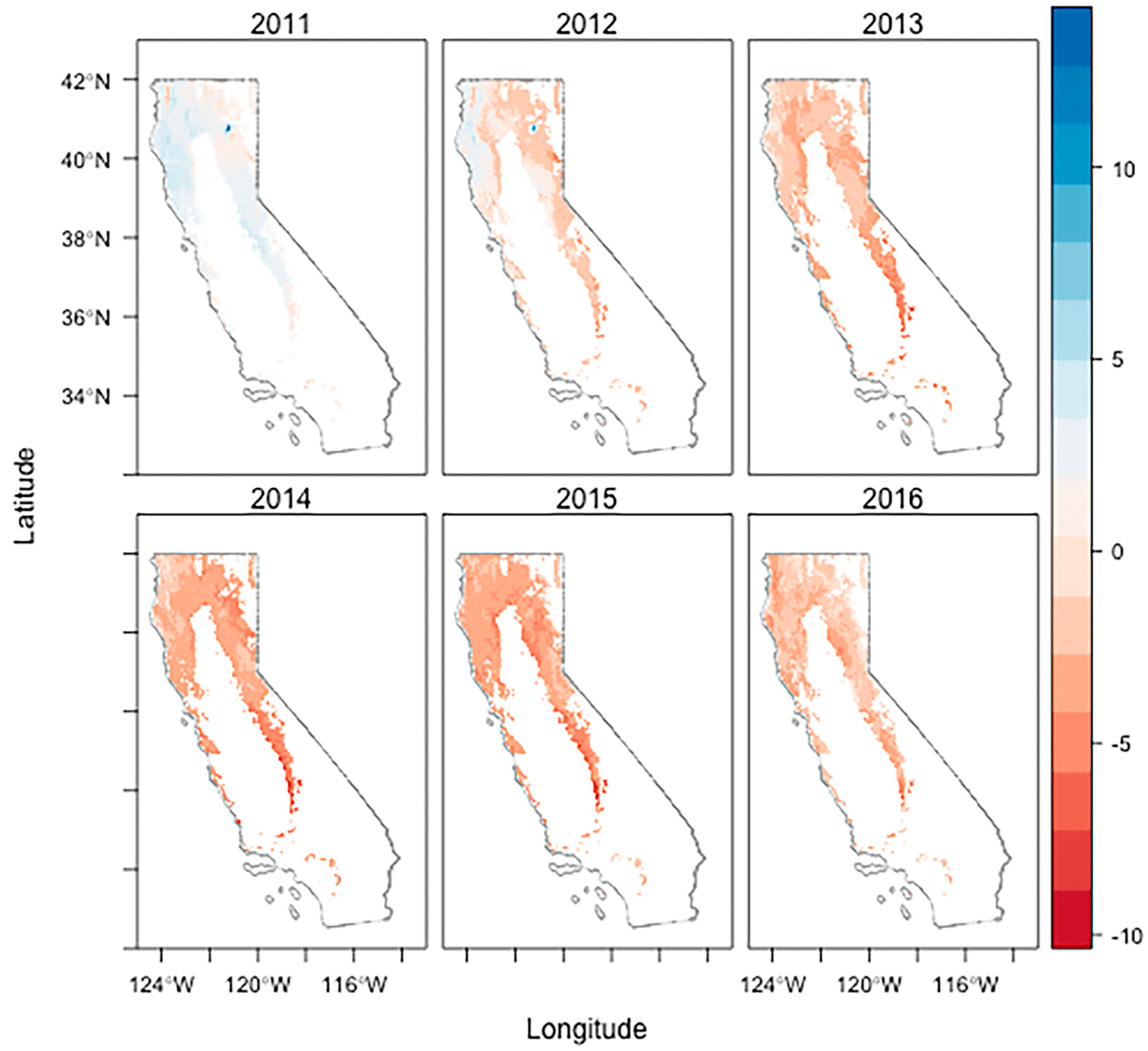
2.2. The Most Severe Drought on Record

In California, the 2012–2016 drought was the most severe on record. With forested areas representing 43% of the state’s natural area (Figure 1), multiple years of extended severe drought (Diffenbaugh et al., 2015; Figure 2) make California an important case study to evaluate the use of remote sensing products to understand large-scale patterns in tree mortality. The self-calibrated Palmer drought severity index (scPDSI; Table 1; Figure 2) was used to quantify drought severity and to calculate the frequency of severe drought (2002–2015). The scPDSI is an improved version of the Palmer Drought Severity Index, which has been widely used to monitor drought conditions [4,36,37,38,39,40,41,42,43]. Monthly scPDSI data was available through the Western Regional Climate Center (https://www.wrcc.dri.edu/). The scPDSI ranges from −10 to 10, with the number indicating the magnitude and the sign denoting (+) wetter than average or (−) drier than average conditions for a location based on historical climate and sensitivity to changes in water availability [38]. Values of scPDSI between −0.4 and 0.4 denote average conditions and absolute values greater than 3 are indicative of severe conditions. Severe conditions occur based on the history of the location and are not determined relative to a default location [38]. The scPDSI has a similar range of variability in diverse climates, allowing for more exact comparisons between locations and times [38,44]. The scPDSI has been widely used for drought characterization [44,45,46].

2.3. Ecosystem Water Use Efficiency
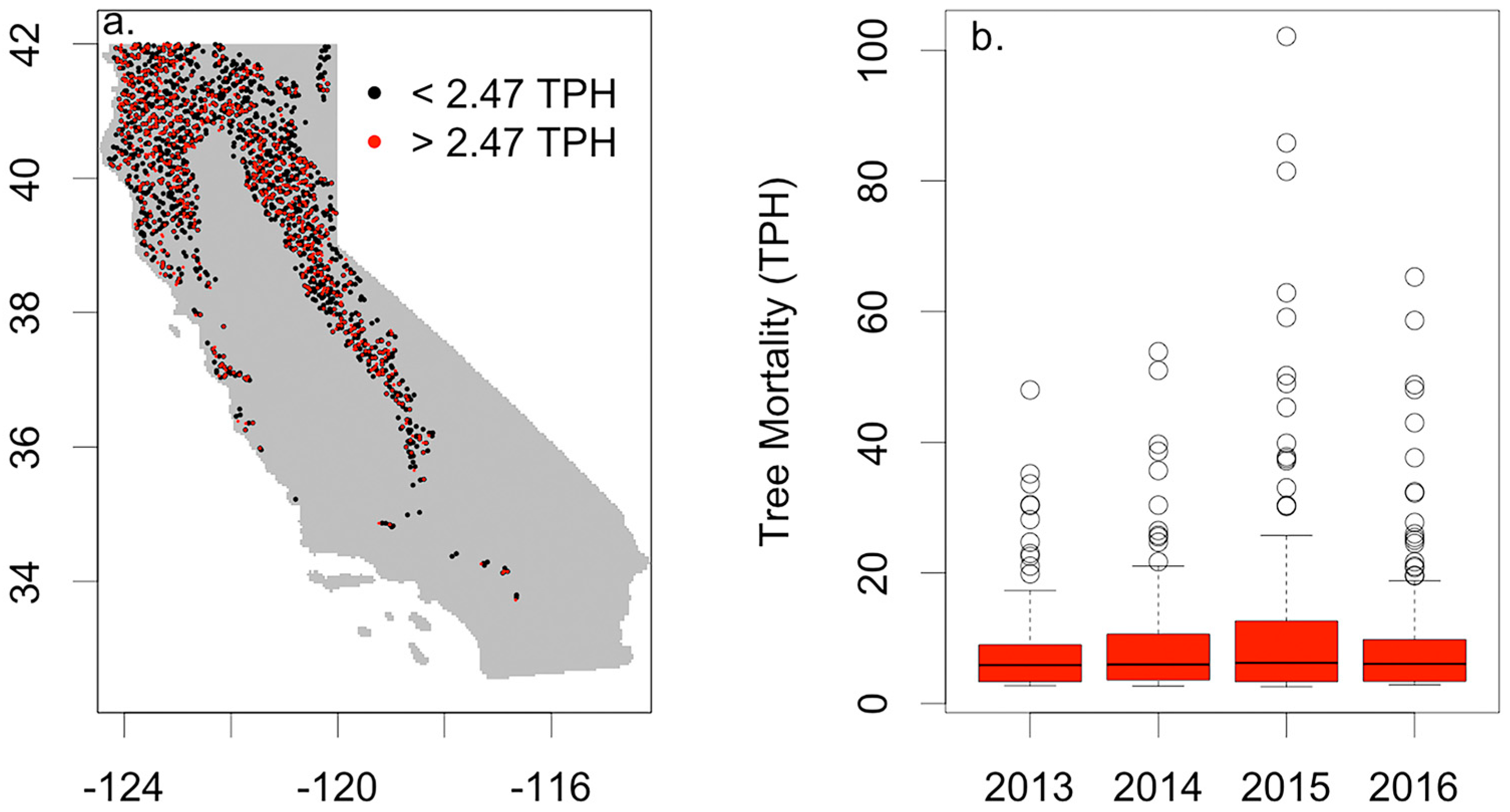
Water use efficiency is recognized as an important characteristic of productivity in various natural scientific disciplines and has been used recently at the ecosystem level [8,16,47,48,49,50,51]. Ecologists commonly use the ratio of ecosystem fluxes such as NPP [8,16,52], net ecosystem productivity/exchange (NEP/NEE) [49,50], or gross primary productivity (GPP) [48] to water loss (ET or transpiration; [19,48,53] as a measure of WUE.
We obtained MODIS GPP (MOD17) [54,55] and ET (MOD16) [56] data that were processed and made available by the Numerical Terradynamic Simulation Group at the University of Montana to calculate WUE [8] (Table 1). A comparison of annual WUE (2007–2014) derived from MODIS layers and WUE measured with the eddy covariance method at three tower sites in California forests showed that MODIS WUE captured temporal trends in WUE (R2 = 0.40; p < 0.001), although gross primary productivity (R2 = 0.78; p < 0.001) was overestimated and ET was underestimated (R2 = 0.90; p < 0.001) [8]. Differences between tower WUE and MODIS WUE were likely due to the limited sampling period in Eddy covariance data (2007 to 2014 for most tower sites). Additional limitations of this comparison are that tower sites represent just three forest types in the Sierra Nevada’s (oak pine forest, ponderosa pine forest, and Sierra mixed conifer forests), the sample size was small (n = 16), there were large differences in the sampling area for tower sites (hundreds of meters) and MODIS pixels (4 km), and comparisons occur mostly during drought years preventing an extensive evaluation of how tower based WUE varies overtime in comparison to MODIS WUE.
Deviations in WUE in 2014 (WUESevere Drought) from WUEBASELINE (i.e., ΔWUE) were used to explore patterns in maximum tree mortality rates (2013–2016) for all forested areas in California. We defined WUEBASELINE by extracting values of annual WUE under normal conditions (i.e., mean annual scPDSI between −0.04 and 0.04) from 2002–2013. Values were averaged across climate ecoregions (http://data.fs.usda.gov/geodata) to fill gaps in forested locations that were not under normal conditions from 2002–2013 [8]. The lag between 2014 ΔWUE and maximum tree mortality rates in 2015–2016 will aide our ability to capture drought induced mortality, which is often delayed [4].

2.4. Tree Mortality

The USDA Forest Service Forest Health and Monitoring (FHM) program conducts aerial detection surveys for California forest (USFS Region 5) annually and data is available from 1978 to the present (https://www.fs.usda.gov/detail/r5/forest-grasslandhealth/?cid=fsbdev3_046696). Surveys were done by flying over the forests and sketch mapping areas of mortality, recording the mortality agent, forest type, and affected trees per hectare (TPH). Mortality was detected by identifying yellow to reddish brown tree crowns. Areas identified by discolored tree crowns were categorized by (a) damage type (i.e., mortality, top kill, defoliation); (b) the number of trees affected (TPH); and (c) the affected tree species. Surveyors also recorded the probable damage-causing agent (i.e., fire, bark beetles, etc.). If the damage-causing agent was unknown at the time of the flight, the local Forest Service entomologist and/or pathologist determined the likely agent. Generally, areas with <2.47 TPH of mortality were considered to have “background” or “normal” levels of mortality and were not mapped. Although, if low levels of mortality were indicative of a localized pest-related event then areas were mapped. Annual mortality surveys were compiled (2013–2016) and the maximum TPH was used to develop a gridded mortality layer. This layer was designed to match the resolution of WUE layers (1 km; Table 1).
The maximum tree mortality layer is an estimate of maximum tree mortality rates within a 1 km pixel. While appropriate for examining large-scale patterns in tree mortality, it is useful to understand patterns in tree mortality that exist at finer scales. Forest Inventory and Analysis (FIA) data will be used to evaluate plot level patterns in tree mortality. We will compare annual FHP data to FIA plots (n = 1390) that were measured in 2013–2016. Although there are 6000 FIA plots in California, only a portion of plots are measured in a given year (~10%). Mortality rates observed on a plot level (TPH year−1.) are unlikely to reflect landscape mortality patterns recorded in the FHP survey. In areas where tree mortality was sketch mapped, plots are likely to have higher than background (>2.47 TPH) mortality rates.

2.5. Statistical Analysis

We used a regression tree approach to estimate maximum tree mortality rates (TPH) in California forests. Tree-based models are a supervised machine learning method commonly used in ecology for exploratory data analysis and prediction, due to their simplistic nonparametric design. This approach recursively partitions the data into increasingly homogenous groups based on values that minimize a loss function (i.e., Sum of Squared Errors (SSE) for regression). Tree-based models were developed in R [57] using the package rpart [58,59]. The rpart package creates a regression tree based on binary splits that maximize homogeneity and minimizes impurity. The output is a single decision tree that can be further “pruned” or trimmed back using the cross-validation error statistic to reduce over-fitting. Regression trees are ideally suited for the analysis of complex ecological data [60]. We used this approach to estimate maximum tree mortality rates [58,60,61], and included ΔWUE, WUEBASELINE, mean annual scPDSI in 2014 and 2015, and the frequency of severe drought (i.e., mean annual scPDSI < −3) from 2002–2015 in the model as explanatory parameters. We evaluated post drought maximum mortality rates using the FHP mortality data and used the FIA data to evaluate tree mortality patterns at the plot level. Data processing was carried out using the program R 3.3.2 [57] and the packages rgdal [62], and raster [63].

3. Results

In California, drought conditions began in 2012 after a brief wet period (Figure 2 and Figure 3). In 2013, all forested areas were under severe drought. The majority of the state, ~80%, was in extreme to extraordinary drought in 2014 and ~100% was in severe drought or worse. These conditions were maintained throughout 2016, making the 2012–2016 drought the longest, most severe drought on record. The frequency of severe drought (2002–2016) ranged from 1 to 11 years with a mean of four years. The majority of forested area (52%) had a severe drought frequency that was ≥3 years.

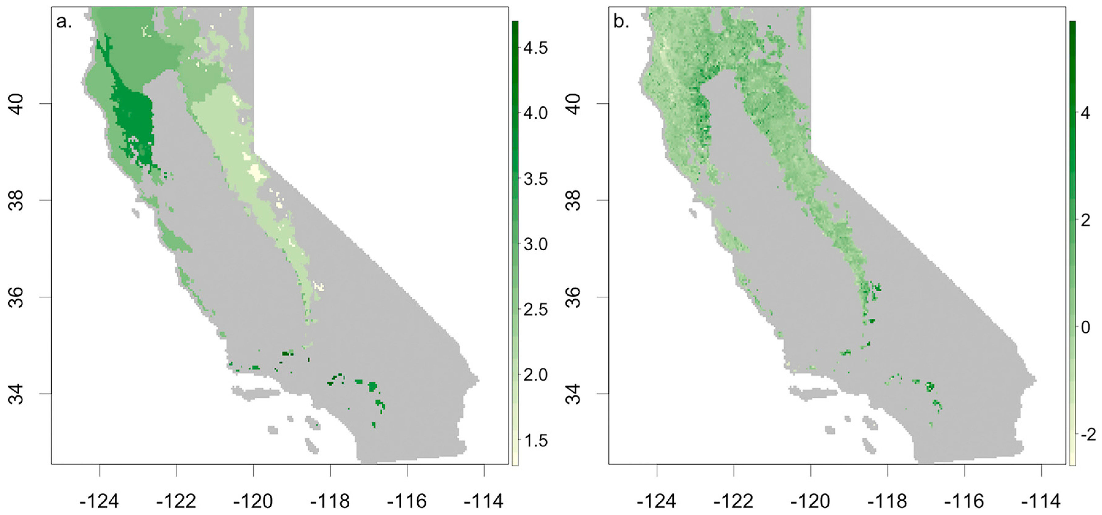
3.1. Ecosystem Water Use Efficiency

Determined under normal, non-drought conditions, WUEBASELINE varied across California forests and ecoregions (Figure 4a). Ranging between 1.3 to 4.7 g C/mm H2O, WUEBASELINE was generally higher in arid regions. The highest WUEBASELINE occurred in the southern portion of the state, in the California Mountain Valley and to the north in the Northern California Range (>2 g C/mm H2O). The lowest WUEBASELINE occurred in the eastern half of the state in the Modoc Plateau and the Sierra Nevada’s. WUE declined in many areas under drought conditions, compared to WUEBASELINE, and in 2014 ΔWUE ranged between −2.6 and 5.7 (g C/mm H2O; Figure 4b). While resilient ecosystems maintained or increased (70% of forested land) in WUE under severe drought conditions, 30% of forested area had a ΔWUE that was less than 0.

3.2. Drought Induced Tree Mortality

Patterns in plot level data indicate that mortality was patchy and peaked in 2015 (Figure 5). In 2013, 38% of FIA plots measured in forested areas (n = 334 plots) exhibited elevated tree mortality rates (TPH > 2.47) and by 2016 elevated mortality increased to 44% of FIA plots measured (n = 331). Just 104 FIA plots overlapped with FHP mapped mortality from 2013–2016. Just less than half (46%) of those plots exhibited elevated mortality rates. The mean tree mortality rate in FIA plots with elevated tree mortality was similar across drought years (Figure 5b), although the maximum TPH was 48 TPH in 2013, which increased to 102 TPH in 2015 and 65 TPH in 2016.
In 2011, prior to the onset of drought (2012), 1.7 million dead trees (1.3 million ha) were detected in areas where bark beetles were active (FHP mortality survey). Between 2002 and 2016, the majority of forested land (63%) was under severe drought conditions for more than 3 years. Trees killed increased in 2014 to 2.9 million trees and escalated substantially in 2015 to 26 million trees. FIA plots suggest that tree mortality rates peaked in 2015, which is the year with the greatest increase in impacted area mapped by FHP. By 2016, 59 million trees were killed and the majority of these trees (82%; 8 million ha) were in areas with active bark beetles. Maximum tree mortality rates ranged from 0 to 300 TPH, with the highest rates occurring in the Sierra Nevada’s (Figure 6).

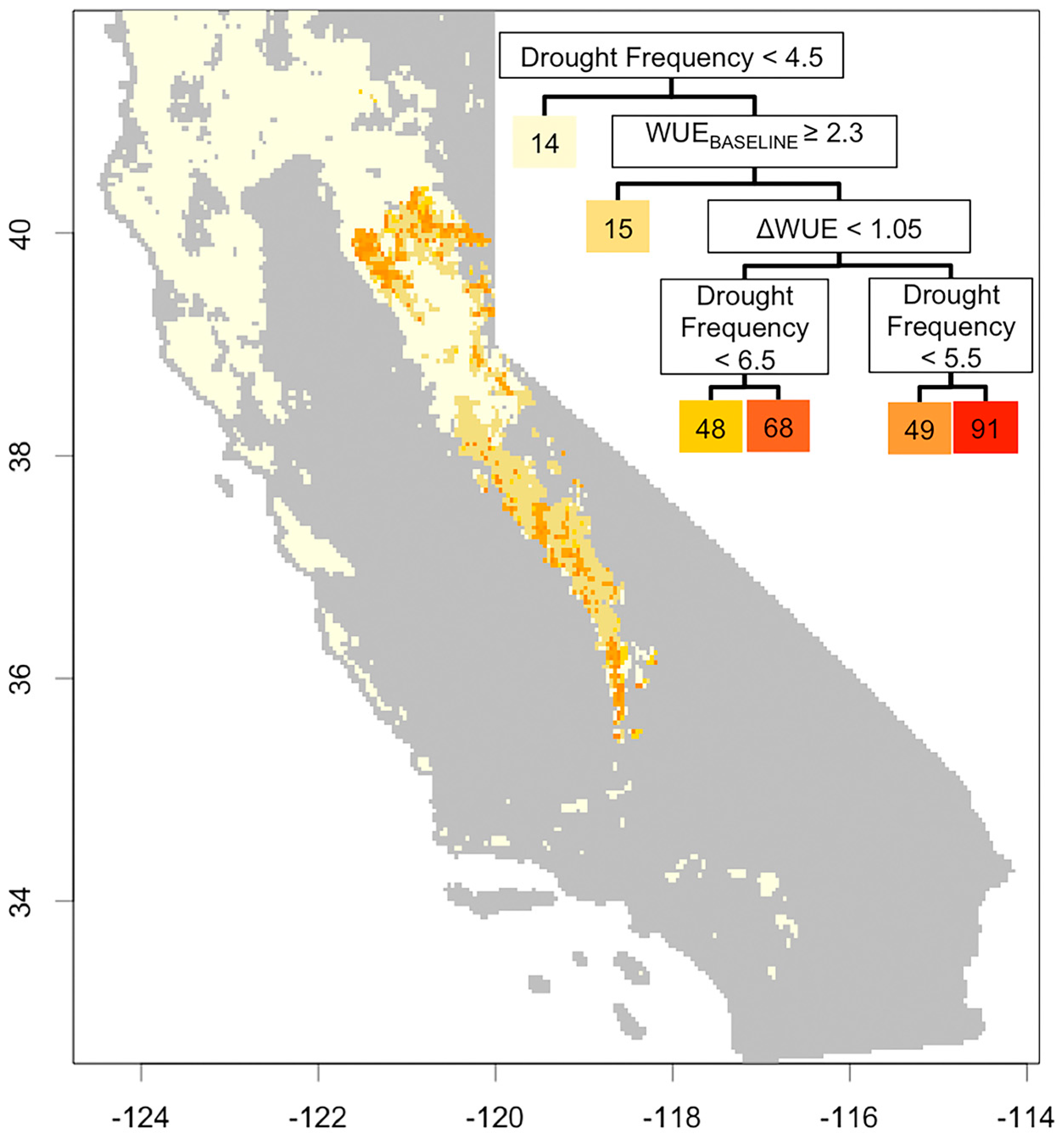
3.3. Understanding Drought Induced Tree Mortality

Drought frequency, WUEBASELINE, and ΔWUE were important for explaining drought induced maximum tree mortality rates at the ecosystem scale (Figure 7). Tree mortality was classified into six classes: 14, 15, 48, 49, 68, and 91 TPH. The majority of forested area had an estimated mortality rate of 14 TPH (63%), and just 2% of all forested land had mortality rates as high as 91 TPH. California forest with a drought frequency <4.5 years had the lowest average tree mortality (14 TPH). Where drought frequency was >4.5 years, WUEBASELINE was important for understanding the level of enhanced drought induced mortality rates. Even under high severe drought frequencies (>4.5 years), a WUEBASELINE ≥2.35 g C/mm H2O was associated with a very small increase in tree mortality rates (15 TPH). Where WUEBASELINE was <2.35 g C/mm H2O, dramatic increases in tree mortality co-occurred with the interaction of ΔWUE and the frequency of severe drought. Surprisingly, lower values of ΔWUE were associated with lower tree mortality rates when severe drought frequency was high. Variable importance, the reduction in mean squared error attributed to each variable, was greatest for drought frequency (0.28), followed by WUEBASELINE (0.21), and ΔWUE (0.1). Together, drought frequency, WUEBASELINE, and ΔWUE accounted for 23% of the variation in drought induced tree mortality rates.

4. Discussion

A critical link between carbon and water cycles in terrestrial ecosystems, WUE is an effective way of assessing ecosystem response to drought [8,13,48,50,64,65]. Our results show that drought frequency, WUEBASELINE, and ΔWUE captured variation in post drought maximum tree mortality rates in California forests. As hypothesized, forested areas with lower WUEBASELINE were the most vulnerable to high post drought tree mortality. Surprisingly, the effects of ΔWUE varied and were dependent on severe drought frequency. Previous research suggested that a lower ΔWUE was indicative of a decline in ecosystem resilience under drought conditions [8]. While this may be true, in forested ecosystems a ΔWUE > 0 was associated with the highest tree mortality rates when drought frequencies where high. Combined with high drought frequencies (>5 years) in recent years, substantial increases in drought induced tree mortality were detected in areas where bark beetles were active. Here, changes in WUE were in response to extreme prolonged drought and were important for understanding patterns in forest dieback.
Mortality rates have been increasing since 1983 in California forests [66]. This increase in mortality is thought to be a response to the gradual temperature-driven rise in water stress, pests and pathogens [66]. The steady gradual increase in mortality has been concentrated in small trees [66] and until the most recent drought (2012–2015), climate conditions remained below thresholds that could cause large-scale forest die-back. In the 2012–2016 drought, the cumulative rainfall deficit was described as a one in a 1000-year event [37], and resulted in severely reduced snowpack, soil moisture, groundwater, and reservoir stocks [5]. This increase in water deficit, combined with high air temperatures and insect infestations, generated a large pulse of tree mortality in California [5]. Unlike the gradual increase in tree mortality since 1983, the 2012–2016 drought led to mortality in large trees [5]. Approximately 10.6 million ha of forest containing up to 888 million large trees experienced measurable loss in canopy water content [5]. Severe canopy water losses of greater than 30% occurred over 1 million ha, affecting up to 58 million large trees [5].
Drought affects virtually every plant process and the magnitude of the effect depends on drought severity and duration as well as the plant’s developmental stage [28,67]. One of the most sensitive and immediate responses to water stress at the cellular level is a reduction in growth processes (i.e., cell division and enlargement) [67]. Photosynthesis itself declines only slowly until water stress becomes moderate to severe [67,68]. Monitoring changes in WUE allows us to track changes in photosynthesis by monitoring shifts in greenness and measuring how greenness scales with water availability. Although photosynthesis declines with drought conditions, carbon uptake per mm of ET often becomes more efficient, resulting in an increase in WUE. Our results indicate that a low WUEBASELINE at the ecosystem scale was linked to enhance mortality rates and that the interaction of the frequency of severe drought and ΔWUE were important for understanding high rates of drought induced tree mortality.
Substantial evidence indicates that drought stress promotes insect outbreaks, which are typically preceded by unusually warm, dry weather [28]. Drought provides a more favorable thermal environment for insect growth and because insects have limited thermoregulatory capacities, the higher air and host plant temperatures associated with drought enable them to grow and reproduce in a more optimal temperature regime. Optimal temperature regimes, without changes in food quality, will permit insects to grow faster and larger, suffer less mortality, and lay more eggs per unit of ingested food [28]. Leaf yellowing, higher temperatures, and greater infrared reflectance of drought-stressed plants may make them more attractive or acceptable to insects [28] and some plants become more susceptible to certain insects during severe drought owing strictly to a decline in defenses [28]. Our results suggest that spatial and temporal patterns in WUEBASELINE and ΔWUE detected in areas with high mortality rates are a reflection of both climate-induced physiological stress (declines in photosynthesis under severe drought) and interactions with other climate-mediated processes (i.e., bark beetle outbreaks).

5. Conclusions

Water-limited forests are sensitive to temperature-driven drought stress, and may be poised for dieback if future climates continue to feature rising temperatures without compensating increases in precipitation [66]. Climate change is expected to increase average temperatures in California by about 2.4 °C in the next 100 years, but the prevailing precipitation regime is not expected to change [69,70,71]. Our findings strongly suggest that if severe drought becomes more frequent, we can expect regional scale forest change [5]. An increase in the frequency of severe drought has the potential to cause rapid vegetation change through drought-induced forest dieback as different species replace contemporary forest dominants [4], and may have cascading effects on forest fire susceptibility and severity, animal habitat, biological diversity, water resources, and carbon sequestration. Monitoring changes in WUE captures ecosystem scale response to drought and can be used to understand drought vulnerability and how it changes over time with climate conditions.

Acknowledgments

The author would like to acknowledge the excellent support provided Rocky Mountain Research Station (RMRS) and Florida International University (FIU). This research builds on research [8] that was initiated at the Open Science for Synthesis-2014 training (supported by the National Science Foundation under Grant No. OCI-1216894) at the National Center for Ecological Analysis and Synthesis (NCEAS), a center funded by the University of California, Santa Barbara, and the State of California. The authors would also like to thank the Goulden Lab at the University of California Irvine. Any opinions, findings, conclusions or recommendations expressed in this material are those of the author and do not necessarily reflect the views of RMRS, FIU, or NCEAS.

Conflicts of Interest

The authors declare no conflict of interest.

References

  1. Allen, C.D.; Breshears, D.D. Drought-induced shift of a forest–woodland ecotone: Rapid landscape response to climate variation. Proc. Natl. Acad. Sci. USA 1998, 95, 14839–14842. [Google Scholar] [CrossRef] [PubMed]
  2. Allen, C.D.; Macalady, A.K.; Chenchouni, H.; Bachelet, D.; McDowell, N.; Vennetier, M.; Kitzberger, T.; Rigling, A.; Breshears, D.D.; Hogg, E.H.; et al. A global overview of drought and heat-induced tree mortality reveals emerging climate change risks for forests. For. Ecol. Manag. 2010, 259, 660–684. [Google Scholar] [CrossRef]
  3. Boisvert-Marsh, L.; Perie, C.; de Blois, S. Shifting with climate? Evidence for recent changes in tree species distribution at high latitudes. Ecosphere 2014, 5, 1–33. [Google Scholar] [CrossRef]
  4. Guarín, A.; Taylor, A.H. Drought triggered tree mortality in mixed conifer forests in Yosemite National Park, California, USA. For. Ecol. Manag. 2005, 218, 229–244. [Google Scholar] [CrossRef]
  5. Asner, G.P.; Brodrick, P.G.; Anderson, C.B.; Vaughn, N.; Knapp, D.E.; Martin, R.E. Progressive forest canopy water loss during the 2012–2015 California drought. Proc. Natl. Acad. Sci. USA 2016, 113, E249–E255. [Google Scholar] [CrossRef] [PubMed]
  6. Diffenbaugh, N.S.; Pal, J.S.; Trapp, R.J.; Giorgi, F. Fine-scale processes regulate the response of extreme events to global climate change. Proc. Natl. Acad. Sci. USA 2005, 102, 15774–15778. [Google Scholar] [CrossRef] [PubMed]
  7. Bonan, G.B. Forests and climate change: Forcings, feedbacks, and the climate benefits of forests. Science 2008, 320, 1444–1449. [Google Scholar] [CrossRef] [PubMed]
  8. Malone, S.L.; Tulbure, M.G.; Pérez-Luque, A.J.; Assal, T.J.; Bremer, L.L.; Drucker, D.P.; Hillis, V.; Varela, S.; Goulden, M.L. Drought resistance across California ecosystems: Evaluating changes in carbon dynamics using satellite imagery. Ecosphere 2016. [Google Scholar] [CrossRef]
  9. Emmerich, W.E. Ecosystem Water Use Efficiency in a Semiarid Shrubland and Grassland Community. Rangel. Ecol. Manag. 2007, 60, 464–470. [Google Scholar] [CrossRef]
  10. Angeler, D.G.; Allen, C.R. Quantifying resilience. J. Appl. Ecol. 2016, 53, 617–624. [Google Scholar] [CrossRef]
  11. Huxman, T.E.; Smith, M.D.; Fay, P.A.; Knapp, A.K.; Shaw, M.R.; Loik, M.E.; Smith, S.D.; Tissue, D.T.; Zak, J.C.; Weltzin, J.F.; et al. Convergence across biomes to a common rain-use efficiency. Nature 2004, 429, 651–654. [Google Scholar] [CrossRef] [PubMed]
  12. Reichstein, M.; Ciais, P.; Papale, D.; Valentini, R.; Running, S.; Viovy, N.; Cramer, W.; Granier, A.; Ogée, J.; Allard, V.; et al. Reduction of ecosystem productivity and respiration during the European summer 2003 climate anomaly: A joint flux tower, remote sensing and modelling analysis. Glob. Chang. Biol. 2007, 13, 634–651. [Google Scholar] [CrossRef]
  13. Bai, Y.; Wu, J.; Xing, Q.; Pan, Q.; Huang, J.; Yang, D.; Han, X. Primary production and rain use efficiency across a precipitation gradient on the Mongolia Plateau. Ecology 2008, 89, 2140–2153. [Google Scholar] [CrossRef] [PubMed]
  14. Lu, X.; Zhuang, Q. Evaluating evapotranspiration and water-use efficiency of terrestrial ecosystems in the conterminous United States using MODIS and AmeriFlux data. Remote Sens. Environ. 2010, 114, 1924–1939. [Google Scholar] [CrossRef]
  15. Zhu, Q.; Jiang, H.; Peng, C.; Liu, J.; Wei, X.; Fang, X.; Liu, S.; Zhou, G.; Yu, S. Evaluating the effects of future climate change and elevated CO2 on the water use efficiency in terrestrial ecosystems of China. Ecol. Model. 2011, 222, 2414–2429. [Google Scholar] [CrossRef]
  16. Liu, Y.; Xiao, J.; Ju, W.; Zhou, Y.; Wang, S.; Wu, X. Water use efficiency of China’s terrestrial ecosystems and responses to drought. Sci. Rep. 2015, 5, 13799. [Google Scholar] [CrossRef] [PubMed]
  17. Yang, Y.; Guan, H.; Batelaan, O.; McVicar, T.R.; Long, D.; Piao, S.; Liang, W.; Liu, B.; Jin, Z.; Simmons, C.T. Contrasting responses of water use efficiency to drought across global terrestrial ecosystems. Sci. Rep. 2016, 6, 23284. [Google Scholar] [CrossRef] [PubMed]
  18. Ponce Campos, G.E.; Moran, M.S.; Huete, A.; Zhang, Y.; Bresloff, C.; Huxman, T.E.; Eamus, D.; Bosch, D.D.; Buda, A.R.; Gunter, S.A.; et al. Ecosystem resilience despite large-scale altered hydroclimatic conditions. Nature 2013, 494, 349–352. [Google Scholar] [CrossRef] [PubMed]
  19. Reichstein, M.; Tenhunen, J.D.; Roupsard, O.; Ourcival, J.-M.; Rambal, S.; Miglietta, F.; Peressotti, A.; Pecchiari, M.; Tirone, G.; Valentini, R. Severe drought effects on ecosystem CO2 and H2O fluxes at three Mediterranean evergreen sites: Revision of current hypotheses? Glob. Chang. Biol. 2002, 8, 999–1017. [Google Scholar] [CrossRef]
  20. Villalba, R.; Veblen, T.T. Influence of Large-scale Climatic Variability on Episodic Tree Mortality in Northern Patagonia. Ecology 1998, 79, 2624–2640. [Google Scholar] [CrossRef]
  21. Fensham, R.J.; Holman, J.E. Temporal and spatial patterns in drought-related tree dieback in Australian savanna. J. Appl. Ecol. 1999, 36, 1035–1050. [Google Scholar] [CrossRef]
  22. Williamson, G.B.; Laurance, W.F.; Oliveira, A.A.; Delamonica, P.; Gascon, C.; Lovejoy, T.E.; Pohl, L. Amazonian tree mortality during the 1997 El Nino drought. Conserv. Biol. 2000, 14, 1538–1542. [Google Scholar] [CrossRef]
  23. Ferrell, G.T.; Otrosina, W.J.; Demars, C.J., Jr. Predicting susceptibility of white fir during a drought-associated outbreak of the fir engraver, Scolytus ventralis, in California. Can. J. For. Res. 1994, 24, 302–305. [Google Scholar] [CrossRef]
  24. Speer, J.H.; Swetnam, T.W.; Wickman, B.E.; Youngblood, A. Changes in pandora moth outbreak dynamics during the past 622 Years. Ecology 2001, 82, 679–697. [Google Scholar] [CrossRef]
  25. Macomber, S.A.; Woodcock, C.E. Mapping and monitoring conifer mortality using remote sensing in the Lake Tahoe Basin. Remote Sens. Environ. 1994, 50, 255–266. [Google Scholar] [CrossRef]
  26. Savage, M. Anthropogenic and natural disturbance and patterns of mortality in a mixed conifer forest in California. Can. J. For. Res. 1994, 24, 1149–1159. [Google Scholar] [CrossRef]
  27. Savage, M. The role of anthropogenic influences in a mixed-conifer forest mortality episode. J. Veg. Sci. 1997, 8, 95–104. [Google Scholar] [CrossRef]
  28. Mattson, W.J.; Haack, R.A. The Role of Drought in Outbreaks of Plant-Eating Insects. Bioscience 1987, 37, 110–118. [Google Scholar] [CrossRef]
  29. Kobe, R.K.; Pacala, S.W.; Silander, J.A.; Canham, C.D. Juvenile Tree Survivorship as a Component of Shade Tolerance. Ecol. Appl. 1995, 5, 517–532. [Google Scholar] [CrossRef]
  30. Pacala, S.W.; Canham, C.D.; Saponara, J.; Silander, J.A.; Kobe, R.K.; Ribbens, E. Forest Models Defined by Field Measurements: Estimation, Error Analysis and Dynamics. Ecol. Monogr. 1996, 66, 1–43. [Google Scholar] [CrossRef]
  31. Wyckoff, P.H.; Clark, J.S. The relationship between growth and mortality for seven co-occurring tree species in the southern Appalachian Mountains. J. Ecol. 2002, 90, 604–615. [Google Scholar] [CrossRef]
  32. Intergovernmental Panel on Climate Change (IPCC). The Physical Science Basis. Contribution of Working Group I to the Fifth Assessment Report of the Intergovernmental Panel on Climate Change; Cambridge University Press: Cambridge, UK; New York, NY, USA, 2013. [Google Scholar]
  33. Bailey, R.G. Description of the Ecoregions of the United States; No. 1391; USDA Forest Service: Ogden, Utah, 1995.
  34. Christensen, G.A.; Waddell, K.L.; Stanton, S.M.; Kuegler, O. California’s Forest Resources: Forest Inventory and Analysis, 2001–2010; U.S. Forest Service: Portland, Oregon, 2016.
  35. Friedl, M.A.; Sulla-Menashe, D.; Tan, B.; Schneider, A.; Ramankutty, N.; Sibley, A.; Huang, X. MODIS Collection 5 global land cover: Algorithm refinements and characterization of new datasets. Remote Sens. Environ. 2010, 114, 168–182. [Google Scholar] [CrossRef]
  36. Piechota, T.C.; Dracup, J.A. Drought and Regional Hydrologic Variation in the United States: Associations with the El Niño-Southern Oscillation. Water Resour. Res. 1996, 32, 1359–1373. [Google Scholar] [CrossRef]
  37. Robeson, S.M. Revisiting the recent California drought as an extreme value. Geophys. Res. Lett. 2015, 42, 2015GL064593. [Google Scholar] [CrossRef]
  38. Wells, N.; Goddard, S.; Hayes, M.J. A Self-Calibrating Palmer Drought Severity Index. J. Clim. 2004, 17, 2335–2351. [Google Scholar] [CrossRef]
  39. Hessburg, P.F.; Kuhlmann, E.E.; Swetnam, T.W. Examining the Recent Climate through the Lens of Ecology: Inferences from Temporal Pattern Analysis. Ecol. Appl. 2005, 15, 440–457. [Google Scholar] [CrossRef]
  40. Klos, R.J.; Wang, G.G.; Bauerle, W.L.; Rieck, J.R. Drought impact on forest growth and mortality in the southeast USA: An analysis using Forest Health and Monitoring data. Ecol. Appl. 2009, 19, 699–708. [Google Scholar] [CrossRef] [PubMed]
  41. Littell, J.S.; McKenzie, D.; Peterson, D.L.; Westerling, A.L. Climate and wildfire area burned in western U.S. ecoprovinces, 1916–2003. Ecol. Appl. 2009, 19, 1003–1021. [Google Scholar] [CrossRef] [PubMed]
  42. Hart, S.J.; Veblen, T.T.; Eisenhart, K.S.; Jarvis, D.; Kulakowski, D. Drought induces spruce beetle (Dendroctonus rufipennis) outbreaks across northwestern Colorado. Ecology 2014, 95, 930–939. [Google Scholar] [CrossRef] [PubMed]
  43. Zhang, B.; Zhang, L.; Guo, H.; Leinenkugel, P.; Zhou, Y.; Li, L.; Shen, Q. Drought impact on vegetation productivity in the Lower Mekong Basin. Int. J. Remote Sens. 2014, 35, 2835–2856. [Google Scholar] [CrossRef]
  44. Schrier, G.; Barichivich, J.; Briffa, K.R.; Jones, P.D. A scPDSI-based global data set of dry and wet spells for 1901–2009. J. Geophys. Res. D Atmos. 2013, 118, 4025–4048. [Google Scholar] [CrossRef]
  45. Busby, S.J. Simulating multiyear drought events in North America with the HadCM3 climate model. Weather 2008, 63, 240–243. [Google Scholar] [CrossRef]
  46. Yu, M.; Liu, X.; Wei, L.; Li, Q.; Zhang, J.; Wang, G. Drought Assessment by a Short-/Long-Term Composited Drought Index in the Upper Huaihe River Basin, China. Adv. Meteorol. 2015, 2016. [Google Scholar] [CrossRef]
  47. Hu, Z.; Yu, G.; Fu, Y.; Sun, X.; Li, Y.; Shi, P.; Wang, Y.; Zheng, Z. Effects of vegetation control on ecosystem water use efficiency within and among four grassland ecosystems in China. Glob. Chang. Biol. 2008, 14, 1609–1619. [Google Scholar] [CrossRef]
  48. Kuglitsch, F.G.; Reichstein, M.; Beer, C.; Carrara, A.; Ceulemans, R.; Granier, A.; Janssens, I.A.; Koestner, B.; Lindroth, A.; Loustau, D.; et al. Characterisation of ecosystem water-use efficiency of european forests from eddy covariance measurements. Biogeosci. Discuss 2008, 5, 4481–4519. [Google Scholar] [CrossRef]
  49. Monson, R.K.; Prater, M.R.; Hu, J.; Burns, S.P.; Sparks, J.P.; Sparks, K.L.; Scott-Denton, L.E. Tree species effects on ecosystem water-use efficiency in a high-elevation, subalpine forest. Oecologia 2010, 162, 491–504. [Google Scholar] [CrossRef] [PubMed]
  50. Niu, S.; Xing, X.; Zhang, Z.; Xia, J.; Zhou, X.; Song, B.; Li, L.; Wan, S. Water-use efficiency in response to climate change: From leaf to ecosystem in a temperate steppe. Glob. Chang. Biol. 2011, 17, 1073–1082. [Google Scholar] [CrossRef]
  51. Tang, X.; Li, H.; Desai, A.R.; Nagy, Z.; Luo, J.; Kolb, T.E.; Olioso, A.; Xu, X.; Yao, L.; Kutsch, W.; et al. How is water-use efficiency of terrestrial ecosystems distributed and changing on Earth? Sci. Rep. 2014, 4, 7483. [Google Scholar] [CrossRef] [PubMed] [Green Version]
  52. Roupsard, O.; le Maire, G.; Nouvellon, Y.; Dauzat, J.; Jourdan, C.; Navarro, M.; Bonnefond, J.-M.; Saint-André, L.; Mialet-Serra, I.; Hamel, O.; et al. Scaling-up productivity (NPP) using light or water use efficiencies (LUE, WUE) from a two-layer tropical plantation. Agrofor. Syst. 2009, 76, 409–422. [Google Scholar] [CrossRef]
  53. Law, B.E.; Falge, E.; Gu, L.; Baldocchi, D.D.; Bakwin, P.; Berbigier, P.; Davis, K.; Dolman, A.J.; Falk, M.; Fuentes, J.D.; et al. Environmental controls over carbon dioxide and water vapor exchange of terrestrial vegetation. Agric. For. Meteorol. 2002, 113, 97–120. [Google Scholar] [CrossRef]
  54. Zhao, M.; Heinsch, F.A.; Nemani, R.R.; Running, S.W. Improvements of the MODIS terrestrial gross and net primary production global data set. Remote Sens. Environ. 2005, 95, 164–176. [Google Scholar] [CrossRef]
  55. Running, S.W.; Zhao, M. Daily GPP and Annual NPP (MOD17A2/A3) Products NASA Earth Observing System MODIS Land Algorithm; Numerical Terradynamic Simulation Group: Missoula, MT, USA, 2015. [Google Scholar]
  56. Mu, Q.; Heinsch, F.A.; Zhao, M.; Running, S.W. Development of a global evapotranspiration algorithm based on MODIS and global meteorology data. Remote Sens. Environ. 2007, 111, 519–536. [Google Scholar] [CrossRef]
  57. R Development Core Team. R: A Language and Environment for Statistical Computing; R Foundation for Statistical Computing: Vienna, Austria, 2016. [Google Scholar]
  58. Loh, W.-Y. Classification and Regression Tree Methods. In Encyclopedia of Statistics in Quality and Reliability; John Wiley & Sons, Ltd.: Hoboken, New Jersey, 2008; ISBN 9780470061572. [Google Scholar]
  59. Therneau, T.; Atkinson, B.; Ripley, B. Rpart: Recursive Partitioning and Regression Trees. Available online: cran.r-project.org (accessed on 3 August 2017).
  60. De’ath, G.; Fabricius, K.E. Classification and Regression Trees: A Powerful Yet Simple Technique for Ecological Data Analysis. Ecology 2000, 81, 3178–3192. [Google Scholar] [CrossRef]
  61. Prasad, A.M.; Iverson, L.R.; Liaw, A. Newer Classification and Regression Tree Techniques: Bagging and Random Forests for Ecological Prediction. Ecosystems 2006, 9, 181–199. [Google Scholar] [CrossRef]
  62. Bivand, R.; Keitt, T.; Rowlingson, B.; Pebesma, E.; Sumner, M.; Hijmans, R.; Rouault, E. Rgdal: Bindings for the Geospatial Data Abstraction Library. Available online: cran.r-project.org (accessed on 3 August 2017).
  63. Hijmans, R.J.; van Etten, J.; Cheng, J.; Mattiuzzi, M.; Sumner, M.; Greenberg, J.A.; Lamigueiro, P.O.; Bevan, A.; Racine, E.B.; Shortridge, A. Raster: Geographic Data Analysis and Modeling. Available online: cran.r-project.org (accessed on 3 August 2017).
  64. Baldocchi, D. A comparative study of mass and energy exchange rates over a closed C3 (wheat) and an open C4 (corn) crop: II. CO2 exchange and water use efficiency. Agric. For. Meteorol. 1994, 67, 291–321. [Google Scholar] [CrossRef]
  65. Beer, C.; Ciais, P.; Reichstein, M.; Baldocchi, D.; Law, B.E.; Papale, D.; Soussana, J.-F.; Ammann, C.; Buchmann, N.; Frank, D.; et al. Temporal and among-site variability of inherent water use efficiency at the ecosystem level. Glob. Biogeochem. Cycles 2009, 23, GB2018. [Google Scholar] [CrossRef]
  66. Van Mantgem, P.J.; Stephenson, N.L. Apparent climatically induced increase of tree mortality rates in a temperate forest. Ecol. Lett. 2007, 10, 909–916. [Google Scholar] [CrossRef] [PubMed]
  67. Kramer, P.J. Water Relations of Plants; Academic Press: Orlando, FL, USA, 1983. [Google Scholar]
  68. Sharpe, P.J.H.; Wu, H.I.; Cates, R.G.; Coeschl, J.D. Energetics of Pine Defense Systems to Bark Beetle Attack; Forest Service General Technical Report SO.S6—United States; Southern Forest Experiment Station (USA): Beltsville, MD, USA; Washington, DC, USA, 1985.
  69. Leung, L.R.; Ghan, S.J. Pacific Northwest climate sensitivity simulated by a regional climate model driven by a GCM. Part II: 2 × CO2 simulations. J. Clim. 1999, 12, 2031–2053. [Google Scholar] [CrossRef]
  70. Dettinger, M.D.; Cayan, D.R.; Meyer, M.K.; Jeton, A.E. Simulated Hydrologic Responses to Climate Variations and Change in the Merced, Carson, and American River Basins, Sierra Nevada, California, 1900–2099. Clim. Chang. 2004, 62, 283–317. [Google Scholar] [CrossRef]
  71. Cayan, D.R.; Maurer, E.P.; Dettinger, M.D.; Tyree, M.; Hayhoe, K. Climate change scenarios for the California region. Clim. Chang. 2008, 87, 21–42. [Google Scholar] [CrossRef]
Figure 1. California’s distinct combinations of climate, elevation, and soil types create a unique mix of ecoregions and forest types. Forested areas are shown in grey and white areas represent non-forested land cover that was not included as part of this study. MODIS land cover type (MCD12Q1) in 2012 was used to identify forested areas [35]. The climate ecoregion layer was produced by the Forest Service Ecological Information and Mapping (ECOMAP) Team (https://data.fs.usda.gov/geodata).
Forests 08 00365 g001
Figure 2. Mean monthly scPDSI for all forested areas within California by latitude. The 2012–2016 drought was the most severe on record in terms of drought severity and duration.
Forests 08 00365 g002
Figure 3. Spatial and temporal patterns in mean annual scPDSI for forested areas in California. Drought condition began in 2012 and intensified and persisted throughout 2016.
Forests 08 00365 g003
Figure 4. Variation in (a) WUEBASELINE and (b) ΔWUE across California forests. Similar to patterns observed across California ecosystems [8], WUEBASELINE was highest in arid regions and ΔWUE in 2014 indicated that some areas exhibited resilience while others showed a decline in WUE from the baseline under extreme drought conditions. The latitude and longitude are shown along the axes.
Forests 08 00365 g004
Figure 5. (a) Forest Inventory Analysis (FIA) plots with elevated tree mortality rates (red) denote the patchy nature of mortality within forested areas. (b) Maximum post drought tree mortality in elevated FIA plots peaked in 2015. Latitude and longitude are shown along the axes.
Forests 08 00365 g005
Figure 6. Maximum tree mortality rates (2013–2016) (trees per hectare; TPH). Mortality data was derived from aerial detection surveys of California forest (USFS Region 5) 2013–2016 (http://egis.fire.ca.gov/TreeMortalityViewer/Help.html). Latitude and longitude are shown along the axes.
Forests 08 00365 g006
Figure 7. Estimates of maximum tree mortality (TPH) across California forests. The regression tree model of tree mortality showed that areas with high drought frequencies (years) and a low WUEBASELINE (<2.3 g C/mm H2O) exhibited elevated tree mortality rates. Where WUEBASELINE was <2.3 g C/mm H2O drought frequency and ΔWUE (g C/mm H2O) were essential in understanding changes in tree mortality rates. Latitude and longitude are shown along the axes.
Forests 08 00365 g007
Table 1. Federally funded datasets were used to evaluate patterns in tree mortality across California forests. Data was obtained from the National Aeronautics and Space Administration (NASA), the United States Department of Agriculture (USDA), and the United States Forest Service (USFS).
VariablesDescriptionStudy PeriodResolutionSource
Forest CoverMODIS land cover type (MCD12Q1)2012500 mNASA
scPDSISelf-calibrated Palmer drought severity index1900–20164 kmUSDA
GPPMODIS gross primary productivity (MOD17; g C m−2 year−1)2002–20141 kmNASA
ETMODIS evapotranspiration (MOD16; ET mm year−1)2002–20141 kmNASA
Tree MortalityAerial detection surveys (TPH)2013–20161 kmUSFS
FIA PlotsFIA stand dynamics for forested ecosystems2011–2016 USFS

