Aboveground Biomass Equations for Small Trees of Brutian Pine in Turkey to Facilitate Harvesting and Management

1
Forest Engineering Department, Faculty of Forestry, Süleyman Demirel University, 32260 Isparta, Turkey
2
Department of Forest Engineering, Resources, and Management, Oregon State University, Corvallis, OR 97333, USA
*
Author to whom correspondence should be addressed.
Forests 2017, 8(12), 477; https://doi.org/10.3390/f8120477
Submission received: 12 October 2017
/
Revised: 28 November 2017
/
Accepted: 30 November 2017
/
Published: 3 December 2017
(This article belongs to the Special Issue Forest Operations, Engineering and Management)
Abstract
:Brutian pine (Pinus brutia Ten.) is the most widespread conifer species in the Eastern Mediterranean. Aboveground biomass equations for small diameter brutian pine trees are needed for accurate fuel inventory and to assess carbon sequestration potential. In this study, we developed tree biomass models based on 143 brutian pine saplings measured in 11 research plots. Aboveground biomass (AGB) was modeled with a nonlinear mixed effects model which accounted for the variability among plots. The predicted total AGB was then distributed into foliage, branch and stem components. The Beta, Dirichlet, and multinomial logistic regressions were unbiased in their estimates of biomass component proportions. The Dirichlet regression has the advantage of an additive property and does not require non-standard data.
1. Introduction
Brutian pine is the most important tree species in Turkey, both ecologically and economically. Brutian pine forests cover about 25% of Turkey’s total forest area which is about 5.6 million hectares with a current standing volume of approximately 270 million m3 [1]. Because of its valuable wood properties, it is one of the most important pine species for the forest products industry in Turkey [2]. Furthermore, brutian pine plays a key role in providing important benefits and environmental services such as protection of soil and water resources, conservation of biological diversity, and climate change mitigation and adaptation in Turkey [3]. Therefore, detailed information about stand structure, total biomass, or biomass of different tree components is needed for sustainable forest management and harvesting of utilizable potential of the brutian pine forest.
Accurate estimation of tree or forest biomass is a key requirement for calculating biomass energy, carbon sequestration, as well as for studying climate change, forest health, site productivity, and nutrient cycling [4]. Furthermore, the increasing use of weight or biomass as a measure of forest productivity with ever changing market conditions has heightened the need for accurate estimates of total and component biomass of trees.
The approaches in biomass estimation depend on the scale of analysis, need for detail, user group interest, and purpose of estimation [5]. Generally, there are three approaches used to estimate total and component biomass. In the first group of methods, total tree and component biomass (e.g., stem, crown, branches, leaves, and bark) are regressed against easily measurable tree attributes such as diameter at breast height (DBH) or DBH and height using linear and nonlinear regression. Such methods, however, do not ensure that the sum of biomass predictions from component models is equal to the biomass prediction from the total aboveground biomass (AGB) model. This issue of additivity can be resolved by fitting component and total biomass equations as a simultaneous system. Such methods, if fitted with the ordinary least squares approach, ignore the inherent correlations among the component models [6]. Therefore, the second group of methods is a regression-based approach that uses a system of equations to deal with this issue of non-additivity or incompatibility. Different estimation methods have been suggested to ensure the additivity in a system of biomass equations for both linear and nonlinear models. In this framework, seemingly unrelated regression (SUR) and non-linear seemingly unrelated regression (NSUR) have become more popular in recent years [4,7]. The third group of methods, fairly new in biomass estimation, predicts the proportions of biomass in each component using generalized linear models such as beta, Dirichlet, and multinomial logistic regression. Predicted proportions are then applied to the observed total AGB [8] or the total AGB obtained from fitting a separate equation [9].
Information regarding estimations of total and component tree biomass is currently lacking in Turkey. Four published sources for brutian pine biomass include studies based on a sample of 30 trees from Eastern Mediterranean Region [10], a sample of 24 trees in north and south Aegean Islands of Greece [11], a sample of 201 trees from Syria and Lebanon [12], and a sample of 164 trees in southern of Mediterranean Region of Turkey [13]. However, two of these studies were conducted outside of Turkey. Allometric equations used in these studies are simple expressions relating tree level biomass to expressions of tree size except for Özçelik et al. [13]. Common independent variables of biomass models are DBH and tree height, although some studies have used crown dimensions as well. Poudel and Temesgen [8] indicated that factors that affect growth in tree diameter and height (e.g., genetics, site quality, environmental factors, stand density, tree and stand age) also affect AGB and component biomass. Therefore, there is a need to develop tree-level biomass models using data from areas within the natural distribution of this species in the Mediterranean Region.
Recently, Chaturvedi and Raghubanshi [14] indicated that woody individuals of small diameter classes have a significant role in the estimation of total AGB, since this component of the forest comprises a significant proportion, by number, of the tree population. These trees are not of significance for volumetric production but can contribute substantially towards biomass and bioenergy as they have a faster growth than the trees in larger diameter classes. The information about small diameter trees can be used in inventories of fuel or wood energy, to assess the potential of young stands as fiber sources and the carbon sequestration potential of natural stands, and as indicators of net primary production [15]. Additionally, accurate assessment of wildfire behavior requires quantitative estimates of available fuel load by size class and condition in terms of forest management [16].
Many of the studies concerning biomass estimation have focused solely on the estimation of individual trees having DBH greater than 8 cm, ignoring the AGB of small diameter trees at the sapling stage. As a result, available woody biomass and the carbon stored at early stages are often neglected. Only a few studies address the estimation of small diameter tree biomass in tropical dry forests [14,17], in temperate deciduous forest [15,18], and in temperate pine forest [19]. Ideally, the biomass equations should be developed covering all size classes without discontinuity at any tree size.
Small diameter tree biomass estimates in Turkey are limited to a few studies and their predictions are mainly for crown biomass components and are based on a small sample size [20,21]. Trees with less than 8 cm DBH are considered small diameter trees in Turkey and are not measured in regular forest inventory applications such as industrial roundwood production. Therefore, there is no reliable information about tree volume and total tree biomass or biomass components, such as stem and branches, for such trees. Reliable small tree biomass models are especially important in fire-prone forest ecosystems such as brutian pine forests in the Mediterranean Region of Turkey, where nearly 15% of the forested area is dominated by sapling sized (0.1 cm–8 cm DBH) stands. The lack of aboveground small diameter tree biomass equations has also affected the accuracy of assessing the amount of utilizable woody biomass, forest fuel inventories, and carbon sequestration potential.
AGB is commonly divided into three major components: stem, stem bark and crown (branch and leaves/foliage). The component biomass models are useful to account for the variability within the tree. In addition, tree component biomass is used for different purposes that require separate estimates. The stem wood is used for industrial wood, chip-board wood, and fuel/energy wood production; crown biomass can provide information on fuel load and wildfire assessment, and woody sections of branches are also useful in bioenergy production. Therefore, component biomass estimates are necessary to determine available forest products within the concept of sustainable management and harvesting of small trees.
In this study, destructive sampling was used to measure the biomass of foliage, branch, and bole (stem) of sapling stage brutian pine in the Mediterranean Region of Turkey. The objective of the study was to develop estimation models for total AGB and component biomass of small diameter brutian pine. Thus, the aim was to estimate the type and amount of biomass that emerged after silvicultural interventions were applied to young and small diameter trees. A nonlinear mixed effects model was fitted to predict total tree biomass as a function of DBH and total tree height accounting for the variation among plots. Predicted total tree biomass was then apportioned into different components according to the predicted proportions from beta, Dirichlet, and multinomial logistic regressions.
2. Materials and Methods
2.1. Data
This study was carried out in the natural and pure brutian pine forest at the Bucak Model Forest Enterprises (37°38′ N–30°50′ W) located in Isparta Forest District, part of the Mediterranean Forest Region of Turkey. Tree species, brutian pine, was selected based on its relative abundance and because it is a fast growing and industrially most valuable species for this region. The study site/plots were randomly selected from fully operational stands where regular (early) thinning operations had been carried out. A heavy thinning was conducted in the 11–26 year-old young stands. This treatment is considered part of common management practices adopted in commercial forests at the sapling stages. The younger stands experience a similar thinning treatment once they reach the respective stand development stage.
The studied sites are found on cracked limestone, marnly and flysch deposits with alternating sandy, silt and limey layers [22]. The mean annual temperature varies from 15 °C to 20 °C, while the annual precipitation ranges from 400 mm to 900 mm, with climates ranging from semi-arid to humid zone. The mean tree density, for trees with DBH smaller than 8 cm, was between 1600 and 3100 per ha. The thinning intensity was between 58–72% per ha, i.e., removal was between 1200 and 2200 trees per ha. Mean slope gradient varied from 30 to 65 percent. Ground condition was mountainous, uneven, rough, and undulating.
Detailed biomass data were collected by destructively sampling 143 brutian pine trees from 11 research plots installed in natural stands. All plots were located within a radius of 30 km and with similar environmental conditions. The fieldwork was carried out between the summers of 2014 and 2015. The plots were subjectively selected to represent the existing range of ages, yield class, stand densities, and sites throughout the area of distribution of brutian pine in the Western Mediterranean Region. The plot size ranged from 225 to 400 m2, depending on the number of trees per hectare. All trees in each sample plot were labeled with a number. Descriptive variables such as status (alive or dead) of each tree in the plots were also recorded. In each research plot, seven to fifteen trees with DBH < 8 cm were selected and flagged as sample trees with the aim to cover the range of DBH in each plot. Before felling, DBHs were measured. Two perpendicular diameters outside-bark (1.3 m above ground level) were measured with a digital caliper to the nearest 0.1 cm and were arithmetically averaged to obtain DBH (cm). The trees were later felled, leaving stump of average height 0.10 m, and total bole height was measured to nearest 0.01 m to calculate the total tree height (in meters). During the felling of a sample tree, it was held by one or more workers to avoid deformation and material loss. Trees deformed during the felling were discarded. As soon as trees were cut, weights of total AGB were recorded using a precise portable scale (30 kg capacity and ±1 g accuracy) in the field. AGB was then separated into stem and crown components. The crown was further divided into branch and foliage. Subsequently, stems were stripped of their branches and foliage was also separated from them. The fresh weight of each component (stem, branches, and foliage) was also recorded in the field.
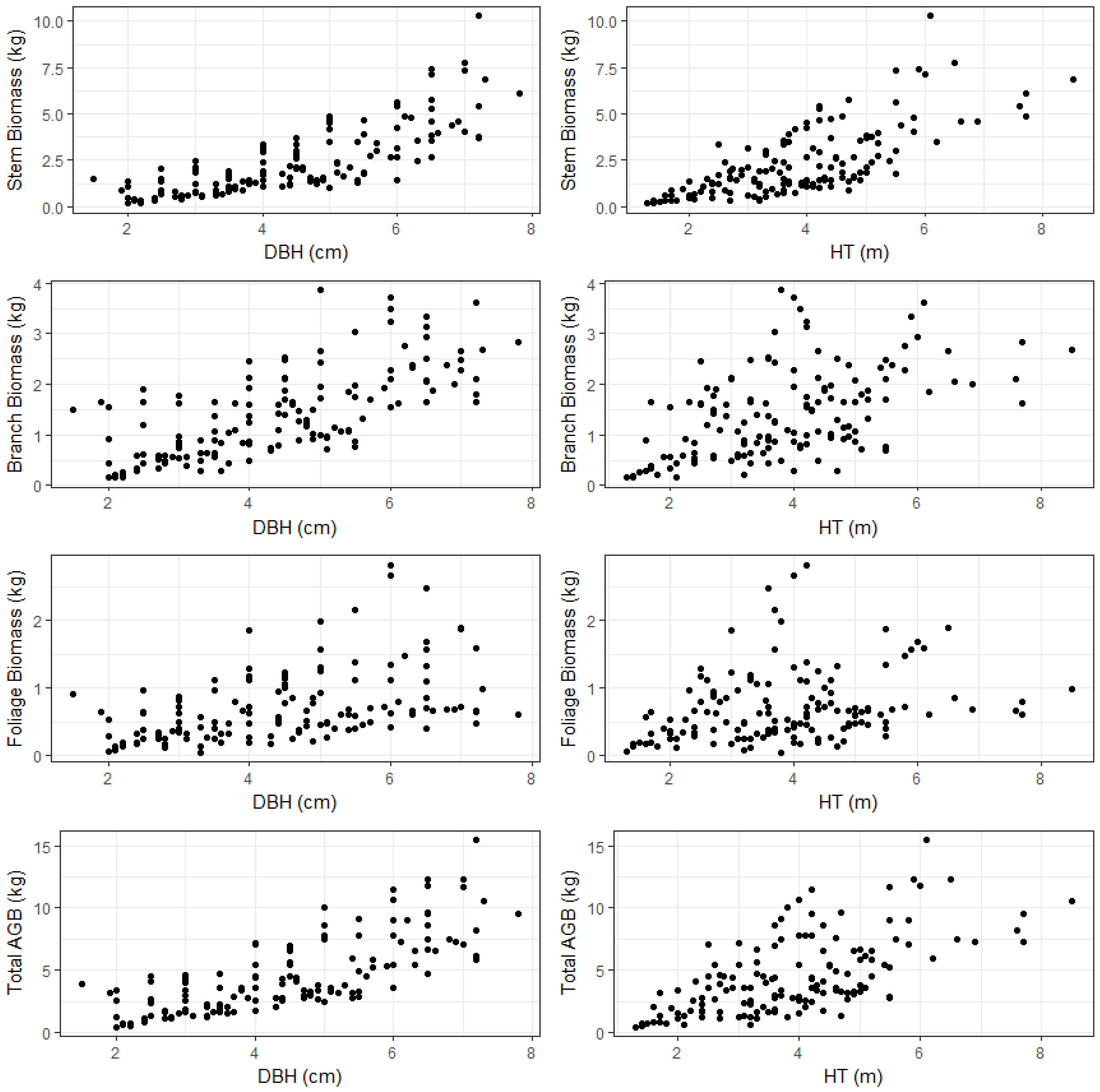
Representative sub-samples were taken from each biomass component to determine fresh to oven-dried biomass ratios. For each tree, after all the branches were separated, the whole stem was measured and cut with a chainsaw into 1 m long sections. Lost sawdust mass during tree and stem cutting or other sections was neglected because it was generally less than 0.03 kg per tree. To avoid the losses, newly sharpened chainsaws and axes were used in partitioning stem and branches. Subsequently, discs were (5 cm thick) cut and taken from the stem section at 1 m regular intervals along the full length of stem. Additional stem discs were also taken from the previously marked gravity center of the boles in order to guarantee reliable results. For branch and foliage, four 10–15 cm branch sub-samples were immediately taken from the representative branches at the center of gravity of crown and from different parts of the tree, distributed evenly within the crown based on a randomized branch sampling procedure. Half of the branch sub-samples were further stripped of all needles in order to determine foliage to branch biomass ratio. Discs and representative sub-samples of branch and foliage were then weighed and taken to the laboratory. Discs taken from the stem were oven dried at 104 °C until constant weight for a minimum of two days depending on the amount of sample. Foliage and branches were dried at 65 °C until constant weight for at least two days. After drying, sub-samples of the biomass components (discs, branches, and foliage) were reweighed to determine the average fresh to oven-dried biomass ratio which was later applied to convert fresh biomass into dry biomass for each component as well as for the whole tree. The summary statistics of DBH, height, age, total and component dry weights (biomass) are given in Table 1. In Figure 1, the values of each of the biomass components and total AGB are plotted against the tree level variables of DBH and tree height. This figure indicates that, for a given tree height, there is a large variation in the component and total biomass values.
2.2. Data Analysis
A two-step process was used to estimate AGB and its components. In the first step, a model to predict total AGB was fitted and in the second step, models to predict the proportions of biomass in different components were fitted. The methods used in each step are discussed below.
2.2.1. Estimating AGB
DBH is the most commonly used predictor variable of AGB. However, including height in addition to DBH improves the accuracy of such models [8,23]. A variety of model forms such as power function (e.g., Picard et al. [23]), simple logarithmic model resulting from logarithmic transformation of power function (e.g., Poudel and Temesgen [9]), and exponential model (e.g., Ritchie et al. [24]; Poudel and Temesgen [8]) have been used to relate such dendrometric variables to AGB. A simple linear model in the form of Equation (1) was first tested.
where is the total aboveground biomass of tree; , , and are regression parameters to be estimated from the data; is the diameter at breast height of the tree; is the height of tree, and is the random error.
The regression coefficient for height (estimate of in Equation (1)) was not statistically significant (p-value = 0.514). A logarithmic model in the form of Equation (2) was then tested.
where is the natural log and all other variables are the same as defined previously.
Parameters , , and in Equations (1) and (2) are not necessarily the same. Coefficient of height was still not statistically significant (p-value = 0.237). Scatterplots of DBH and height against AGB, however, did not show severe departure from the linear relationship (Figure 1). In addition, power and exponential models were also deemed insufficient.
Data for this study originated from 11 research plots installed in natural stands. Thus, our dataset has a hierarchical nature and trees within a plot have more similar allometry than trees from different plots. Analysis of such a dataset is best done by separating variance due to the plots using mixed effects models. Therefore, a nonlinear mixed model in the form of Equation (3) was selected as the final model for predicting AGB using DBH and tree height. All the regression coefficients of this model were statistically significant at the 0.05 level of significance. In addition, the likelihood ratio test indicated that the random effect was warranted .
where is the total aboveground biomass of tree in plot; is the random plot effect and ; is the diameter at breast height of the tree in plot; is the height of tree in plot. In addition, is independent of .
2.2.2. Estimating Component Biomass
Traditionally, the amount of biomass present in different tree components has been modeled using similar equations as the models used to predict total tree biomass. To ensure the additivity of such equations, the constrained seemingly unrelated regression has been popular. Recently, component biomass has been estimated as the product of predicted proportion obtained from different generalized linear models [5,8,9,25] and the predicted total biomass obtained from the method described in the previous section. In this study, the proportion of biomass in different tree components was estimated using three generalized linear models: beta regression, Dirichlet regression, and multinomial logistic regression. Biomass in different components was obtained as the product of predicted proportions and the total AGB obtained from Equation (3).
Beta Regression
Selection of a regression method depends on the type of the dependent variable. Proportions of component biomass, the dependent variables in our study, are continuous and restricted to the (0, 1) interval. In linear regression, the dependent variable is assumed to have a distribution following a normal distribution making it unsuitable for modeling proportions. Beta regression, introduced by Ferrari and Cribari-Neto [26], assumes that the dependent variables are beta distributed. The beta distribution is a continuous distribution defined on the unit interval. It has been used in forestry to model percent canopy cover [27], riparian percent shrub cover [28], component biomass proportions [5,8,9], and to model basal area mortality due to fire [29].
With mean and precision parameters defined as and respectively, Ferrari and Cribari-Neto [26] defined beta density function as:
where .
The beta regression model can then be written as:
where is a strictly increasing and double differentiable link function that maps (0, 1) in to the real line , is a vector of explanatory variables, is a vector of unknown unknown regression parameters (, and is a linear predictor (i.e., , usually for all so that the model has an intercept) [26].
Beta regression is a generalized linear model and different link functions are available to link the dependent variable with the linear predictor. A logit link function, was used, thus the predicted proportions are obtained as . The beta regression was performed in R 3.4.1 [30] with function betareg in the library betareg [26].
Dirichlet Regression
In Dirichlet regression, the dependent variable is assumed to follow a Dirichlet distribution which is a multivariate generalization of the beta regression. Therefore, it is useful when the dependent variable is a vector of proportions that represent the components as percentage of the total, thus the component proportions sum to 1. In forestry, it has been used to model component biomass [8,9,25,31] and to assess the potential of using photogrammetric data for species-specific forest inventories [32].
Maier [33] used similar parameterization of Ferrari and Cribari-Neto [26] to represent the Dirichlet distribution as follows:
where ( and are mean and precision parameters respectively); are the shape parameters for each components, , , and is the multinomial beta function. The regression model for mean is formulated as follows:
where is the link-function and again with the logit link function, the predicted values are calculated as for reference component and for other components. For the details on parameterization of the Dirichlet distribution and the method of parameter estimation in Dirichlet regression, refer to Maier [33]. The Dirichlet regression was performed in R 3.4.1 [30] with function DirichReg in the library DirichletReg [33] using component stem biomass as a reference group.
Multinomial Logistic Regression
The multinomial logistic regression provides the conditional probabilities of observing different components [34] and can be considered as the proportion of biomass in each component and estimated by model parameters [35]. The conditional probabilities of each component assuming component stem biomass as reference category are given by Equations (8)–(10). The multinomial logistic regression has been used by Poudel and Temesgen [8] to estimate the proportions of component biomass in Douglas-fir and lodgepole pine, by Poudel and Temesgen [9] to estimate biomass proportions in red alder and western hemlock, and by Huff et al. [36] to estimate proportion of biomass in different fuel class categories.
where , and are proportions of aboveground biomass in stem, branch, and foliage respectively; = DBH; = total tree height; and are model parameters. The multinomial logistic regression was performed in R 3.4.1 [30] with function multinomial in the library net with biomass present in each component was used as frequency weight.
2.3. Evaluation
Performances of all the methods were evaluated based on the bias (mean difference in observed and predicted values), bias percent, root mean squared error (RMSE), and RMSE percent produced by each method.
where n is the number of trees, and are observed and predicted values of AGB or its component, and is the mean AGB or component biomass.
3. Results and Discussion
Parameter estimates and their standard errors for the nonlinear mixed effects model used to predict total AGB are given in Table 2. The boxplot of AGB in each plot shows the variability in total AGB among 11 plots (Figure 2).
The relationship between AGB and dendrometric variables such as DBH and height varies by stands or plots. Therefore, the mixed effects model was appropriate in our study because it addressed the hierarchical nature of the data by incorporating plot level variation in the model. The bias and RMSE of this model for the modeling data were −0.01 kg and 0.84 kg (−0.17% and 18.84% of mean AGB, respectively). The residual analysis did not show any problems with the model fit (Figure 3).
Allocation of component biomass is influenced by various site factors such as stand density, site productivity, competition at the tree level, soil characteristics such as texture and moisture content, and tree characteristics such as species and age [8]. In mature stands and trees, most of the biomass is contained in the main stem. For our sample trees, stem, branch, and foliage biomass, on average, accounted for 50%, 33%, and 17% of total AGB. Stem biomass ranged from 27% to 68%, branch biomass ranged from 18% to 53%, and foliage biomass ranged from 4% to 29% of total AGB. The proportion of stem biomass increased with increasing DBH and height (Figure 4). Similar findings for brutian pine were reported by de-Miguel et al. [12]. They found that the proportion of stem biomass is lower in small or young trees whereas the proportion of crown biomass diminishes as the tree grows. Note that the proportions in compositional data are inversely related, i.e., if the proportion of one component increases, the proportion of the other components decreases—also seen in Figure 4. Foliage biomass decreased with increasing diameter and height. However, the rate of decline in foliage biomass was higher with increasing height (in meter) than with increasing DBH (in centimeter). This could be because the vertical competition has more effect on crown biomass than the horizontal competition. Branch biomass proportion showed a similar trend as the foliage proportion. After 4 cm DBH and 4 m height, both branch and foliage biomass declined monotonically while the stem biomass increased monotonically. This can have both ecological significance as well as management implications. One such implication is assessing the potential for supplying branch and foliage biomass (the logging residues) for bioenergy production. Kuuluvainen [37] found that the proportion of stem biomass from total AGB increased from smaller to larger trees and then stabilized. This reflects, in line with the pipe-model theory [38], the increasing need for biomass allocation into stem at early stages of tree development until a balance between stem and crown biomass accumulation is achieved. The results are consistent with current biological knowledge on stand dynamics of light-demanding species. Brutian pine is managed under even-aged schedules and trees growing in such stands have longer stems and smaller crowns because of the competition for light.
In this study beta, Dirichlet, and multinomial logistic regressions were used to predict the proportion of biomass in stem, branch, and foliage. These are all generalized linear models and were unbiased in predicting biomass proportions. However, the prediction of proportion and error in proportion itself is not as relevant and requires that both estimates and error in biomass units are obtained. This can be obtained by applying predicted proportions to the total biomass obtained from AGB equation. This underscores the importance of developing the best possible model to obtain total AGB because partitioning an inaccurate AGB would provide inaccurate estimates of the component masses as well. On the other hand, accurate models to predict component biomass are essential to meet other purposes such as to assess availability of biomass feedstock. Therefore, biomass in different components was obtained by applying predicted proportions to AGB predicted from the nonlinear mixed effects model.
The beta regression models predicted proportion of biomass in stem, branch, and foliage independently of each other. Parameter estimates and their standard errors of beta regression models are given in Table 3.
Component models are generally not as good as the model to fit AGB. The model to predict branch biomass proportion had the smaller pseudo-R2 (0.1827) than the models to predict stem and foliage biomass. This is justified by the flatter smooth line observed in Figure 4. The stem and foliage proportion models had pseudo-R2 0.4245 and 0.4780, respectively. The evaluation statistics produced by the beta regression models are given in Table 4. Branch and stem biomass were over predicted by the beta regression models by 1.62% and 0.25% whereas the foliage biomass was under predicted by 2.93%. RMSEs for the beta models were 39.11%, 31.50%, and 18.77% for foliage, branch, and stem biomass estimation, respectively. Note that, even though the foliage model had a higher pseudo-R2 value than the branch model, it had a higher RMSE percent than the branch model.
Dirichlet regression assumes that the dependent variable is a vector of proportions with unit sum and follows a Dirichlet distribution which is a multivariate generalization of the beta distribution. Unlike in beta regression, component models are fitted simultaneously, thus ensuring the unit sum of the predicted proportions. Parameter estimates and their standard errors along with fit statistics are presented in Table 5. The biomass in stem was used as the reference group, hence there were no parameter estimates for stem biomass. One can change the reference group to obtain model coefficients for stem biomass. However, the component proportions estimated in such a manner would not necessarily have unit sum.
Similar to beta regression, the Dirichlet regression over predicted branch and stem biomass by 1.52% and 0.12% whereas the foliage biomass was under predicted by 2.36%. RMSEs produced by the Dirichlet regression (Table 6) were practically identical to that produced by the beta regression but the Dirichlet regression should be preferred to the beta regression due to the assurance of the desired additive property.
Multinomial logistic regression is similar to the Dirichlet regression in the sense that both fit the components simultaneously and ensures that the sum of predicted proportions is equal to one. Parameter estimates and their standard errors of the multinomial logistic regression are given in Table 7.
Multinomial logistic regression over predicted the biomass proportions for all components by no more than 0.2% (Table 8). It produced the smallest RMSEs, compared to both beta and Dirichlet regressions. However, these RMSEs were within 0.5% of each other.
4. Conclusions
Using the data collected by destructively sampling 143 trees in 11 research plots installed in natural stands that were 11 to 26 years old, total and component biomass of brutian pine trees in Turkey were modeled. Total AGB was modeled using a nonlinear mixed effects model which accounted for the variability among plots. The predicted total AGB was then distributed into different tree components using the predicted proportions obtained from generalized linear models.
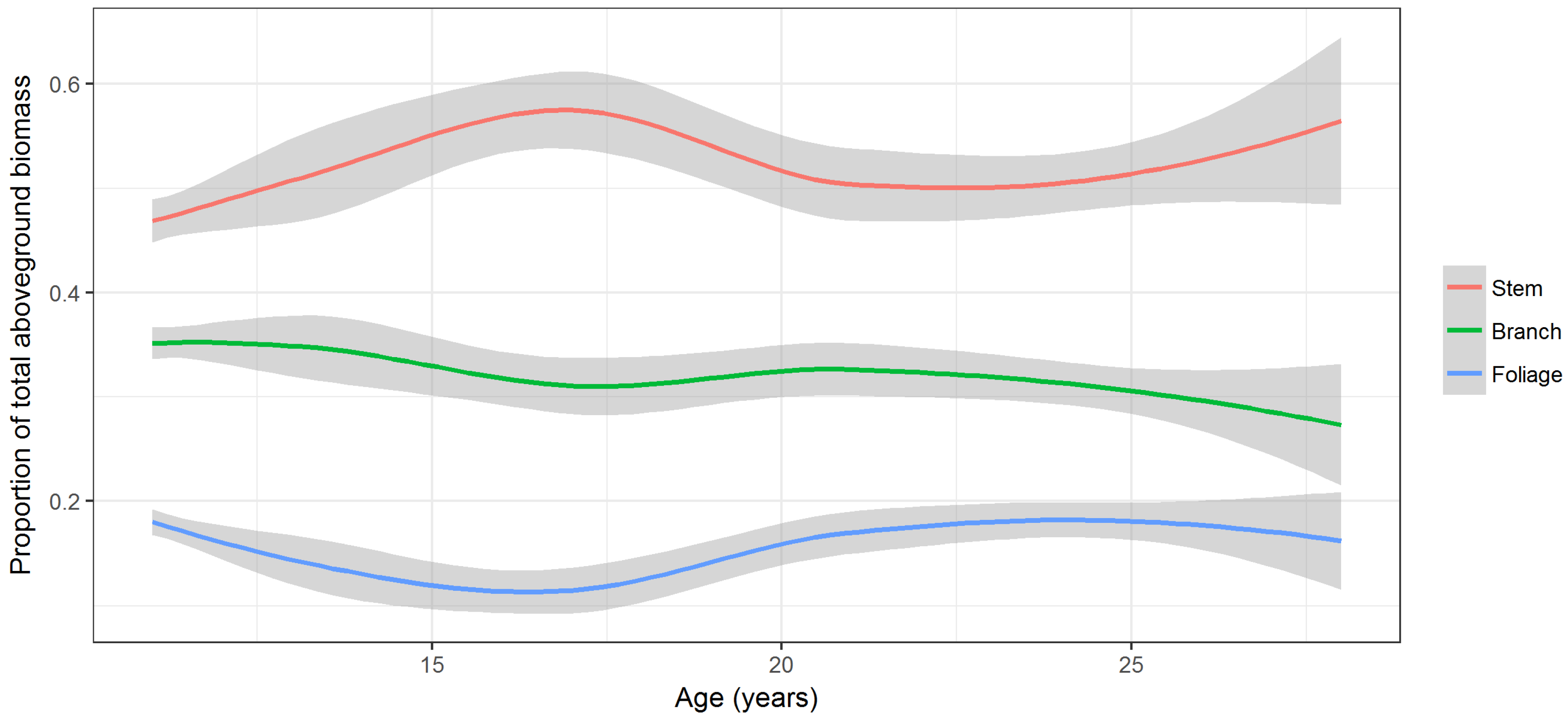
Stem, branch, and foliage biomass, on average, accounted for 50% (range 27–68%), 33% (range 18–53%), and 17% (range 4–29%) of total AGB. Biomass of different components did not follow a consistent trend with respect to tree age (Figure 5). Proportion of stem wood biomass increased until age 16 years, then declined until age 22 years, and increased again. Proportions of branch and foliage biomass declined until age 16, then increased until age 21, and declined again thereafter. The foliage proportion had a similar trend to the branch proportion but the second decline began after around age 25 years (Figure 5).
The beta, Dirichlet, and multinomial logistic regressions produced unbiased estimates of biomass proportions. These methods produced similar bias and root mean squared error values. The beta regression fits the component models independently. Therefore, it does not guarantee that the sum of the predicted proportions is equal to one. However, the Dirichlet and multinomial logistic regressions fit component models simultaneously and ensure the additivity of component masses. Note that the use of multinomial logistic regression requires arbitrary categorization and provides the predicted probabilities of those categories. In component biomass modeling, such predicted probabilities are considered the predicted proportions. The Dirichlet regression has the additive property, does not require such non-standard data categorization, and has similar performance as the multinomial logistic regression and may be preferred over the multinomial logistic regression. Models developed in this study can also be used in feasibility analysis of theoretical potential of establishing bioenergy plants, assessment of wildfire fuel load, and potential of brutian pine for carbon sequestration. Since the prediction accuracy of component biomass is dependent on the accuracy of the model to predict total AGB, future work on testing model forms and modeling approaches for AGB prediction with larger datasets is also critical.
Acknowledgments
This research was conducted within the scope of the project “Investigation on supply possibilities of logging residues” (Project No. 110O435), funded by Scientific and Technological Research Council of Turkey (TUBITAK). We are grateful to TUBITAK. A special thanks to all project members. We thank Bryce Frank of the Forest Measurement and Biometrics Lab at Oregon State University for providing diligent proofreading of the manuscript. Finally, we thank the anonymous reviewers of this article for their constructive comments, which have contributed to improving this manuscript.
Author Contributions
M.E. collected data and coordinated the research project; R.Ö. and K.P.P. analyzed data and co-wrote the results. M.E., R.Ö., and K.P.P. reviewed all results and wrote a draft. All authors discussed, revised, and designed the last version of the manuscript.
Conflicts of Interest
The authors declare no conflict of interest. The funding sponsors had no role in the design of the study; in the collection, analyses, or interpretation of data; in the writing of the manuscript, and in the decision to publish the results.
References
- GDF. Forestry Statistics–Wood Based Forest Products in Year of 2015. General Directorate of Forestry: Ankara. Available online: http://www.ogm.gov.tr/ekutuphane/Istatistikler/ (accessed on 20 February 2016).
- Bozkurt, A.Y.; Göker, Y. Forest Products Utilization; Istanbul University Press: Istanbul, Turkey, 1996. [Google Scholar]
- Fischer, R.; Lorenz, M.; Köhl, M.; Becher, G.; Granke, O.; Christou, A. The Condition of Forests in Europe: 2008 Executive Report; United Nations Economic Commission for Europe, Convention on Long-Range Transboundary Air Pollution, International Co-Operative Programme on Assessment and Monitoring of Air Pollution Effects on Forests (ICP Forests), Institute for World Forestry: Hamburg, Germany, 2008; p. 23. [Google Scholar]
- Dong, L.; Zhang, L.; Li, F. A compatible system of biomass equations for three conifer species in Northeast China. For. Ecol. Manag. 2014, 329, 306–317. [Google Scholar] [CrossRef]
- Zhou, X.; Hemstrom, M.A. Estimating Above-Ground Tree Biomass on Forest Land in the Pacific Northwest: a Comparison of Approaches; Res. Pap. PNW-RP-584; Department of Agriculture, Forest Service, Pacific Northwest Research Station: Portland, OR, USA, 2009; p. 18. [Google Scholar]
- Parresol, B.R. Assessing tree and stand biomass: A review with examples and critical comparisons. For. Sci. 1999, 45, 573–593. [Google Scholar]
- Parresol, B.R. Additivity of nonlinear biomass equations. Can. J. For. Res. 2001, 31, 865–878. [Google Scholar] [CrossRef]
- Poudel, K.P.; Temesgen, H. Methods for estimating aboveground biomass and its components for Douglas-fir and lodgepole pine trees. Can. J. For. Res. 2016, 46, 77–87. [Google Scholar] [CrossRef]
- Poudel, K.P.; Temesgen, H. Developing biomass equations for western hemlock and red alder trees in western Oregon forests. Forests 2016, 7, 88. [Google Scholar] [CrossRef]
- Durkaya, A.; Durkaya, B.; Atmaca, S. Predicting the above-ground biomass of Scots pine (Pinus sylvestris L.) stands in Turkey. Energy Source Part A Recovery Utili. Environ. Eff. 2009, 32, 485–493. [Google Scholar] [CrossRef]
- Zianis, D.; Xanthopoulos, G.; Kalabokidis, K.; Kazakis, G.; Ghosn, D.; Roussou, O. Allometric equations for aboveground biomass estimation by size class for Pinus brutia Ten. trees growing in North and South Aegean Islands, Greece. Eur. J. For. Res. 2011, 130, 145–160. [Google Scholar] [CrossRef]
- De-Miguel, S.; Pukkala, T.; Assaf, N.; Shater, Z. Intra-specific differences in allometric equations for aboveground biomass of eastern Mediterranean Pinus brutia. Ann. For. Sci. 2014, 71, 101–112. [Google Scholar] [CrossRef]
- Özçelik, R.; Diamantopoulou, M.J.; Eker, M.; Gürlevik, N. Artificial Neural Network Models: An Alternative Approach for Reliable Aboveground Pine Tree Biomass Prediction. For. Sci. 2017, 63, 291–302. [Google Scholar]
- Chaturvedi, R.K.; Raghubanshi, A.S. Aboveground biomass estimations of small diameter woody species of tropical dry forest. New For. 2013, 44, 509–519. [Google Scholar] [CrossRef]
- Daryaei, A.; Sohrabi, H. Additive biomass equations for small diameter trees of temperate mixed deciduous forests. Scand. J. For. Res. 2017, 31, 394–398. [Google Scholar] [CrossRef]
- Murray, R.B.; Jacobson, M.Q. An evaluation of dimension analysis for predicting shrub biomass. J. Range Manag. 1982, 35, 451–454. [Google Scholar] [CrossRef]
- Singh, V.; Tewari, A.; Kushwaha, S.P.S.; Dadhwal, V.K. Formulating allometric equations for estimating biomass and carbon stock in small diameter trees. For. Ecol. Manag. 2011, 261, 1945–1949. [Google Scholar] [CrossRef]
- Nelson, A.S.; Weiskittel, A.R.; Wagner, R.G.; Saunders, M.R. Development and evaluation of aboveground small tree biomass models for naturally regenerated and planted species in eastern Maine, U.S.A. Biomass Bioenergy 2014, 68, 215–227. [Google Scholar] [CrossRef]
- Schuler, J.; Bragg, D.C.; McElligott, K. Biomass estimates of small diameter planted and natural–origin Loblolly pines show major departures from the National biomass estimator equations. For. Sci. 2017, 63, 319–330. [Google Scholar] [CrossRef]
- Küçük, Ö.; Bilgili, E. Crown fuel load for young Calabrian pine (Pinus brutia Ten.) trees. Kastamonu Univ. J. Fac. For. 2007, 7, 180–189. [Google Scholar]
- Bilgili, E.; Küçük, O. Estimating above-ground fuel biomass in young Calabrian pine (Pinus brutia Ten.). Energy Fuels 2009, 23, 1797–1800. [Google Scholar] [CrossRef]
- Boydak, M. Silvicultural characteristics and natural regeneration of Pinus brutia Ten.—A review. Plant Ecol. 2004, 171, 153–163. [Google Scholar] [CrossRef]
- Picard, N.; Rutishauser, E.; Ploton, P.; Ngomanda, A.; Henry, M. Should tree biomass allometry be restricted to power models? For. Ecol. Manag. 2015, 353, 156–163. [Google Scholar] [CrossRef]
- Ritchie, M.W.; Zhang, J.; Hamilton, T.A. Aboveground tree biomass for Pinus ponderosa in northeastern California. Forests 2013, 4, 179–196. [Google Scholar] [CrossRef]
- Dahlhausen, J.; Uhl, E.; Heym, M.; Biber, P.; Ventura, M.; Panzacchi, P.; Tonon, G.; Horváth, T.; Pretzsch, H. Stand density sensitive biomass functions for young oak trees at four different European sites. Trees 2017, 31, 1–16. [Google Scholar] [CrossRef]
- Ferrari, S.; Cribari-Neto, F. Beta regression for modelling rates and proportions. J. Appl. Stat. 2004, 31, 799–815. [Google Scholar] [CrossRef]
- Korhonen, L.; Korhonen, K.T.; Stenberg, P.; Maltamo, M.; Rautiainen, M. Local models for forest canopy cover with beta regression. Silva Fenn. 2007, 41, 671. [Google Scholar] [CrossRef]
- Eskelson, B.N.; Madsen, L.; Hagar, J.C.; Temesgen, H. Estimating Riparian understory vegetation cover with Beta regression and copula models. For. Sci. 2011, 57, 212–221. [Google Scholar]
- Hoe, M.S. Multi-Temporal Lidar Analysis of Landscape Fire Effects in Southwestern Oregon. Master’s Thesis, Oregon State University, Corvallis, OR, USA, 2016; p. 162. [Google Scholar]
- R Core Team. A Language and Environment for Statistical Computing. Available online: http://www.R-project.org/ (accessed on 4 August 2017).
- Zhao, D.; Kane, M.; Teskey, R.; Markewitz, D. Modeling aboveground biomass components and volume-to-weight conversion ratios for loblolly pine trees. For. Sci. 2016, 62, 463–473. [Google Scholar] [CrossRef]
- Puliti, S.; Gobakken, T.; Ørka, H.O.; Næsset, E. Assessing 3D point clouds from aerial photographs for species-specific forest inventoires. Scand. J. For. Res. 2017, 32, 68–79. [Google Scholar] [CrossRef]
- Maier, M.J. DirichletReg: Dirichlet Regression for Compositional Data in R. Available online: http://epub.wu.ac.at/4077/ (accessed on 29 January 2014).
- Hosmer, D.W.; Lemeshow, S.; Sturdivant, R.X. Applied Logistic Regression, 3rd ed.; John Wiley & Sons Inc.: New York, NY, USA, 2013; p. 529. [Google Scholar]
- Boudewyn, P.; Song, X.; Magnussen, S.; Gillis, M. Model-Based, Volume to Biomass Conversion for Forested and Vegetated Land in Canada; Information Report BC-X-411; Natural Resources Canada, Canadian Forest Service, Pacific Forestry Centre: Victoria, BC, Canada, 2007. [Google Scholar]
- Huff, S.; Ritchie, M.; Temesgen, H. Allometric equations for estimating abovegorund biomass for common shrubs in northeastern California. For. Ecol. Manag. 2017, 398, 48–63. [Google Scholar] [CrossRef]
- Kuuluvainen, T. Relationships between crown projected area and components of above-ground biomass in Norway spruce trees in even-aged stands: Empirical results and their interpretation. For. Ecol. Manag. 1991, 40, 243–260. [Google Scholar] [CrossRef]
- Makela, A. Implications of the pipe model theory on dry matter partitioning and height growth in trees. J. Theor. Biol. 1986, 123, 103–120. [Google Scholar] [CrossRef]
Figure 1.
Sample trees of each of biomass component and total aboveground biomass (AGB) versus tree level variables for analyzed tree species. DBH and HT are diameter at breast height (cm) and total tree height (m).
Figure 1.
Sample trees of each of biomass component and total aboveground biomass (AGB) versus tree level variables for analyzed tree species. DBH and HT are diameter at breast height (cm) and total tree height (m).

Figure 2.
Boxplot of aboveground biomass in different plots in which the samples were destructively collected.
Figure 2.
Boxplot of aboveground biomass in different plots in which the samples were destructively collected.
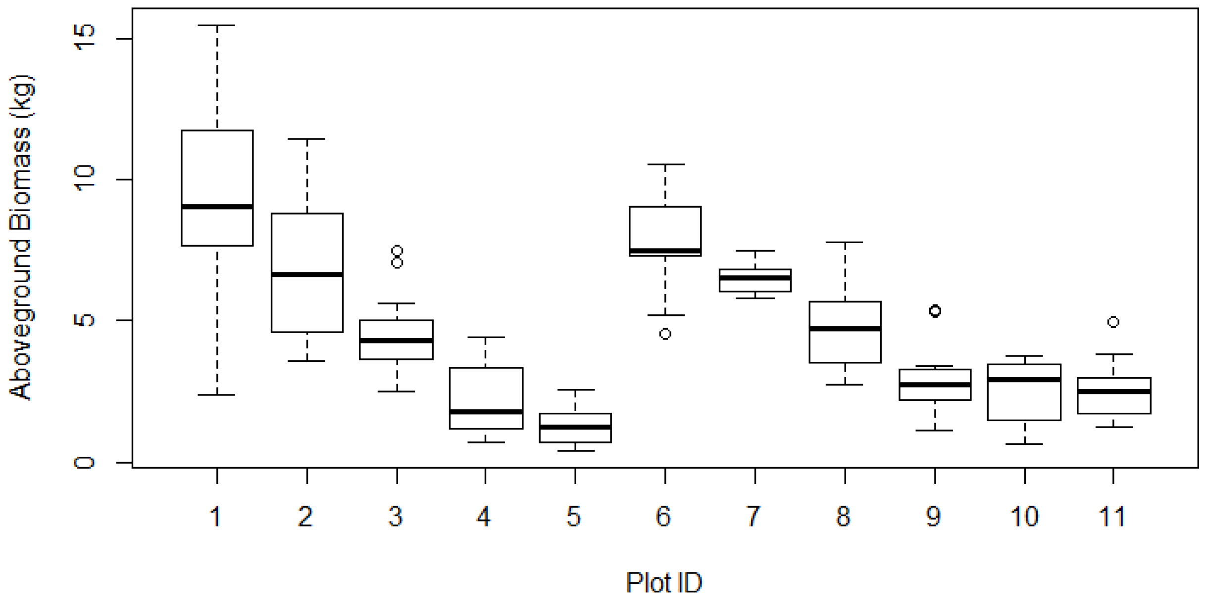
Figure 3.
Scatter plots of fitted values against the standardized residual of the model for predicting total aboveground biomass.
Figure 3.
Scatter plots of fitted values against the standardized residual of the model for predicting total aboveground biomass.
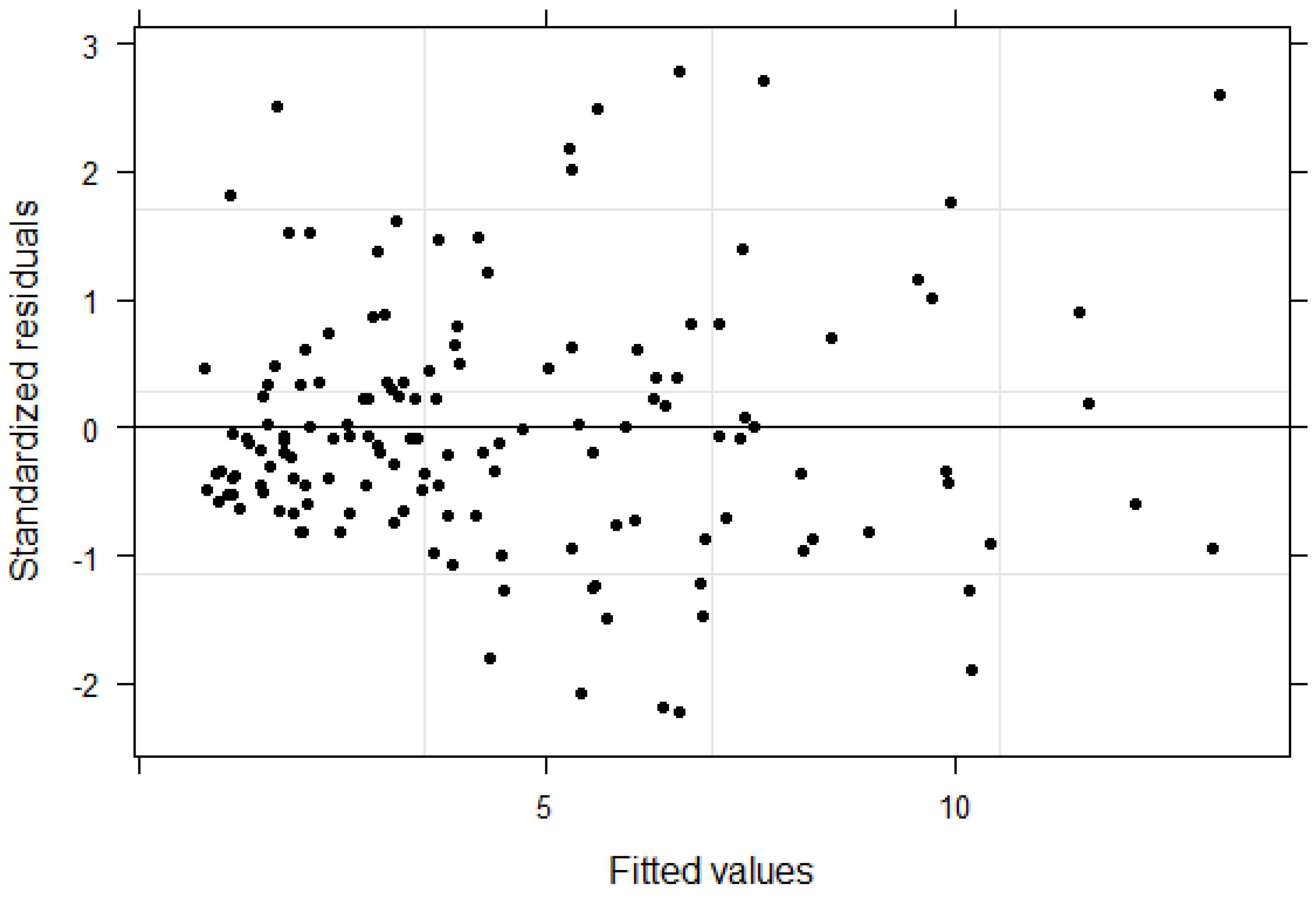
Figure 4.
Trend in component biomass proportion with respect to DBH and total height. Trend lines are obtained through loess fit.
Figure 4.
Trend in component biomass proportion with respect to DBH and total height. Trend lines are obtained through loess fit.
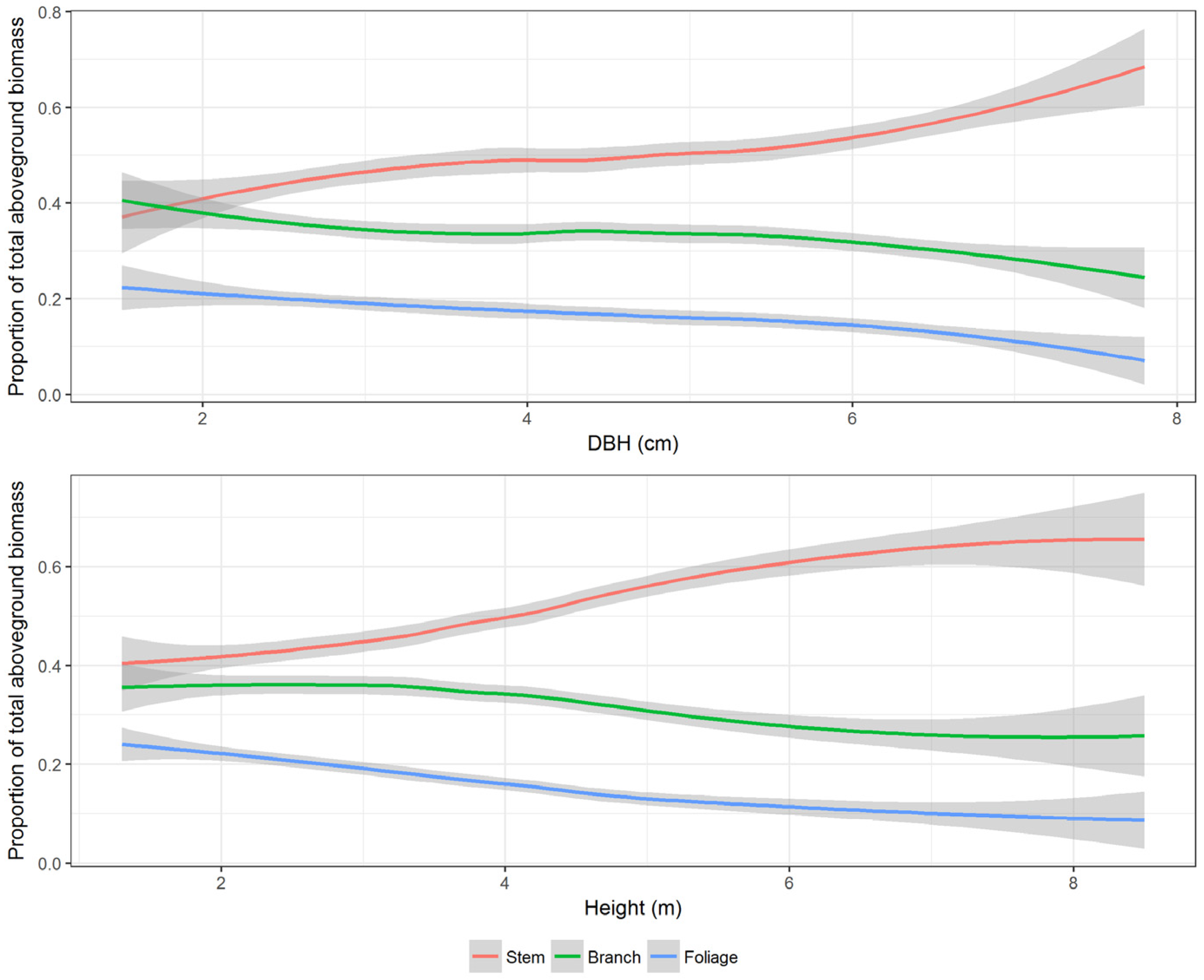
Figure 5.
Distribution of biomass in different aboveground components by age in small diameter brutian pine trees sampled in this study.
Figure 5.
Distribution of biomass in different aboveground components by age in small diameter brutian pine trees sampled in this study.


Table 1.
Summary statistics of sample trees used in estimating total aboveground biomass and its components.
Table 1.
Summary statistics of sample trees used in estimating total aboveground biomass and its components.
| Variables | n | Minimum | Maximum | Mean | Standard Deviation |
|---|---|---|---|---|---|
| DBH | 143 | 1.50 | 7.8 | 4.40 | 1.53 |
| HT | 143 | 1.30 | 7.70 | 3.86 | 1.42 |
| AGE | 143 | 11.00 | 26.00 | 14.87 | 4.68 |
| AGB | 143 | 0.42 | 15.48 | 4.45 | 3.03 |
| STM | 143 | 0.18 | 10.29 | 2.32 | 1.85 |
| BCH | 143 | 0.15 | 3.86 | 1.42 | 0.86 |
| FOL | 143 | 0.05 | 2.82 | 0.71 | 0.52 |
DBH, diameter at breast height (cm); HT, total tree height (m); AGE, age in years; AGB, aboveground biomass (kg); STM, stem biomass (kg); BCH, branch biomass (kg); FOL, foliage biomass (kg).
Table 2.
Parameter estimates and their standard errors for the model used to predict total AGB (Equation (3)) of small DBH trees. are regression coefficients and and are variance components of mixed models.
Table 2.
Parameter estimates and their standard errors for the model used to predict total AGB (Equation (3)) of small DBH trees. are regression coefficients and and are variance components of mixed models.
| Coefficient | Estimate | Standard Error |
|---|---|---|
| −0.99599 | 0.17875 | |
| 1.19234 | 0.10157 | |
| 0.44547 | 0.11328 | |
| 0.87035 | ||
| 0.35789 |
Table 3.
Parameter estimates, their standard error (in parenthesis), and pseudo-R2 (an R2-like measure calculated based on estimated likelihood) values for the small DBH trees using beta regression.
Table 3.
Parameter estimates, their standard error (in parenthesis), and pseudo-R2 (an R2-like measure calculated based on estimated likelihood) values for the small DBH trees using beta regression.
| Model | Parameter Estimates | pseudo-R2 | ||
|---|---|---|---|---|
| Intercept | DBH | HT | ||
| Foliage | −0.91797 (0.07839) | 0.06866 (0.03182) | −0.26256 (0.03567) | 0.4245 |
| Branch | −0.35913 (0.07030) | 0.01450 (0.02795) | −0.10239 (0.03045) | 0.1827 |
| Stem | −0.68726 (0.07219) | −0.04483 (0.02826) | 0.22690 (0.03089) | 0.4780 |
Table 4.
Bias and root mean squared error (RMSE) obtained from beta regression.
| Component | Bias (kg) | Bias Percent | RMSE (kg) | RMSE Percent |
|---|---|---|---|---|
| Foliage | 0.0207 | 2.9291 | 0.2764 | 39.1106 |
| Branch | −0.0230 | −1.6228 | 0.4464 | 31.4956 |
| Stem | −0.0059 | −0.2541 | 0.4357 | 18.7655 |
Table 5.
Parameter estimates for the component biomass models for small DBH trees using Dirichlet regression. Component stem biomass was used as the reference group.
Table 5.
Parameter estimates for the component biomass models for small DBH trees using Dirichlet regression. Component stem biomass was used as the reference group.
| Model | Parameter Estimates | R2 | ||
|---|---|---|---|---|
| Intercept | DBH | HT | ||
| Foliage | 0.16631 (0.07383) | 0.02972 (0.02884) | ‒0.17838 (0.03135) | 0.4602 |
| Branch | ‒0.16228 (0.09182) | 0.07570 (0.03647) | ‒0.32911 (0.04184) | 0.1880 |
Table 6.
Bias and root mean squared error obtained from Dirichlet regression.
| Component | Bias (kg) | Bias Percent | RMSE (kg) | RMSE Percent |
|---|---|---|---|---|
| Foliage | 0.0167 | 2.3631 | 0.2763 | 39.0965 |
| Branch | ‒0.0216 | ‒1.5240 | 0.4468 | 31.5238 |
| Stem | ‒0.0028 | ‒0.1206 | 0.4351 | 18.7396 |
Table 7.
Parameter estimates for the component biomass models for small DBH trees using multinomial logistic regression model. Component stem was used as the reference group.
Table 7.
Parameter estimates for the component biomass models for small DBH trees using multinomial logistic regression model. Component stem was used as the reference group.
| Model | Parameter Estimates | R2 | ||
|---|---|---|---|---|
| Intercept | DBH | HT | ||
| Foliage | ‒0.10942 (0.41677) | 0.05607 (0.13695) | ‒0.31204 (0.14648) | 0.4516 |
| Branch | 0.28112 (0.33235) | ‒0.00041 (0.10719) | ‒0.17256 (0.10946) | 0.1766 |
Table 8.
Bias and root mean squared error obtained from multinomial logistic regression.
| Component | Bias (kg) | Bias Percent | RMSE (kg) | RMSE Percent |
|---|---|---|---|---|
| Foliage | ‒0.0004 | ‒0.0566 | 0.2744 | 38.8276 |
| Branch | ‒0.0017 | ‒0.1199 | 0.4395 | 31.0087 |
| Stem | ‒0.0055 | ‒0.2369 | 0.4309 | 18.5587 |
© 2017 by the authors. Licensee MDPI, Basel, Switzerland. This article is an open access article distributed under the terms and conditions of the Creative Commons Attribution (CC BY) license (http://creativecommons.org/licenses/by/4.0/).
Share and Cite
MDPI and ACS Style
Eker, M.; Poudel, K.P.; Özçelik, R. Aboveground Biomass Equations for Small Trees of Brutian Pine in Turkey to Facilitate Harvesting and Management. Forests 2017, 8, 477. https://doi.org/10.3390/f8120477
AMA Style
Eker M, Poudel KP, Özçelik R. Aboveground Biomass Equations for Small Trees of Brutian Pine in Turkey to Facilitate Harvesting and Management. Forests. 2017; 8(12):477. https://doi.org/10.3390/f8120477
Chicago/Turabian StyleEker, Mehmet, Krishna P. Poudel, and Ramazan Özçelik. 2017. "Aboveground Biomass Equations for Small Trees of Brutian Pine in Turkey to Facilitate Harvesting and Management" Forests 8, no. 12: 477. https://doi.org/10.3390/f8120477
Note that from the first issue of 2016, this journal uses article numbers instead of page numbers. See further details here.