Article

Accuracy of Photogrammetric UAV-Based Point Clouds under Conditions of Partially-Open Forest Canopy

Department of Forest management and Geodesy, Faculty of Forestry, Technical University in Zvolen, T.G. Masaryka 24, Zvolen 96053, Slovakia
*
Author to whom correspondence should be addressed.
Forests 2017, 8(5), 151; https://doi.org/10.3390/f8050151
Submission received: 20 December 2016 / Revised: 20 April 2017 / Accepted: 27 April 2017 / Published: 30 April 2017

Abstract

:
This study focuses on the horizontal and vertical accuracy of point-clouds based on unmanned aerial vehicle (UAV) imagery. The DJI Phantom 3 Professional unmanned aerial vehicle and Agisoft PhotoScan Professional software were used for the evaluation. Three test sites with differing conditions (canopy openness, slope, terrain complexity, etc.) were used for comparison. The accuracy evaluation was aimed on positions of points placed on the ground. This is often disregarded under forest conditions as it is not possible to photogrammetrically reconstruct terrain that is covered by a fully-closed forest canopy. Therefore, such a measurement can only be conducted when there are gaps in the canopy or under leaf-off conditions in the case of deciduous forests. The reported sub-decimetre horizontal accuracy and vertical accuracy lower than 20 cm have proven that the method is applicable for survey, inventory, and various other tasks in forests. An analysis of ground control point (GCP) quantity and configuration showed that the quantity had only a minor effect on the accuracy in cases of plots with ~1-hectare area when using the aforementioned software. Therefore, methods increasing quality (precision, accuracy) of GCP positions should be preferred over the increase of quantity alone.

1. Introduction

Unmanned aerial vehicles (UAVs), also known as unmanned aircraft systems (UAS) and remotely-piloted aircraft systems (RPAS, a subset of UAS excluding fully-autonomous systems), are a very promising technology for forestry practice. A gradually growing number of research papers focusing on UAV use for forestry can be witnessed in the past five years. A review study of Torresan et al. [1] focused on the use of UAVs within the European region in the field of forestry, reporting that RGB (red, green, blue) imaging is the most adopted technology used in combination with UAVs. The forest inventory and dendrometric parameters are primary research objects. The same applies if we extend the region to the whole world.
In forestry applications, researchers are focusing on the estimation of forest inventory and crown parameters [2,3,4,5,6,7,8,9,10,11], real-time and post-forest fire monitoring and detection [12,13,14], health status and disease monitoring [15,16,17], individual trees and species detection [18,19,20], or surveying the current state of soil displacement [21]. RGB or NIR (near infrared) cameras are used in the majority of these studies. Many other applications of UAVs have also been described apart from forestry, e.g., agriculture [22,23], damage detection of buildings [24,25], landslide research [26], research of coastal environments and wetlands [27,28], archaeology [29], wildlife research and management [30], and many others. Overall, the main advantages of the small UAVs are their relatively low price and ability to collect data with high spatial and temporal resolution on demand [31]. The main disadvantage is a short flight time and, therefore, a relatively small sensed area. Security and privacy issues must also be mentioned. Although these are not of main concern in forests, the resulting legal restrictions often complicate the use of UAVs (e.g., [32,33]). Additionally, problems with lowered visibility and shorter signal range must be taken into the account in forests.
Recent developments in the field of computers and computer vision have allowed the processing of a large amount of imaging data using so-called structure-from-motion (SfM) and multi-view stereopsis (MVS) techniques. In contrast to traditional digital photogrammetric methods, which require the information on the 3D position of the camera or the 3D location of multiple control points, the SfM approach requires neither of these for scene reconstruction. Camera pose and scene geometry are reconstructed simultaneously using the automatic identification and matching of features in multiple images [34]. This results in the alignment of the images and generation of a point cloud consisting of identical points, which can be subsequently densified. Ground control points (GCPs) are used for georeferencing of the point cloud. The point cloud, and eventually an orthomosaic, is scaled using the positions of GCPs, which are surveyed using an accurate method (e.g., GPS or total station measurements). The survey of GCPs is often more complicated under forest conditions compared to open-area conditions. The accuracy of the georeferencing process is crucial for any following analysis where accurate positions of, e.g., tree stems or crowns, are of high priority. Regarding recent studies on UAV applicability in forestry [2,3,4,5,12,15,18,20,21,35,36,37], five to 89 ground control points were used for georeferencing of point clouds based on RGB or NIR imagery. If the authors mentioned the accuracy of georeferencing, it ranged from a few centimetres to meters. The accuracy of UAV-based photogrammetric products is generally dependent on the platform (multirotor, fixed wing), camera specifications, flight altitude, structure and texture of the reconstructed surface, and applied software (e.g., [38,39]). Therefore, it is complicated to generalise results of studies regarding UAV applications.
The main aim of this study was to evaluate the accuracy of UAV-based point clouds under forest conditions with differing grades of tree cover. Only subsets of the point clouds related to terrain were included in the testing while excluding the above-ground biomass. Two main hypotheses were tested. First, the accuracy of terrain reconstruction, based on UAV-acquired imagery, is sufficient for tasks related to horizontal and vertical configurations of the terrain under forest conditions. Second, the quantity and configuration of ground control points has a significant influence on the resulting point cloud accuracy with regard to area and the applied software. An influence of terrain slope was also evaluated, although it was not the primary task of the study.

2. Materials and Methods

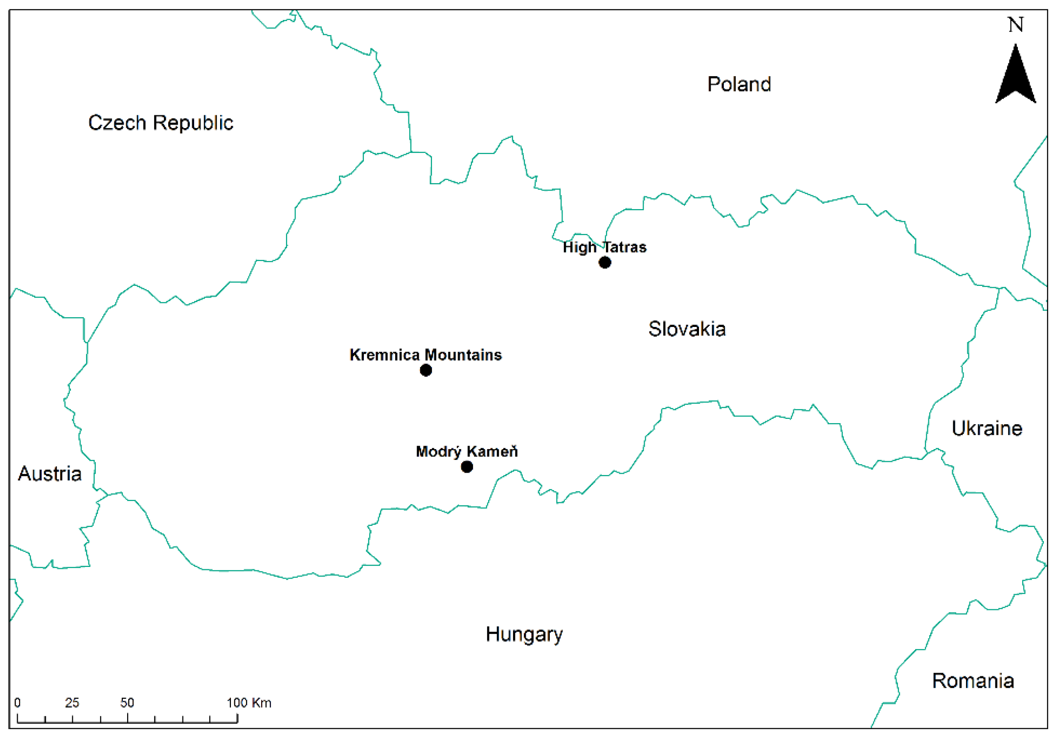
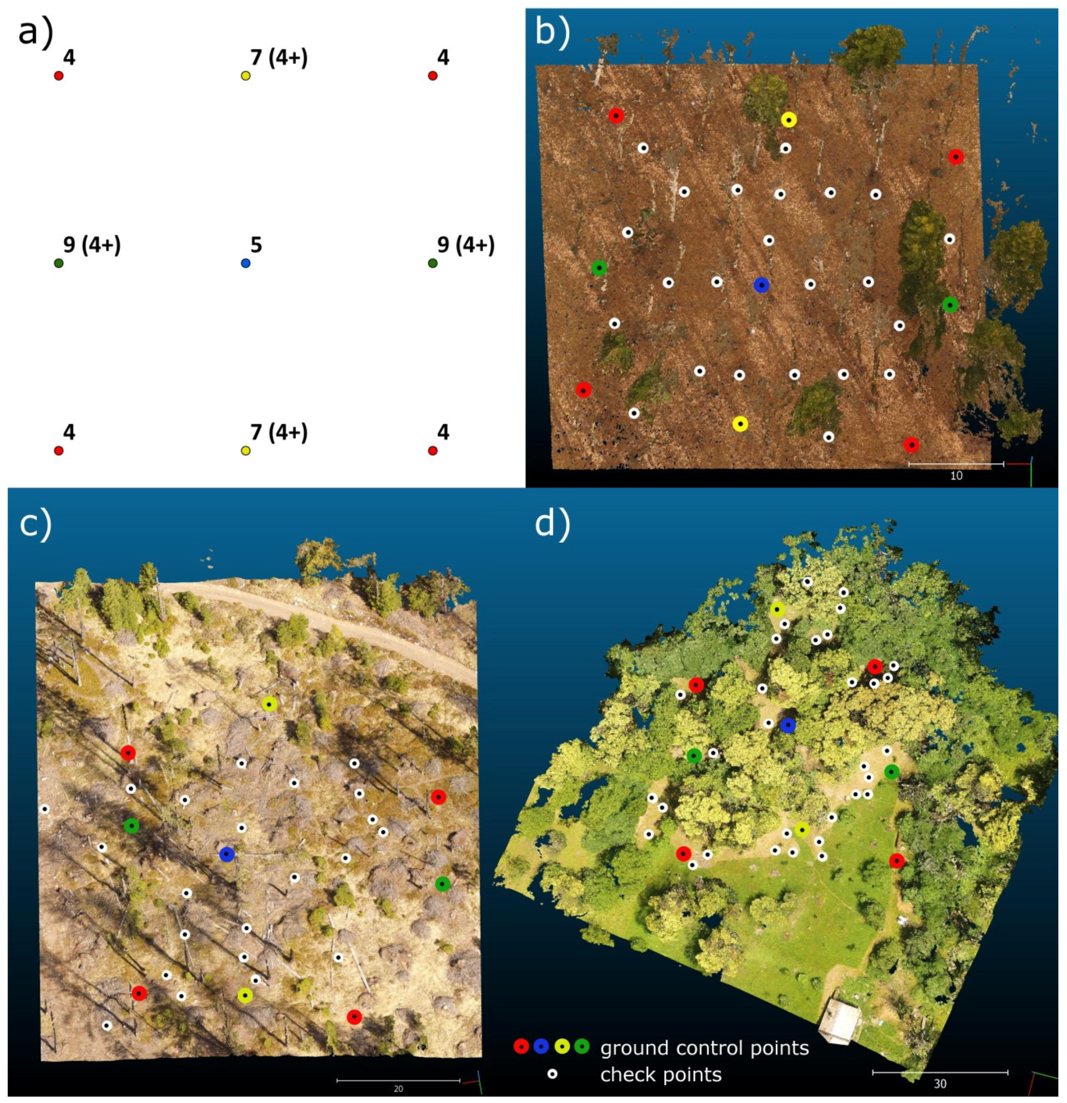
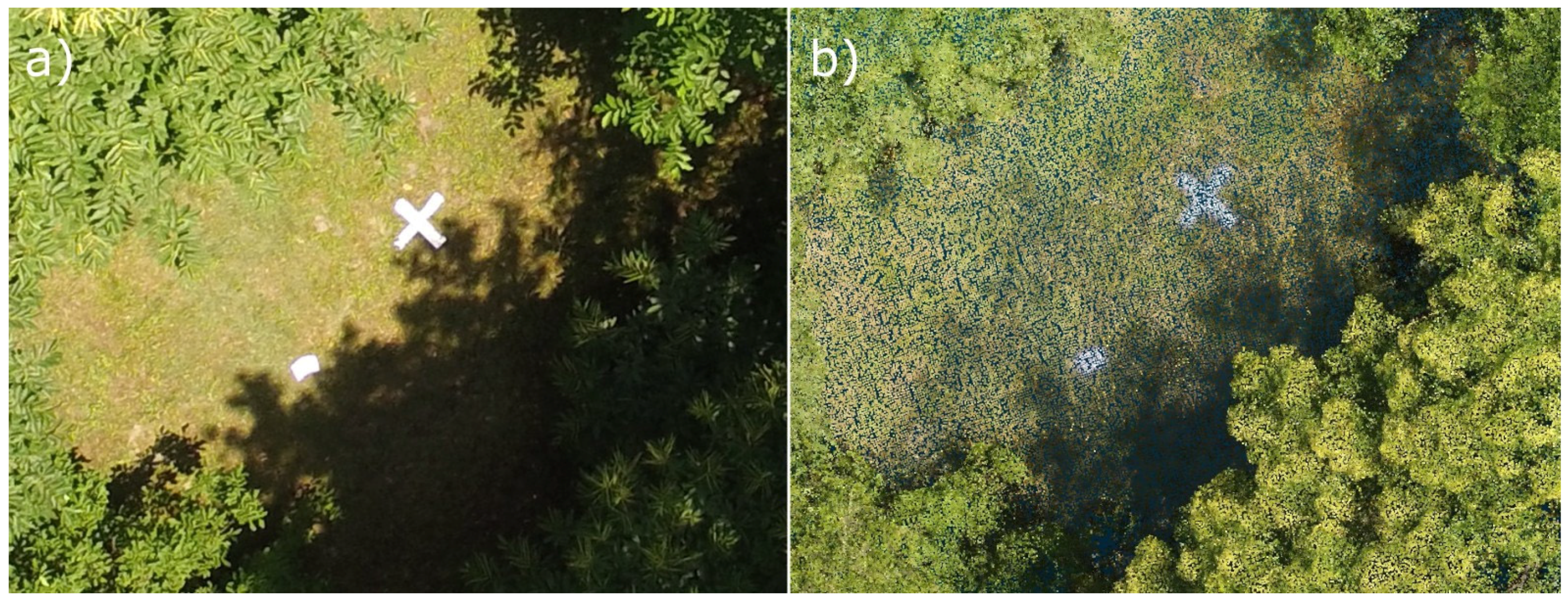
2.1. Study Sites and Reference Measurements

Three test plots were established within the Kremnica Mountains, the High Tatras Mountains, and in the vicinity of Modrý Kameň city (Figure 1). The plot in the Kremnica Mountains was established on 23 March 2016, the plot in the High Tatras was established on 21 April 2016, and the plot in Modrý Kameň was established on 14 September 2016.
The plots vary by tree cover, dominant tree species (>95%), tree age and height, slope, vegetation period, and height above sea level (AMSL) (Table 1). The plot in the Kremnica Mountains was established in a commercial forest stand with Fagus sylvatica (>95% representation) and Abies alba (<5% representation); the measurements were conducted during the leaf-off season. This plot represents flat terrain with minimal changes in microrelief, and the slope is minimal. In contrast to this test plot, the other two test plots were photographed during the leaf-on season. The plot in the High Tatras represents a forest stand damaged by wind disturbance in 2004, when most of the trees were damaged and cleared from the plot area. Just a few Larix decidua trees remain within the plot. In contrast to the Kremnica Mountains plot, the terrain is rugged with many changes in microrelief resulting from disturbances and the remaining coarse wood debris. The slope is moderate. The plot in Modrý Kameň is a chestnut garden (Castanea sativa) with a small amount of Juglans regia established on the edge of the city area. Some of the Castanea sativa specimens reach diameters at breast height as large as 1 m, while the thickest one is 1.497 m. A relatively high slope is typical for this plot, exceeding 40%. Other characteristics of the test plots are in Table 1.
Nine ground control points (GCP) were established at every test site using a 1 m × 1 m cross of white foil. Other checkpoints were signalled using white A4 paper with a nail in the centre (see Figure 2). As the GCPs and checkpoints were established with regard to visibility on the top-down imagery, the count of the checkpoints varies—23 points at the Kremnica Mountains site, 24 at the High Tatras site, and 32 at the Modrý Kameň site. Reference positions of GCPs and checkpoints were surveyed using a Topcon GPT-9000M total station (TOPCON Corporation, Tokyo, Japan). Three observation points were used at every site. The position of the observation points was determined using the GNSS RTK method (using a Topcon Hiper GGD survey-grade receiver (TOPCON Corporation, Tokyo, Japan)) to transform the measurements into the global coordinate system (WGS84) and, subsequently, to the Slovak national coordinate system S-JTSK, which was used in all following analyses.

2.2. UAV Imagery Acquisition and Processing

A DJI Phantom 3 Professional (DJI, Shenzhen, China) was used for imagery acquisition on all plots. The device is a commercial “all in one solution” quadcopter. In addition to the aircraft itself, it consists of a built-in camera with a three-axis gimbal, remote control, and a mobile application for the aircraft and camera control and the information about the state of the aircraft. The camera sensor is an RGB Sony Exmor 1/2.3″ CMOS with lens FOV of 94°, 20 mm focal length, f/2.8 focal ratio, and focus to infinite. Image resolution of the camera is 4000 × 3000 pixels.
The workflow of imagery acquisition followed the same pattern for each plot. The semi-autonomous flight option was used. A preliminary flight was necessary to plan the trajectory and acquire locations of waypoints (positions of the UAS) that are used during the semi-autonomous flight. Subsequently, the aircraft flies between these points with a given altitude, speed, and camera settings. These were specified with regard to the acquisition of at least 80% forward overlap and 60% lateral overlap between images. This is a drawback of the current version of the used application since, in previous versions, it was possible to design the flight plan without the preliminary flight using desired flight parameters and waypoints based on WGS84 coordinates. The necessity of the preliminary flight increases the number and time of flights as reported in Table 2. The flight altitude was proposed between 50 and 60 m, according to previous experience; the average flight speed was 0.5 m/s. This applies to the Kremnica and High Tatras sites. Since the elevation difference at Modrý Kameň is more than 50 m when also considering the covering vegetation, the 50 m flight altitude can be considered the average with ~25 m altitude over the highest parts and ~75 m over the lowest parts of the site.
The imagery was processed using Agisoft PhotoScan Professional 1.2.6 software (Agisoft LCC, St. Petersburg, Russia [40]). The camera was pre-calibrated using the Agisoft LENS software (Agisoft LCC, St. Petersburg, Russia), which uses a checker board to determine calibration parameters. As a dense point cloud was necessary for the subsequent analyses, only two steps of the entire workflow were applied. First, “Align Photos” was conducted using the “Accuracy” parameter set to “High” and “Pair preselection: Disabled”. When the “High” accuracy is chosen the original resolution of images is used. The pair preselection set to “Disabled” provides the most accurate image matching. The other options are “Generic” and “Reference”. The “Generic” setting is a two-step approach where a downscaling of imagery is applied. The “Reference” uses the geolocation of the images and, in the first step, the pairs are selected based on the position of images. Both options speed up the process, but decrease the accuracy. This is the reason why the “Disabled” option was chosen. The limit for key points was set to 40,000 and for tie points to 4000. The key point limit is the maximum number of points detected within each image and tie points limit is the number of points used for image matching. The reported values are the default. The second step, “Build dense cloud”, was conducted using the “Quality” parameter set to “High” and “Depth filtering” set to “Aggressive”. Three other options are provided for the “Depth filtering”. The “Aggressive” option is recommended for aerial imagery because it removes the highest number of outliers. Ground control points were included in the bundle adjustment; this resulted in proper scaling and transformation of the resulting point clouds to the S-JTSK coordinate system. The GCPs were identified on at least three photos, where the proximity to the image centre was considered to avoid further distortions near edges as the camera was pre-calibrated, and to sustain consistent methodology, because, especially on the Modrý Kameň site, some GCPs were visible only from the nadir. Five differing GCP configurations were used for every point cloud to evaluate an influence of GCP quantity and configuration on the resulting accuracy. First, two configurations consisted of four GCPs, where in the first one the GCPs were placed near corners of the point cloud, while in the other, the GCPs were placed near the middles of the sides. These two configurations are further referenced as four GCP “corner” and “cross” configurations. The other three configurations were designed using the addition of further points to the four GCP “corner” configuration. The sequence of the addition was: one point approximately in the middle of the point-cloud (five GCP configuration), two GCPs near the edges of the point-cloud in a direction of the highest slope (seven GCP configuration), and another two GCPs approximately in the direction of the contour lines (nine GCP configuration). A scheme of the GCP configurations, as well as actual location of GCPs and CPs, is shown in Figure 3.
The positions of the checkpoints were determined directly on the point clouds after every transformation. After identifying and clicking the centre of the mark, the Photoscan software snapped the position to the nearest point. Coordinates (X, Y, Z) of these points were exported in .txt format and used for subsequent analyses.

2.3. Statistical and Spatial Analysis

The coordinates of points, acquired from point clouds using the aforementioned method, were compared to the reference using following measures:
Calculation of the root mean square coordinate errors is as follows:
R M S E x = i = 1 n Δ x i 2 n
R M S E y = i = 1 n Δ y i 2 n
R M S E z = i = 1 n Δ z i 2 n
where Δxi, Δyi, and Δzi are the differences between reference coordinates and the coordinates determined from the point cloud, and n is the number of points in the set. Minima, maxima, means, and standard deviations were calculated for Δzi to enable a more detailed analysis of the vertical accuracy. The RMSEx and RMSEy errors were used for the calculation of the root mean square horizontal error RMSExy as follows:
R M S E x y = R M S E x 2 + R M S E y 2
The RMSExy is one of the most common horizontal accuracy criteria for sets of points and was used for the comparison between the test sites and between various configurations of GCPs. A variation of the F-test, the so-called “coefficient of relative efficiency”, was used as a measure of statistical significance of differences between the test sites. It is calculated as follows [41]:
R e = R M S E A 2 R M S E B 2
The RMSEA represents the mean error with a higher value, while RMSEB is the mean error with a lower value. The resulting value is compared to the upper critical value of the F-distribution. The critical values are shown in Table S1 (Suplementary Materials).
A second measure of the horizontal accuracy—positional error of individual points, Δp—was used because the RMSExy errors do not provide detailed information on the within-group variability. This error, representing a distance between the point cloud-based position of a point and the reference position was determined using the following equation:
Δ p i = Δ x i 2 + Δ y i 2
Minima, maxima, means, and standard deviations of the positional errors were calculated for every GCP configuration. A one-way ANOVA with a post-hoc Tukey HSD test was used to determine the statistical significance of differences between groups representing the differing GCP configurations. This test was used for the elevation errors Δzi, as well as the positional errors Δpi. Even though normality tests have not proven the normality of some groups, we present the results of the parametric ANOVA as we consider the means and standard deviations suitable for a description of the groups. The ANOVA and normality tests were conducted using STATISTICA software (Statsoft Inc., Tulsa, OK, USA [42]).
In addition to the statistical analysis, the spatial analysis of the error distribution was also conducted using QGIS 2.16 software (open-source software [43]). The distribution of errors on CPs was interpolated using an inverse distance weighting method and visually evaluated. The errors on GCPs were not included. The changes of the point clouds resulting from differing GCP configurations were also evaluated using CloudCompare software (open-source software [44]). The nearest-neighbour absolute cloud-to-cloud distances were computed and graphically displayed.

3. Results

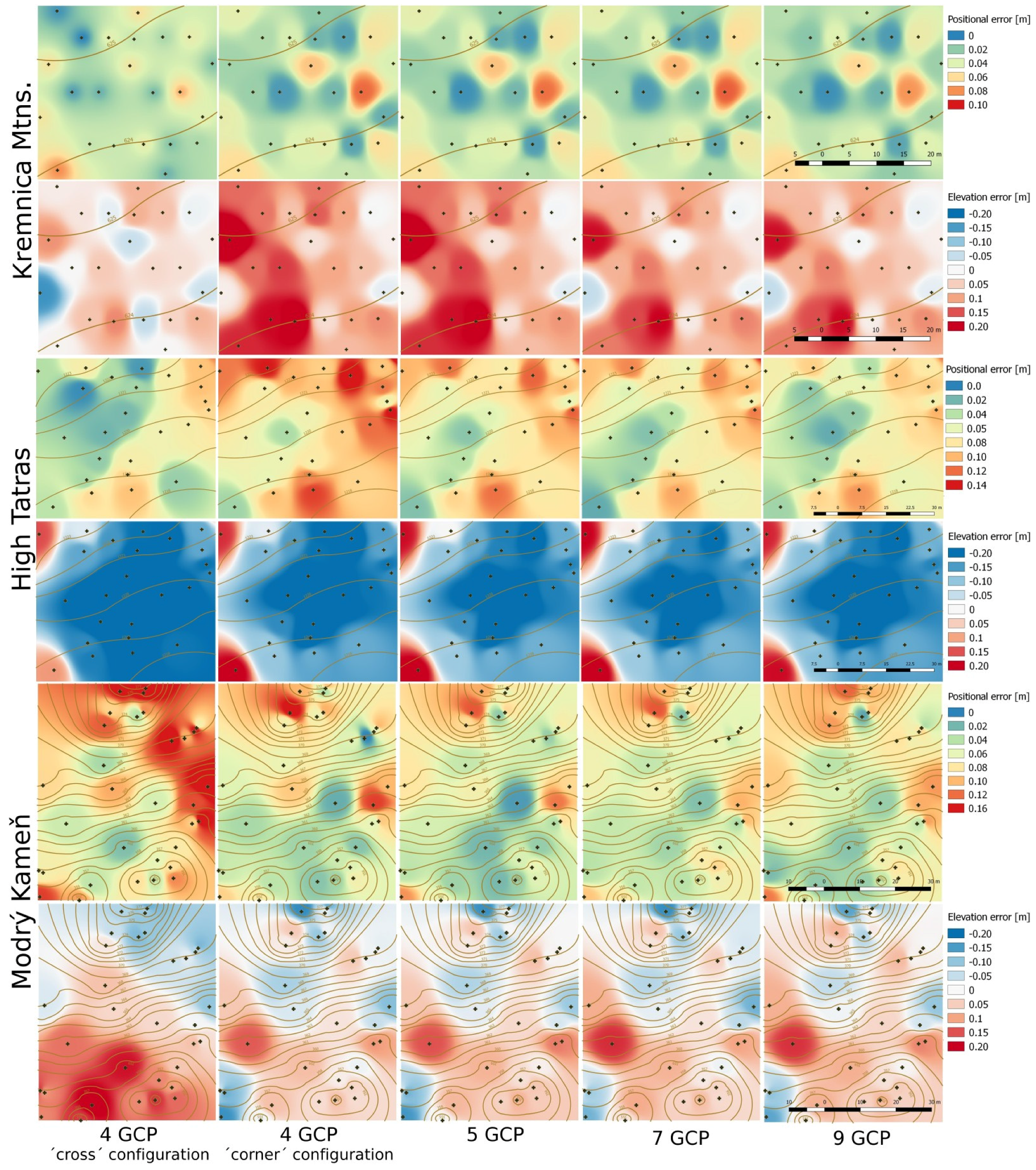
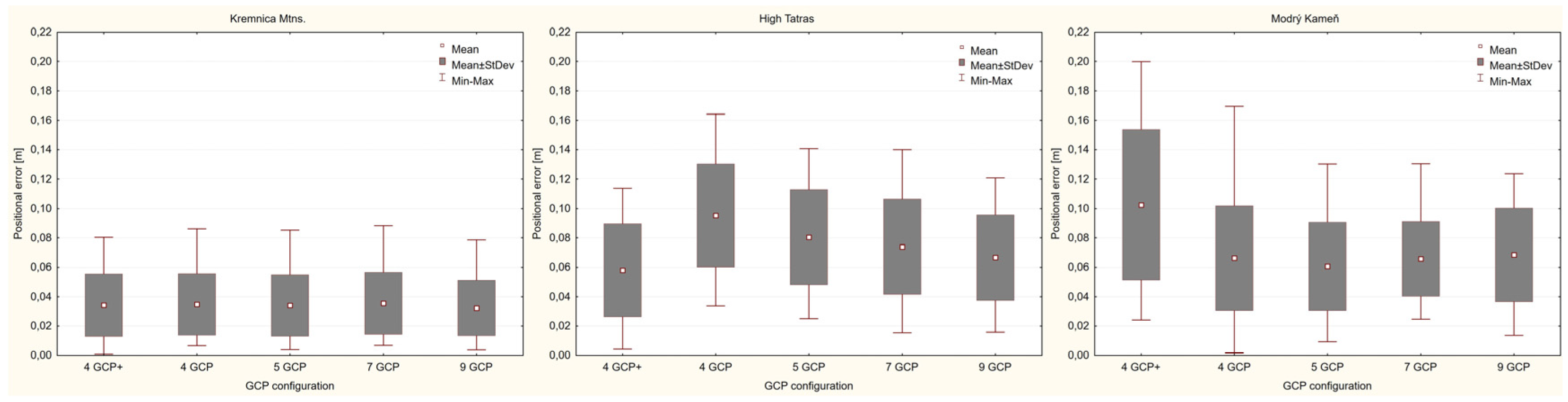
3.1. Horizontal Accuracy

After an initial evaluation, a single point with a positional error of 0.32 m belonging to the “Modrý Kameň” plot was excluded from all subsequent analyses (for both horizontal and vertical accuracy). The horizontal accuracy was evaluated using two measures—the root mean square horizontal error RMSExy (Table 3) and the positional error with related means, minima, maxima, and standard deviations (Figure 4). The RMSExy values varied from 0.037 m to 0.114 m. The evaluation of the significance of between-plot RMSExy differences with the application of the “coefficient of relative efficiency” showed (see Table S1) that the RMSEs of the “Kremnica Mountains” plot were significantly lower compared to both other plots in all tested cases. The RMSExy difference between the “High Tatras” and “Modrý Kameň” plots was significant only for the four-GCP “cross” configuration. The RMSExy differences between the GCP configurations are in the range of 4 mm for the “Kremnica Mountains” plot. For the “High Tatras” site, the RMSExy is decreasing with an increasing number of GCPs (4, 5, 7, 9), but the lowest RMSExy was achieved using the four-GCP “cross” configuration. On the contrary, the RMSExy of the “cross” configuration is the highest for the “Modrý Kameň” plot, while the difference between other configurations is within eight millimetres.
The positional error computed for every checkpoint was used for a more detailed analysis of within-plot variability in groups representing various GCP configurations. The lowest positional error of 0.001 m was achieved at the “Kremnica Mountains” plot, while the highest error of 0.200 m was observed at the “Modrý Kameň” plot. The standard deviations within individual plots are very similar, ranging within a few millimetres. The only exception is the standard deviation for the four-GCP “cross” configuration at the “Modrý Kameň” site, which is visibly higher than the standard deviations of other GCP configurations. The results of the one-way ANOVA with a post-hoc Tukey HSD test (see Supplementary Materials Table S2) did not show any significant difference between the GCP configurations for the “Kremnica Mountains” site. For the “Modrý kameň” site, there is a significant difference between the four-GCP “cross” and the five-GCP configuration. However, the graphic representation in Figure 4 and the p-values of the post-hoc test, which are close to the p < 0.05 criterion, could suggest an important, although not statistically significant, difference between the four-GCP “cross” and all other GCP configurations. The results of the four-GCP “corner” configuration are significantly different—in this case, worse than the four-GCP “cross” and the nine-GCP configurations for the “High Tatras” site.
The spatial distribution of the positional errors acquired on CPs is shown in Figure 5. There is no visible unifying pattern of the error distribution when comparing the test sites. At the Kremnica Mountains site, the distribution of the highest and the lowest errors is random. The highest errors at the “High Tatras” site are concentrated around the north, east, and south edges of the model, while the lowest errors are in the middle and at the west edge. At the “Modrý Kameň” site, the highest errors are concentrated in the northern third and, partially, at the east edge of the model. The lowest errors are in the south half of the model. There is a visible difference in the distribution of the errors between the four-GCP “cross” configuration and all other configuration. The differences between the four-GCP “corner” and the five-, seven-, and nine-GCP configurations are minimal. The spatial pattern remains almost the same, while the values of errors change.

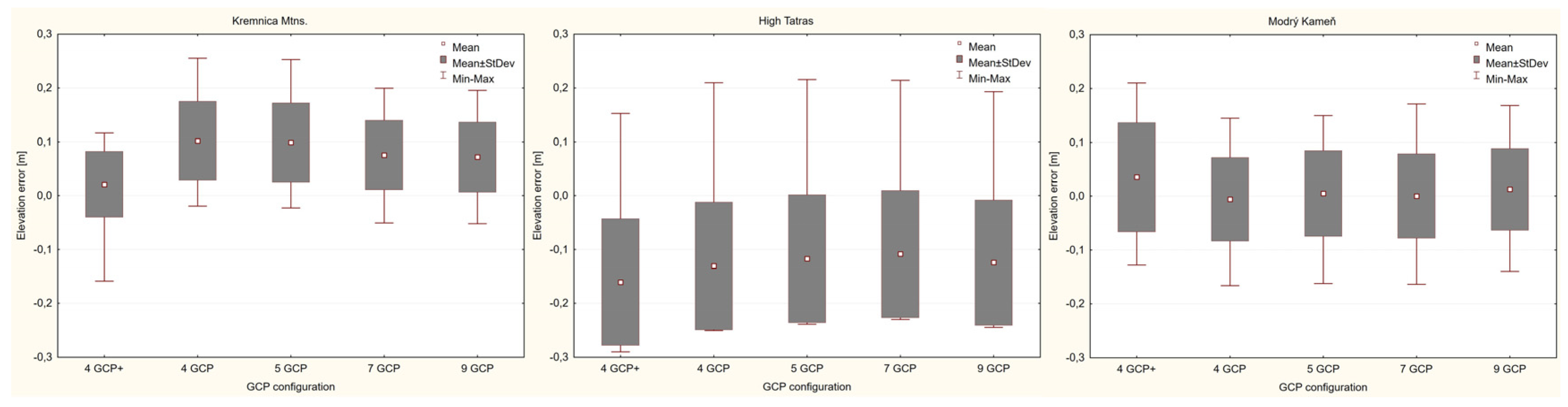
3.2. Vertical Accuracy

The evaluation of the vertical accuracy was based on the root mean square elevation error RMSEz (Table 4) and on the basic statistical characteristics of the observed elevation errors (Figure 6). In contrast to the horizontal accuracy, the lowest RMSEzs can be observed at the “Modrý Kameň” site where to slope was the highest of all test sites. The highest RMSEzs were observed at the moderately-sloped “High Tatras” site, while the RMSEs of the site with the lowest slope—“Kremnica Mountains”—were between the errors of the aforementioned sites. Additionally, the analysis of the RMSEzs showed that RMSEs of the “Modrý Kameň” plot were significantly different from those of the “High Tatras” plot using all GCP configurations. The difference of the “Kremnica Mountains” versus the “High Tatras” and the “Kremnica Mountains” versus “Modrý Kameň” was significant only in some cases.
The occurrence of the highest absolute elevation errors corresponds to the RMSEzs; the highest elevation error of 0.290 m was observed at the “High Tatras” site using the four-GCP “cross” configuration. The successive addition of GCPs (4–5–7–9) had only a slight influence on the range between minimal and maximal errors. The same applies to the standard deviation, where the change was only in a range of millimetres when not considering the four-GCP “cross” configuration. The minimal changes between tested GCP configurations were also confirmed by the one-way ANOVA, where the only significant differences were observed at the “Kremnica Mountains” plot when comparing four-GCP “cross” configuration versus four-GCP “corner” and five-GCP configurations.
The graphic representation of the variance in Figure 6, but also the representation of the spatial distribution of the elevation error suggests an occurrence of bias at the “Kremnica Mountains” and “High Tatras” sites. This bias was also confirmed using the Student’s t-test. The elevation of checkpoints was systematically underestimated at the “High Tatras” plot, while it was systematically overestimated at the “Kremnica Mountains” plot. When considering the spatial distribution of errors, there is no “between-sites” regularity, as there was not any regularity when considering the horizontal errors. The highest errors are concentrated in the left half of the model at the “Kremnica Mountains” site. For “High Tatras”, the highest errors are in the middle and in left corner of the model. In contrast to the horizontal errors, the highest elevation errors of the “Modrý Kameň” are concentrated in the lower half of the model.

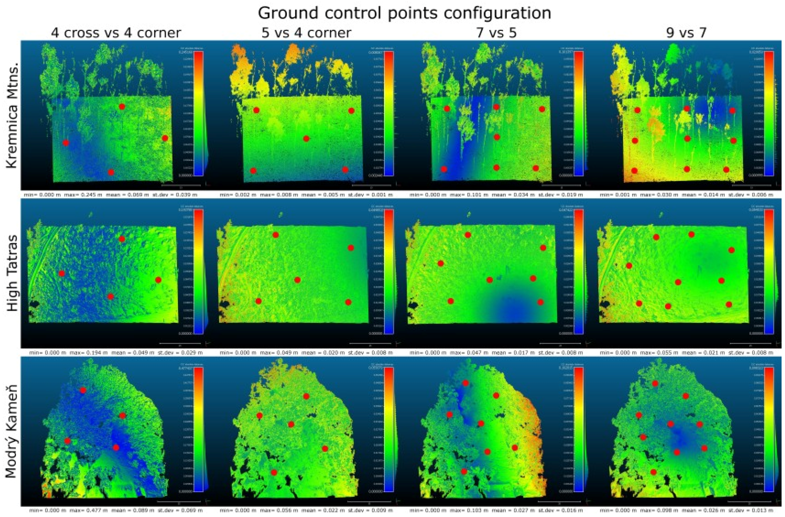
3.3. Overall Changes of Point Clouds

The above-mentioned horizontal and vertical accuracies originate in the manual evaluation of the point-clouds, which inevitably included subjective errors of an operator. Therefore, we also present results of the transformations as reported by the Agisoft Photoscan software (Table 5). The reported errors represent the root mean square transformation residuals at the GCPs. In contrast to the aforementioned horizontal RMSEs, apart from the four-GCP “cross” configuration, the root mean square mean residuals increase with the increasing number of ground control points in most cases. A rapid increase of the root mean square residuals was always related to the addition of a particular point with a high residual value (e.g., four- vs. five-GCP configuration Z-residuals at the Kremnica and High Tatras sites). The reported horizontal RMSEs were, in many cases, lower than the related root mean square residuals. However, the vertical residuals were always lower than the related RMSEs.
The results of a comparison of point-clouds originating in various GCP configurations are presented in Figure 7. Shown are the nearest-neighbour “cloud-to-cloud” distances confirming the results of the horizontal and vertical accuracy analyses in terms of the impact of the GCP configurations. The highest absolute distances were observed when comparing the four-GCP “cross” and four-GCP “corner” configurations—0.245 m for “Kremnica Mountains”, 0.194 m for “High Tatras”, and 0.477 m for “Modrý Kameň” sites. The same applies to the mean absolute distances (0.069 m, 0.049 m and 0.089 m). This supports the conclusions of the accuracy analyses—the majority of significant changes is related to the initial configurations of the GCPs—four “corner” and four “cross”. The changes between the other GCP configurations are lower; the maximal distances range from 0.008 m to 0.102 m, and the means range from 0.005 m to 0.034 m. In several cases, the maximal distances are related to the above-ground vegetation or are not included in the area bordered by GCPs and CPs and, therefore, did not influence the accuracy analyses.

4. Discussion

The horizontal accuracy represented by the root mean square horizontal error RMSExy did not exceed nine centimetres. This root mean square error is a commonly used criterion for the accuracy of mapping. For example, the presented results did not exceed either a cadastral mapping criterion for forested areas or even a stricter criterion required in built-up (residential) areas in Slovakia. The problem here is a relatively small area covered by point clouds, which result from short flight times related to the majority of small UAVs. A higher flight altitude could be a solution here, but this can result in a deterioration of the accuracy related to resolution (ground sample distance) and, in some cases, also in conflict with legal requirements. Therefore, the use of small UAVs is limited in terms of geodetic surveys, where the main tasks are point, line, and area measurements. If precise equipment is needed to determine the positions of GCPs, the same equipment could be used for the mentioned surveys of a small area. Therefore, the main area of small UAV utilisation can be in determining highly-accurate digital elevation models (DEMs) in cases where the small area is not of concern and the required high density of points would be very time-consuming with the application of conventional surveying. The majority of posible applications in forestry is described in the introduction. Studies on the horizontal and vertical accuracy of the SfM-derived model report differing results. Mader et al. [24] reported an RMS value of 0.049 m when comparing SfM-derived points to TLS results during monitoring of a bridge. Hrůza et al. [25] inspected damage of a forest hauling road and reported an altitudinal RMSE of 0.020 m and a positional RMSE of 0.012 m, while the flight altitude was 4–6 m above the surface of the road. Harwin and Lucieer [45] suggest that a point cloud accurate to 25–40 mm can be obtained from imagery acquired from ~50 m flight altitude. Other studies reported RMSEs of residuals of the bundle adjustment transformation on used GCPs as low as a few millimetres [27], or slightly over 1 cm [28], while the flight altitudes were higher—40 m and 120 m. Dandois and Ellis [36] conducted 3D mapping of vegetation dynamics with the use of Ecosynth and UAV imagery. The accuracy was calculated under leaf-on, and also leaf-off, conditions while using six GCPs. The horizontal RMSE varied from 1.21 m to 4.13 m and the vertical RMSE varied from 0.39 m to 1.16 m. In order to reach the terrain in a forest, the canopy must be partially open when using photogrammetry. This is the main limitation when comparing UAV SfM photogrammetry to LIDAR measurements, which are capable of reconstructing surfaces located under trees (e.g., [46,47,48]). Therefore, test plots with a differing degree of tree cover were used in the presented study to enable partial reconstruction of terrain. Such a measurement can be useful, e.g., during the determination of trees or forest stand heights, or various construction tasks in forests, where the precise reconstruction of the terrain is of high priority.
The achieved horizontal accuracy significantly differs between the test plots in most cases. The highest horizontal accuracy was achieved at the Kremnica Mountains plot with RMSEs being significantly lower than the RMSEs at both other test plots. This plot is the smallest one, with minimal slope and minimal changes of micro-relief. The reconstruction of the terrain was highly successful because the imagery was acquired during the leaf-off season. The RMSExy differences at the High Tatras and Modrý Kameň plots were significant only for the four-GCP “cross” configuration. The High Tatras is similar to the Kremnica Mountains plot in terms of slope and open (almost non-existent) canopy, but it is significantly different in terms of micro-relief. After-disturbance conditions at this site are characterised by numerous remaining coarse and fine woody debris and unstable terrain. Even an acquisition of a reliable reference can be problematic under such conditions. The conditions at the Modrý Kameň site are characterised by a higher slope and a sparser occurrence of gaps in the canopy when compared to the other sites. The occurrence of the highest positional errors is concentrated in the highest parts of the site and around the corners of the point cloud. We explain this by lower image overlaps in those parts. This can also be partially applied to the results at the High Tatras site; however, the spatial distribution of the horizontal errors at the Kremnica Mountains site seems to be more random. Additionally, the differing point cloud density could have an influence on the resulting accuracy as the point positions were snapped to the nearest point in the point cloud. Generation of an orthophoto and DEM could be a solution, but this was not the aim of the study. However, the highest horizontal accuracy and the second-highest vertical accuracy was achieved on the test site with the lowest point density. Therefore, we conclude that, in this particular study (and with regard to the achieved ranges of accuracy), the point density did not significantly influence the accuracy. The applied calibration method—precalibration using the Agisoft LENS software—can also be a partial reason for the achieved errors. Although the Photoscan developers recommend this method, Harwin et al. [49] reported that it is inferior to other calibration methods, even to “on-the-job” self-calibration. The differences are within a few millimetres for horizontal accuracy, however, the differences are up to 3.5 cm for the vertical accuracy. Furthermore, a form of GCP and CP signalling can influence the resulting accuracies. A nail representing the exact position of a point was not identifiable in most cases. However, the rectangular shape of signals allowed an experienced operator to use diagonals and other lines to identify the centre. Some photogrammetric software is capable of automatic recognition of GCPs and CPs signalled using coded targets; however, these must be checked and manually refined in most cases.
The resulting measures of the vertical accuracy are higher than those characterising the horizontal accuracy. Surprisingly, the vertical accuracy is the highest at the test site with the highest slope—Modrý Kameň. This site is the only one where there is no evident bias in elevations. Standard deviations at the Kremnica Mountains site are almost the same as at the Modrý Kameň site, but there is evident positive bias in the vertical errors at this site (see Figure 5). Bias is even more evident at the High Tatras site where, in contrast to the others, elevations are systematically underestimated. The standard deviations at this site are also higher than those at the previous sites. This can be explained by the previously described conditions at this site (rugged, unstable terrain). We cannot explain the reasons of the bias occurrence. The first possibility—systematic error in GCPs elevations—was rejected as the elevations of the GCPs and checkpoints were determined during the same survey. Therefore, the checkpoints would be shifted the same way as the GCPs. Another possible explanation is an occurrence of internal transformation error, which we cannot prove. The values of vertical errors resulting from manual evaluation are not in direct relation to the vertical residuals resulting from transformation. In contrast to the horizontal accuracy evaluation, the RMSEzs of the manual evaluation are higher, in some cases equal, when compared to the vertical residuals of the same GCP configurations. Overall, the vertical accuracy of the reconstructed terrain can be suitable for elevation measurements under forest conditions, particularly for tree height measurements. For example, Mikita et al. [2] combined aerial (UAV) and terrestrial photogrammetry point clouds and reported an RMSE value of 1.02 m for tree heights. Wallace et al. [50] reported a tree height RMSE of 1.30 m for MVS-derived point clouds and 0.92 m for LIDAR data acquired using a UAS. Therefore, the vertical errors lower than 0.20 m reported in our study can be considered suitable for this task. The limiting condition is the visibility of terrain as mentioned before. This can only be achieved if there are gaps in the canopy or, in the case of deciduous forest stands, using a combination of point clouds acquired under leaf-on and leaf-off conditions.
One of the main specifics of this study is the determination of the influence of GCP quantity and configuration on the resulting accuracy. There are only a few studies addressing this problem in terms of UAV photogrammetry. Harwin and Lucier [45] used 21, 10, and six ground control points and reported RMSExyz of 3.4 cm, 7.5 cm, and 14.0 cm during coastal monitoring. As the flight altitude and study area extent were similar to those used in our study, the main differences are the applied camera (Canon 550D) and probably to the highest grade, the PMVS2 software used for point cloud generation. In contrast to our study, the count of GCPs had a major impact on accuracy. Agüera-Vega et al. [51] evaluated 4–20 GCPs and acquired optimal results with 15 GCPs on a 17 ha area using a 120 m flight altitude. In contrast to these results, Goldstein et al. [52] evaluated 5–30 GCPs and reported that increasing the number of GCPs beyond 10 does not increase the DSM accuracy. Harwin et al. [49] consider five GCPs a practical minimum, while 13 GCPs as a practical maximum for a 50 m section of a coastal environment photographed from a 15–20 m height. The majority of significant accuracy shifts in our study was related to the four-GCP “cross” configuration in comparison with other differing GCP configurations. However, we did not find any rule—results related to the four-GCP “cross” configuration were better than other GCP configurations in some cases, while worse in others. This applies to the horizontal, as well as the vertical, accuracy. The only significant difference apart from the four-GCP “cross” configuration was the difference between the horizontal errors of four-GCP “corner” and nine-GCP configurations at the High Tatras site. Overall, the addition of ground control points (4, 5, 7, 9) had a minor impact on the resulting accuracy compared with the initial four-GCP configurations (cross vs. corner). However, these results cannot be generalised as the range of included forest conditions is rather small. Further research on the influence of, e.g., area extent, terrain conditions, flight altitude, tree cover, camera calibration, etc., is desirable. The use of four GCPs cannot be recommended from a practical point of view, because any problem with one GCP can make the processing unfeasible. James and Robson [53] suggest that increasing the number of GCPs beyond the technical minimum provides a more robust solution less sensitive to errors on any point. Additionally, the abovementioned authors suggest the use of a higher number of GCPs [51,52]. Tahar [54] tested GCP configurations very similar to those presented in our study and acquired the best results using 8–9 GCPs.
A survey of ground control points in forests is much more complicated than under open-area conditions. The degradation of GNSS signals in forests (e.g., [55,56]) makes it often necessary to use total station measurements. In cases where the survey cannot be conducted from a single occupation point, this means complications and increased time consumption. Therefore, any unfounded increase of the GCP count can negatively affect the effectiveness of the survey. It is preferable to use more precise methods of GCP measurement, e.g., using a tripod-mounted prism instead of a pole-mounted prism, rather than only increasing the number of GCPs. This applies to sites with similar acreage, like those used in this study, and the applied software as well.

5. Conclusions

This study presents the results of terrain point cloud accuracy evaluations under forest conditions with differing degrees of tree cover. As the point clouds were based on images acquired using a UAV, the cover is crucial for the ability to reach the terrain. This is an important difference when comparing point clouds based on photogrammetry and laser scanning. The achieved horizontal accuracy was high in the case that the terrain was successfully reconstructed, reaching sub-decimetre values. Vertical errors lower than 20 cm allow the application of UAV-based point clouds for various tasks related to the vertical structure of a forest, especially the determination of heights of forest stands and individual trees. Furthermore, the quantity of ground control points had only a minor influence on the resulting accuracy in the presented study. The initial configuration of the four basic GCPs had a significant influence in some cases, but without any rule preferring one configuration over another. It can be suggested that in cases of forest sites with similar area (~1 hectare) and with the use of the same software, the quantity of ground control points is only of secondary importance. However, a GCP count near to the technical minimum (3–4) cannot be recommended and the results must be verified under a wider range of conditions. Overall, the accuracy of UAV-based point clouds was high and can be considered reliable for various tasks regarding horizontal and vertical measurements under forest conditions.

Supplementary Materials

The following are available online at www.mdpi.com/1999-4907/8/5/151/s1.

Acknowledgments

This study was supported by the science grant agency of the Ministry of Education, Science, Research, and Sport of the Slovak Republic, and the Slovak Academy of Sciences project VEGA MŠ SR and SAV No. 1/0804/14: “Actualization of mapping, arrangement of forest land ownership and determination of landscape status by modern methods of geodesy and aerial survey”, Slovak Research and Development Agency grant No. APVV-0069-12: “New technology of managing the nature (NEWTON)”, and the Internal Project Agency of the Technical University in Zvolen grant No. 1/2016: “The importance of chestnut orchards in agro-silvo-pastoral systems and health condition assessment of European chestnut using unmanned aerial vehicle”.

Author Contributions

All authors contributed to the initial proposal of methodology; Martin Mokroš conducted the UAV flights and contributed to the writing of the initial manuscript; Šimon Saloň processed the image data; František Chudý, Daniel Tunák, Šimon Saloň and Julián Tomaštík surveyed the reference data; Julián Tomaštík conducted the analyses and wrote the initial draft of the manuscript.

Conflicts of Interest

The authors declare no conflict of interest.

References

  1. Torresan, C.; Berton, A.; Carotenuto, F.; Di, S.F.; Gioli, B.; Matese, A.; Miglietta, F.; Zaldei, A.; Wallace, L. Forestry applications of UAVs in Europe: A review. Int. J. Remote Sens. 2016, 38, 2427–2447. [Google Scholar]
  2. Mikita, T.; Janata, P.; Surový, P. Forest stand inventory based on combined aerial and terrestrial close-range photogrammetry. Forests 2016, 7, 165. [Google Scholar] [CrossRef]
  3. Zhang, J.; Hu, J.; Lian, J.; Fan, Z.; Ouyang, X.; Ye, W. Seeing the forest from drones: Testing the potential of lightweight drones as a tool for long-term forest monitoring. Biol. Conserv. 2016, 198, 60–69. [Google Scholar] [CrossRef]
  4. Guerra-Hernández, J.; González-Ferreiro, E.; Sarmento, A.; Silva, J.; Nunes, A.; Correia, A.C.; Fontes, L.; Tomé, M.; Díaz-Varela, R. Using high resolution UAV imagery to estimate tree variables in Pinus pinea plantation in Portugal. For. Syst. 2016, 25, eSC09. [Google Scholar] [CrossRef]
  5. Puliti, S.; Olerka, H.; Gobakken, T.; Næsset, E. Inventory of Small Forest Areas Using an Unmanned Aerial System. Remote Sens. 2015, 7, 9632–9654. [Google Scholar] [CrossRef]
  6. Wang, C.; Du, H.; Xu, X.; Han, N.; Zhou, G.; Sun, S.; Gao, G. Multi-scale crown closure retrieval for moso bamboo forest using multi-source remotely sensed imagery based on geometric-optical and Erf-BP neural network models. Int. J. Remote Sens. 2015, 36, 5384–5402. [Google Scholar] [CrossRef]
  7. Tuominen, S.; Balazs, A.; Saari, H.; Pölönen, I.; Sarkeala, J.; Viitala, R. Unmanned aerial system imagery and photogrammetric canopy height data in area-based estimation of forest variables. Silva Fenn. 2015, 49, 1348. [Google Scholar] [CrossRef]
  8. Getzin, S.; Nuske, R.S.; Wiegand, K. Using unmanned aerial vehicles (UAV) to quantify spatial gap patterns in forests. Remote Sens. 2014, 6, 6988–7004. [Google Scholar] [CrossRef]
  9. Wallace, L.; Musk, R.; Lucieer, A. An assessment of the repeatability of automatic forest inventory metrics derived from UAV-borne laser scanning data. IEEE Trans. Geosci. Remote Sens. 2014, 52, 7160–7169. [Google Scholar] [CrossRef]
  10. Fritz, A.; Kattenborn, T.; Koch, B. UAV-Based Photogrammetric Point Clouds—Tree Stem Mapping in Open Stands in Comparison to Terrestrial Laser Scanner Point Clouds. Int. Arch. Photogramm. Remote Sens. Spat. Inf. Sci. 2013, XL-1/W2, 141–146. [Google Scholar] [CrossRef]
  11. Jaakkola, A.; Hyyppä, J.; Kukko, A.; Yu, X.; Kaartinen, H.; Lehtomäki, M.; Lin, Y. A low-cost multi-sensoral mobile mapping system and its feasibility for tree measurements. ISPRS J. Photogramm. Remote Sens. 2010, 65, 514–522. [Google Scholar] [CrossRef]
  12. Aicardi, I.; Garbarino, M.; Lingua, A.; Lingua, E.; Marzano, R.; Piras, M. Monitoring Post-Fire Forest Recovery Using Multi-Temporal Digital Surface Models Generated From. EARSeL eProceedings 2016, 15, 1–8. [Google Scholar]
  13. Merino, L.; Caballero, F.; Martínez-De-Dios, J.R.; Maza, I.; Ollero, A. An unmanned aircraft system for automatic forest fire monitoring and measurement. J. Intell. Robot. Syst. Theory Appl. 2012, 65, 533–548. [Google Scholar] [CrossRef]
  14. De Dios, J.R.M.; Merino, L.; Caballero, F.; Ollero, A. Automatic forest-fire measuring using ground stations and unmanned aerial systems. Sensors 2011, 11, 6328–6353. [Google Scholar] [CrossRef] [PubMed]
  15. Lehmann, J.; Nieberding, F.; Prinz, T.; Knoth, C. Analysis of Unmanned Aerial System-Based CIR Images in Forestry—A New Perspective to Monitor Pest Infestation Levels. Forests 2015, 6, 594–612. [Google Scholar] [CrossRef]
  16. Smigaj, M.; Gaulton, R.; Barr, S.L.; Suárez, J.C. Uav-Borne Thermal Imaging for Forest Health Monitoring: Detection of Disease-Induced Canopy Temperature Increase. ISPRS Int. Arch. Photogramm. Remote Sens. Spat. Inf. Sci. 2015, XL-3/W3, 349–354. [Google Scholar] [CrossRef]
  17. Näsi, R.; Honkavaara, E.; Lyytikäinen-Saarenmaa, P.; Blomqvist, M.; Litkey, P.; Hakala, T.; Viljanen, N.; Kantola, T.; Tanhuanpää, T.; Holopainen, M. Using UAV-Based Photogrammetry and Hyperspectral Imaging for Mapping Bark Beetle Damage at Tree-Level. Remote Sens. 2015, 7, 15467–15493. [Google Scholar] [CrossRef]
  18. Lisein, J.; Michez, A.; Claessens, H.; Lejeune, P. Discrimination of Deciduous Tree Species from Time Series of Unmanned Aerial System Imagery. PLoS ONE 2015, 10, e0141006. [Google Scholar] [CrossRef] [PubMed]
  19. Wallace, L.; Lucieer, A.; Watson, C.S. Evaluating tree detection and segmentation routines on very high resolution UAV LiDAR ata. IEEE Trans. Geosci. Remote Sens. 2014, 52, 7619–7628. [Google Scholar] [CrossRef]
  20. Gini, R.; Passoni, D.; Pinto, L.; Sona, G. Use of unmanned aerial systems for multispectral survey and tree classification: A test in a park area of northern Italy. Eur. J. Remote Sens. 2014, 47, 251–269. [Google Scholar] [CrossRef]
  21. Pierzchała, M.; Talbot, B.; Astrup, R. Estimating soil displacement from timber extraction trails in steep terrain: Application of an unmanned aircraft for 3D modelling. Forests 2014, 5, 1212–1223. [Google Scholar] [CrossRef]
  22. Gómez-Candón, D.; De Castro, A.I.; López-Granados, F. Assessing the accuracy of mosaics from unmanned aerial vehicle (UAV) imagery for precision agriculture purposes in wheat. Precis. Agric. 2014, 15, 44–56. [Google Scholar] [CrossRef]
  23. Xiang, H.; Tian, L. Development of a low-cost agricultural remote sensing system based on an autonomous unmanned aerial vehicle (UAV). Biosyst. Eng. 2011, 108, 174–190. [Google Scholar] [CrossRef]
  24. Mader, D.; Blaskow, R.; Westfeld, P.; Maas, H.G. UAV-Based acquisition of 3D point cloud—A comparison of a low-cost laser scanner and SFM-tools. Int. Arch. Photogramm. Remote Sens. Spat. Inf. Sci. 2015, 40, 335–341. [Google Scholar] [CrossRef]
  25. Hrůza, P.; Mikita, T.; Janata, P. Monitoring of forest hauling roads wearing course damage using unmanned aerial systems. Acta Univ. Agric. Silvic. Mendel. Brun. 2016, 64, 1537–1546. [Google Scholar] [CrossRef]
  26. Ruggles, S.; Clark, J.; Franke, K.W.; Wolfe, D.; Reimschiissel, B.; Martin, R.A.; Okeson, T.J.; Hedengren, J.D. Comparison of SfM Computer Vision Point Clouds of a Landslide Derived from Multiple Small UAV Platforms and Sensors to a TLS based Model. J. Unmanned Veh. Syst. 2016, 4, 246–265. [Google Scholar] [CrossRef]
  27. Mancini, F.; Dubbini, M.; Gattelli, M.; Stecchi, F.; Fabbri, S.; Gabbianelli, G. Using Unmanned Aerial Vehicles (UAV) for High-Resolution Reconstruction of Topography: The Structure from Motion Approach on Coastal Environments. Remote Sens. 2013, 5, 6880–6898. [Google Scholar] [CrossRef]
  28. Boon, M.A.; Greenfield, R.; Tesfamichael, S. Unmanned Aerial Vehicle (UAV) Photogrammetry Produces Accurate High-Resolution Orthophotos, Point Clouds and Surface Models for Mapping Wetlands. S. Afr. J. Geomat. 2016, 5, 186–200. [Google Scholar] [CrossRef]
  29. Sauerbier, M.; Eisenbeiss, H. Uavs for the Documentation of Archaeological Excavations. Int. Arch. Photogramm. Remote Sens. Spat. Inf. Sci. 2010, 38, 526–531. [Google Scholar]
  30. Bird, D.M. Unmanned Vehicle Systems and Wildlife Management in the 21st Century. Presentation. 2014. Available online: https://www.exeter.ac.uk/media/universityofexeter/esi/documents/uavmeetingpapers/D._Bird,_RSPB,_July_2014.pdf (accessed on 10 October 2016).
  31. Laliberte, A.S.; Herrick, J.E.; Rango, A.; Winters, C. Acquisition, Orthorectification, and Object-based Classification of Unmanned Aerial Vehicle (UAV) Imagery for Rangeland Monitoring. Photogramm. Eng. Remote Sens. 2010, 76, 661–672. [Google Scholar] [CrossRef]
  32. Nex, F.; Remondino, F. UAV for 3D mapping applications: A review. Appl. Geomat. 2014, 6, 1–15. [Google Scholar] [CrossRef]
  33. Hůlek, D.; Němec, V.; Szabo, S.; Sodomka, J. Current State of the Small RPAS Maintenance in the Czech Republic. Perner’s Contacts 2016, 11, 25–30. [Google Scholar]
  34. Westoby, M.J.; Brasington, J.; Glasser, N.F.; Hambrey, M.J.; Reynolds, J.M. “Structure-from-Motion” photogrammetry: A low-cost, effective tool for geoscience applications. Geomorphology 2012, 179, 300–314. [Google Scholar] [CrossRef]
  35. Erenoglu, R.C. Generating a Digital Elevation Model using Unmanned Aerial System. Austrian J. For. Sci. 2016, 133, 47–61. [Google Scholar]
  36. Dandois, J.P.; Ellis, E.C. High spatial resolution three-dimensional mapping of vegetation spectral dynamics using computer vision. Remote Sens. Environ. 2013, 136, 259–276. [Google Scholar] [CrossRef]
  37. Dunford, R.; Michel, K.; Gagnage, M.; Piégay, H.; Trémelo, M.-L. Potential and constraints of Unmanned Aerial Vehicle technology for the characterization of Mediterranean riparian forest. Int. J. Remote Sens. 2009, 30, 4915–4935. [Google Scholar] [CrossRef]
  38. Haala, N.; Cramer, M.; Rothermel, M. Quality of 3D Point Clouds from Highly Overlapping UAV Imagery. Int. Arch. Photogramm. Remote Sens. Spat. Inf. Sci. 2013, XL-1/W2, 4–6. [Google Scholar] [CrossRef]
  39. Tahar, K.; Ahmad, A. An Evaluation on Fixed Wing and Multi-Rotor UAV Images using Photogrammetric Image Processing. Waset Org. 2013, 73, 391–396. [Google Scholar]
  40. AgiSoft PhotoScan Professional. Software. Version 1.2.6. 2016. Available online: http://www.agisoft.com/downloads/installer/ (accessed on 10 October 2016).
  41. Šmelko, Š. Dendrometry; Technical University in Zvolen: Zvolen, Slovakia, 2007; p. 400. [Google Scholar]
  42. StatSoft, Inc. STATISTICA (Data Analysis Software System). Version 10. 2011. Available online: www.statsoft.com (accessed on 10 October 2016).
  43. QGIS Development Team. QGIS Geographic Information System. Open Source Geospatial Foundation Project. 2016. Available online: http://www.qgis.org/ (accessed on 10 October 2016).
  44. CloudCompare. GPL Software. Version 2.9 Alpha. 2016. Available online: http://www.cloudcompare.org/ (accessed on 10 October 2016).
  45. Harwin, S.; Lucieer, A. Assessing the accuracy of georeferenced point clouds produced via multi-view stereopsis from Unmanned Aerial Vehicle (UAV) imagery. Remote Sens. 2012, 4, 1573–1599. [Google Scholar] [CrossRef]
  46. James, L.A.; Watson, D.G.; Hansen, W.F. Using LiDAR data to map gullies and headwater streams under forest canopy: South Carolina, USA. Catena 2007, 71, 132–144. [Google Scholar] [CrossRef]
  47. Chisholm, R.A.; Cui, J.; Lum, S.K.Y.; Chen, B.M. UAV LiDAR for below-canopy forest surveys. J. Unmanned Veh. Syst. 2013, 1, 61–68. [Google Scholar] [CrossRef]
  48. Smreček, R.; Danihelová, Z. Forest stand height determination from low point density airborne laser scanning data in Rožňava Forest enterprise zone (Slovakia). IForest 2013, 6, 48–54. [Google Scholar] [CrossRef]
  49. Harwin, S.; Lucieer, A.; Osborn, J. The impact of the calibration method on the accuracy of point clouds derived using unmanned aerial vehicle multi-view stereopsis. Remote Sens. 2015, 7, 11933–11953. [Google Scholar] [CrossRef]
  50. Wallace, L.; Lucieer, A.; Malenovskỳ, Z.; Turner, D.; Vopěnka, P. Assessment of forest structure using two UAV techniques: A comparison of airborne laser scanning and structure from motion (SfM) point clouds. Forests 2016, 7, 62. [Google Scholar] [CrossRef]
  51. Agüera-Vega, F.; Carvajal-Ramírez, F.; Martínez-Carricondo, P. Assessment of photogrammetric mapping accuracy based on variation ground control points number using unmanned aerial vehicle. Measurement 2017, 98, 221–227. [Google Scholar] [CrossRef]
  52. Goldstein, E.B.; Oliver, A.R.; DeVries, E.; Moore, L.J.; Jass, T. Ground control point requirements for structure-from-motion derived topography in low-slope coastal environments. PeerJ 2015. [Google Scholar] [CrossRef]
  53. James, M.R.; Robson, S. Straightforward reconstruction of 3D surfaces and topography with a camera: Accuracy and geoscience application. J. Geophys. Res. Earth Surf. 2012, 117, F03107. [Google Scholar] [CrossRef]
  54. Tahar, K.N. An evaluation of different number of ground control points in unmanned aerial vehicle photogrammetric block. Int. Arch. Photogramm. Remote Sens. Spat. Inf. Sci. 2013, XL-2/W2, 27–29. [Google Scholar] [CrossRef]
  55. Trajkovski, K.K.; Sterle, O.; Stopar, B. Sturdy positioning with high sensitivity GPS sensors under adverse conditions. Sensors 2010, 10, 8332–8347. [Google Scholar] [CrossRef] [PubMed]
  56. Ucar, Z.; Bettinger, P.; Weaver, S.; Merry, K.L.; Faw, K. Dynamic accuracy of recreation-grade GPS receivers in oak-hickory forests. Forestry 2014, 87, 504–511. [Google Scholar] [CrossRef]
Figure 1. Location of the test plots.
Forests 08 00151 g001
Figure 2. Ground control point and checkpoint: (a) photo; and (b) point cloud.
Forests 08 00151 g002
Figure 3. Ground control points (GCPs) and checkpoints. (a) The design of the GCP configurations (4: four-GCP “corner”; 4+: four-GCP “cross”; 5: fifth point in the middle; 7: two more points in the slope direction; 9: two more points in the direction of the contour lines). Actual distribution of ground control points and checkpoints on the Kremnica Mountains; (b) High Tatras (c); and Modrý Kameň (d) sites.
Forests 08 00151 g003
Figure 4. Minima, maxima, means and standard deviations of the positional errors Δp according to the test sites and GCP configurations.
Forests 08 00151 g004
Figure 5. Spatial distribution of horizontal and vertical errors according to test site and GCP configuration. Only errors at the checkpoints (marked) were used for the interpolation.
Forests 08 00151 g005
Figure 6. Minima, maxima, means, and standard deviations of the elevation errors Δz according to the test sites and GCP configurations.
Forests 08 00151 g006
Figure 7. Cloud-to-cloud absolute distances between point clouds resulting from differing GCP configurations according to test sites. GCPs are marked with red dots.
Forests 08 00151 g007
Table 1. Test plots characteristics.
Test SiteTree Cover 1Dominant Tree SpeciesAgeHeight (m)Slope (mean ± SD)Vegetation PeriodAMSL 2 (m)
Kremnica Mountains18%Fagus sylvatica65217 ± 2%Non623–626
High Tatras7%Larix decidua752613 ± 5%Veg.1217–1224
Modrý Kameň63%Castanea sativa6–1001839 ± 14%Veg.355–377
1 Orthogonal projection of trees (foliage, branches, stems); 2 elevation above mean sea level.
Table 2. Flight and point-cloud parameters according to the test sites.
Test SiteFlight ParametersPoint-Cloud Parameters
No. of PhotosNo. of StripsNo. of Flights 1Flight Duration 1AreaNumber of PointsAverage Points/m2
Kremnica Mountains2414225 min46 m × 44 m1,904,395941
High Tatras1616218 min71 m × 92 m9,659,1761479
Modrý Kameň3335328 min103 m × 113 m33,841,2982908
1 Including preliminary flight needed for trajectory planning.
Table 3. Root mean square horizontal errors RMSExy according to the test sites and GCP configurations (in metres).
Test SiteGCP Configuration
4+4579
Kremnica Mountains0.0400.0400.0400.0410.037
High Tatras0.0660.1010.0860.0800.072
Modrý Kameň0.1140.0750.0670.0700.075
Table 4. Root mean square elevation errors RMSEz according to the test sites and GCP configurations (in metres).
Test SiteGCP Configuration
4+4579
Kremnica Mountains0.0640.1250.1220.0980.096
High Tatras0.1980.1750.1650.1580.169
Modrý Kameň0.1060.0770.0780.0770.076
Table 5. Root mean square horizontal and vertical residuals at the ground control points after transformation.
Test SiteErrorGCP Configuration
4+4579
Kremnica MtnsXY0.0310.0220.0210.0330.031
Z0.0490.0180.0530.0450.058
High TatrasXY0.0430.0910.0890.0800.079
Z0.0840.0160.0780.0690.076
Modrý KameňXY0.0490.0610.0740.0720.075
Z0.0570.0230.0300.0600.062

