
Tree Species Site Suitability as a Combination of Occurrence Probability and Growth and Derivation of Priority Regions for Climate Change Adaptation

Institute of Geography and Geoecology—Karlsruhe Institute of Technology (KIT), Kaiserstr. 12, 76131 Karlsruhe, Germany
*
Author to whom correspondence should be addressed.
Forests 2017, 8(6), 181; https://doi.org/10.3390/f8060181
Submission received: 15 February 2017
/
Revised: 8 May 2017
/
Accepted: 17 May 2017
/
Published: 24 May 2017
(This article belongs to the Special Issue Impacts of Climate Change—Selected Papers from FowiTa German Forest Sciences Conference (Sessions 1–5))
Abstract
:Two aspects of site suitability were combined, namely species occurrence probability and tree growth as proxies for risk and productivity, aiming to improve climate impact assessments for forests. This measure was used to identify priority regions for climate change adaptation under consideration of current stands. The six most frequent tree species according to German national forest inventory data were used considering repeated measurements. Species distribution and growth models were calculated and combined into one measure. To identify priority regions regarding current forests, we aggregated species-specific negative development of site suitability for stands where a tree species actually occurred. Suitability under climate change increased or remained unchanged for current stands of silver fir, pedunculate oak and sessile oak. European beech and Scots pine showed large area shares with negative changes, but also areas with positive changes in site suitability. For Norway spruce, suitability decreased strongly. Priority regions were concentrated in the federal states Rhineland-Palatinate, Hesse, Baden-Württemberg, Thuringia, Lower Saxony, and Saxony-Anhalt. Certainly, the workflow contained several steps, at which decisions had to be made. Although this work did not resolve all issues of site suitability modeling for climate impact on forests, it provided a more comprehensive view on tree species site suitability in biogeographical modeling.
1. Introduction
Although Central European forests have great natural adaptive capacity, management support will be needed to adapt to climate change without economic loss [1]. For some forest stands, climate change will affect stability and timber yield negatively. Ideally, economically-oriented management measures reduce risk, increase stability and thereby optimize yield. In Germany, considerable resources for climate change adaptation are available but not enough for forest conversion throughout the whole territory. It is not possible to protect all managed forest from negative climate change impact due to constraints in time and costs. To keep losses as low as possible, one strategy is to concentrate efforts on the most vulnerable areas. Scientific methods are thus needed to identify priority regions for climate change adaptation depending on the information available for the forested area of Germany.
A frequently used proxy for climate change impact on forests is change in site suitability. (Here, we use the term as it is used in macroecology, which is not a direct translation of the technical term `Standorteignung’ used in German forestry. Species distribution models (SDMs) and growth models are macroecological approaches and apply to a coarser scale than site suitability mapping in forestry usually does.) In climate impact research, the outcome of SDMs and derivatives of occurrence probability are often interpreted as site suitability [2,3]. However, productivity of trees is ignored when this method is used for assessing site suitability. Information about how well a tree species grows on a certain site is important to forest managers. Another issue with SDMs for managed species is that models will provide site suitability estimates based on the actual distribution and it is impossible to derive estimates for the natural or even potential distribution [4,5,6], which would perhaps be more useful as a basis for decisions on climate change adaptation. Nevertheless, SDMs contain information about one aspect of site suitability: whether a species can at least tolerate the conditions at a site where it occurs. Because of the inherent limitations of SDMs, Guisan and Thuiller (2005) [5] suggested additionally considering community ecology, demographic processes, and biotic interactions.
The distribution of species is indeed a result of different demographic processes which in turn are influenced by abiotic as well as biotic interactions such as competition [7,8]. Growth is one of the processes which determine species distribution. Growth parameters are also used to estimate species’ ecological demands and responses to climate change [9,10,11,12,13,14]. When competition is considered, tree growth can be assumed to be less influenced by human management than distribution, which is an advantage for determining site suitability. Besides from being less influenced by management, tree and stand growth are also important measures for site productivity.
In recent years, estimates for climatic site suitability focused on risk which is reflected by occurrence probabilities calculated from species distribution [15,16,17,18]. The German national forest inventory (NFI) provided a solid data basis for the calculation of such SDMs [19]. Until now, few studies have compared multiple aspects of site suitability to obtain a more comprehensive picture, e.g., Albrecht et al. (2015) [20] combined two aspects—risk and productivity—by coupling a tree growth model with a storm damage model. Assessments of site suitability in the context of climate change on the basis of species distribution on the one hand and growth on the other hand can lead to contradictory results [21,22]. This shows the disparate information contents and, thus, the importance of considering several properties. Dolos et al. (2015) [22] found discrepancies in modeled tree species’ growth and distribution. In order to consider both—information in species distribution and tree growth—we combined these two attributes into one index of site suitability. The combination of both information sources for site suitability modeling is a step forwards in climate impact modeling in the forest sector.
Spatial projections for species distribution and tree growth provide information on current and future site suitability. Climate change impact assessments often use continuous maps of changes in site suitability to evaluate the potential of species under climate change. However, to assess the severity of climate change impact, a crucial question is what will happen to current forested areas. Which current stands with a certain species composition need to be actively adapted by management measures and which stands will be less affected due to an already suitable species composition? In forest management, information on regions for which strong negative changes can be expected—i.e., vulnerable areas—helps to concentrate resources. On the basis of maps for current and future site suitability, regions can be identified which are expected to show strong negative changes in the next decades [15,16,18]. In consideration of forested area and its current tree species composition and how site suitability for important tree species is likely to change, priority regions for adaptive management can be identified.
In this study, we (1) developed valid SDMs and growth models based on the German national forest inventories for six tree species; (2) suggested a method to combine these two aspects of site suitability into one measure; and (3) identified priority regions for climate change adaptation of forests under consideration of actual current stands.
2. Materials and Methods
2.1. National Forest Inventory Data
The German national forest inventories (NFI) provided information about forest trees from three repetitions. This database is a valuable tool for studying forest dynamics [19]. Primarily, NFI data are used for assessing growing stock and the value of forest stands, but ecological processes, forest state and stability can also be estimated with NFI data. Between 1986 and 1989, the first inventory was conducted in the Old Federal States, the second between 2000 and 2002 for the whole of Germany and the third between 2011 and 2014. The German NFI design follows a regular grid with a 4 km grid point distance. Some federal states use a denser grid (2 km). Each grid point consists of up to four NFI plots which are at a distance of 150 m from each other. We used stand information based on angle count sampling—also known as Bitterlich sampling—with basal area factor 4 m2/ha (for further details, see [19]). Only trees with a diameter at breast height (DBH) of at least 7 cm were recorded. The youngest trees were five years old and the oldest around 700 years (based on estimations; median: 69 years).
Species information about the six most frequent forest tree species (Table A1) was considered—these six species are also the most important species for German forestry. They were Norway spruce (Picea abies), European beech (Fagus sylvatica), silver fir (Abies alba), Scots pine (Pinus sylvestris), sessile oak (Quercus petraea), and pedunculate oak (Quercus robur). Occurrences of silver fir around the northern regions (n = 34) were excluded from the dataset because its reported natural distribution is limited to the southern part of Germany [23,24]. It is unclear to which provenance planted occurrences further north belong to, particularly bearing in mind that silver fir even has a mountainous Mediterranean ecotype [25]. We excluded negative and zero growth as this was presumably attributed to measurement errors.
We used species, position and DBH from three repetitions (reference years: 1987, 2002, and 2012). We calculated the annual relative basal area increment (relBAI; Equations (1) and (2)) which was used as a response variable in the growth models.
- : Basal area of a single tree at time t
- : Diameter at breast height at time t
- : Annual relative basal area increment
- : Basal area of a single tree at time t
- : Measuring time (here: NFI 1, NFI 2)
- : Exact time interval in days between the measurement dates divided by 365.25
Additionally, slope-corrected stand basal area (SBA) was calculated and used as an explanatory variable in the growth model to account for light availability and competition (Equations (3) and (4)).
- c: Slope correction factor
- : Slope
- : Stand basal area
- N: Number of trees of an inventory plot
- k: Basal area factor
- c: Slope correction factor
We also calculated stand basal area of larger trees. The population of all larger individual trees was calculated individually for each tree [26]. Stand basal area of larger trees is the sum of the basal areas of all trees of a plot which have a larger DBH than the target tree. For this reason, for the smallest individual, it is equal to the stand basal area and zero for the largest individual. Surprisingly, in the variable selection it dropped, because stand basal area was as good as or even better than basal area of larger trees.
SDMs were calculated for the second and third NFI only, because Germany’s Old Federal States were not included in the first NFI. Both periods were used for the growth models.
2.2. Environmental Data
Climatic variables were calculated using data from the German weather service (DWD). Mean annual temperature and annual precipitation were provided in 1 × 1 km2 rasters. Additionally, we calculated 19 BioClim variables with the R package dismo [27].
For SDMs, we chose a long-term average of thirty years for climatic variables. Thirty years is a meteorological standard to characterize climate. This time period also likely covered the time span important for current stands. Moreover, no climate data in sufficient quality were available prior to 1961. Additionally, we assumed that the climatic impact on species distribution during the last ten years was less important for the presence of tree species because of the delayed response of living organisms to the climate. Considering those factors, the resulting time spans were 1961–1990 for NFI 2 and 1984–2002 for NFI 3.
For growth models, we chose the time period between 1984 and 2002 for climatic variables for the period between the first (1986–1989) and the second NFI (2000–2002). Two years prior to the beginning of the growth period were added, because it was found that tree growth reactions to climatic conditions are delayed [28]. Accordingly, for the second growth period between the second and the third NFI (2011–2014), we chose the time period between 1998 and 2014.
For climate change projections, a regionalized RCP 8.5 [29] scenario was used, which was an ensemble of eight members [30,31]. The ensemble median was used for all following calculations. For SDM projections, thirty-year means (2021–2050), and for growth model projections, ten-year means (2041–2050) were used. The resolution was 7 × 7 km2, thus differed from the dataset used for model fitting (which was 1 × 1 km2). We decided to remain with the higher resolution of the DWD climate data to derive the best models for current climatic conditions. Resolution of raster files for the climate change scenario was increased to 1 × 1 km2 to match the resolution of DWD rasters. This increase in resolution was only a necessary step in data handling since we combined rasters, and did not increase the spatial information on the climate. These differences in spatial resolution between data used in model fitting and data used for climate change projections caused the distribution of climatic variables and subsequently model projections to be less extreme because extremes are underestimated in coarser rasters. High as well as low projected values for occurrence probability and growth were attenuated and this needs to be considered in interpretations.
Soil data were taken from the European soil database. Originally, 72 soil types were accumulated to 12 main soil types [32].
2.3. Species Distribution Models
For the selected six species, species distribution models were calculated using generalized additive models (GAM) using thin plate regression splines [33] with a binomial error distribution. The target variable for the SDM was the presence or absence of a tree species. Species occurrence was explained by temperature, precipitation and soil type. An interaction term for temperature and precipitation was included by using a two-dimensional spline. All explanatory variables were scaled. The models followed the structure below (Equation (5)):
- p: Occurrence of a tree species (presence, absence; binary)
- T: Mean annual temperature or other temperature-related BioClim variable
- P: Mean annual precipitation sum or other precipitation-related BioClim variable
- S: Soil type (factor with 12 levels)
- i: Index of summation
- : Parameters
- : Thin plate splines with basis dimension k = 3
- : Thin plate spline for interaction with basis dimension k = 5
- : Error (binomial distribution)
First, we assessed the difference among models for the second and third NFI. There were only very little differences in the data of the second and the third NFI and, therefore, in the models. Hence, we remained with the third NFI only in order to save computation time.
The number of NFI plots at each grid point ranged from 1 to 4 depending on whether the area was forested or not. Each plot was intended to make the same contribution to the model. Therefore, the total weight of each plot belonging to the same grid point was divided by the number of plots at the respective grid point. Accordingly, these weights ranged between 1 (one forested plot per grid point) and 0.25 (four forested plots).
An exhaustive search for the best variables was performed. The Akaike information criterion (AIC) [34] and explained deviance were used to identify the best models. We tested all possible combinations of variables, each combination resulting in a model not exceeding one temperature-related and one precipitation-related BioClim variable.
Repeated data splitting was applied with a share of 70% training and 30% test data with 100 repetitions.
2.4. Growth Models
For growth modeling, we used a GAM with annual relative basal area increment (relBAI) as a response variable and a log-link function with gamma distributed error. Explanatory variables were temperature, precipitation, soil type, SBA, and DBH. We used the following formula (Equation (6)):
- : Annual relative basal area increment
- T: Mean annual temperature or other temperature-related BioClim variable
- P: Mean annual precipitation sum or other precipitation-related BioClim variable
- S: Soil type (factor with 12 levels)
- i: Index of summation
- : Diameter at breast height
- : Stand basal area (or stand basal area of larger trees)
- : Parameters
- : Thin plate splines with basis dimension k = 3
- : Thin plate spline for interaction with basis dimension k = 5
- : Error (binomial distribution)
Because growth as well as climate differed in periods NFI 1/2 and NFI 2/3, it was reasonable to use both time steps in one model. The challenge of using multiple time steps in one model is correlation among samples—in our study, there were two observations per individual tree. For such a case, mixed effect models would be suitable. In this study, however, there was a huge amount of statistical units (individual trees) with few measurements (NFI time steps). Therefore, computation resources were not enough to fit these models. Hence, instead of mixed effect models, we used marginal models as the second best choice [38]. The correlation matrices with the grouping factor `individual tree’ allowed us to use two measurements per individual tree, taking temporal autocorrelation into account. We did not use this method for both oak species, because they were not recorded separately in the first NFI. Thus, for oaks, normal GAMs and growth between NFI 2 and 3 were fitted.
Additionally, in the growth model, weights were used to account for the sampling design. Weights were calculated the same way as for SDMs. These plot weights were then divided by the number of trees at the respective plot.
Variable selection was done analogously to the procedure for SDMs.
2.5. Combining Distribution and Growth
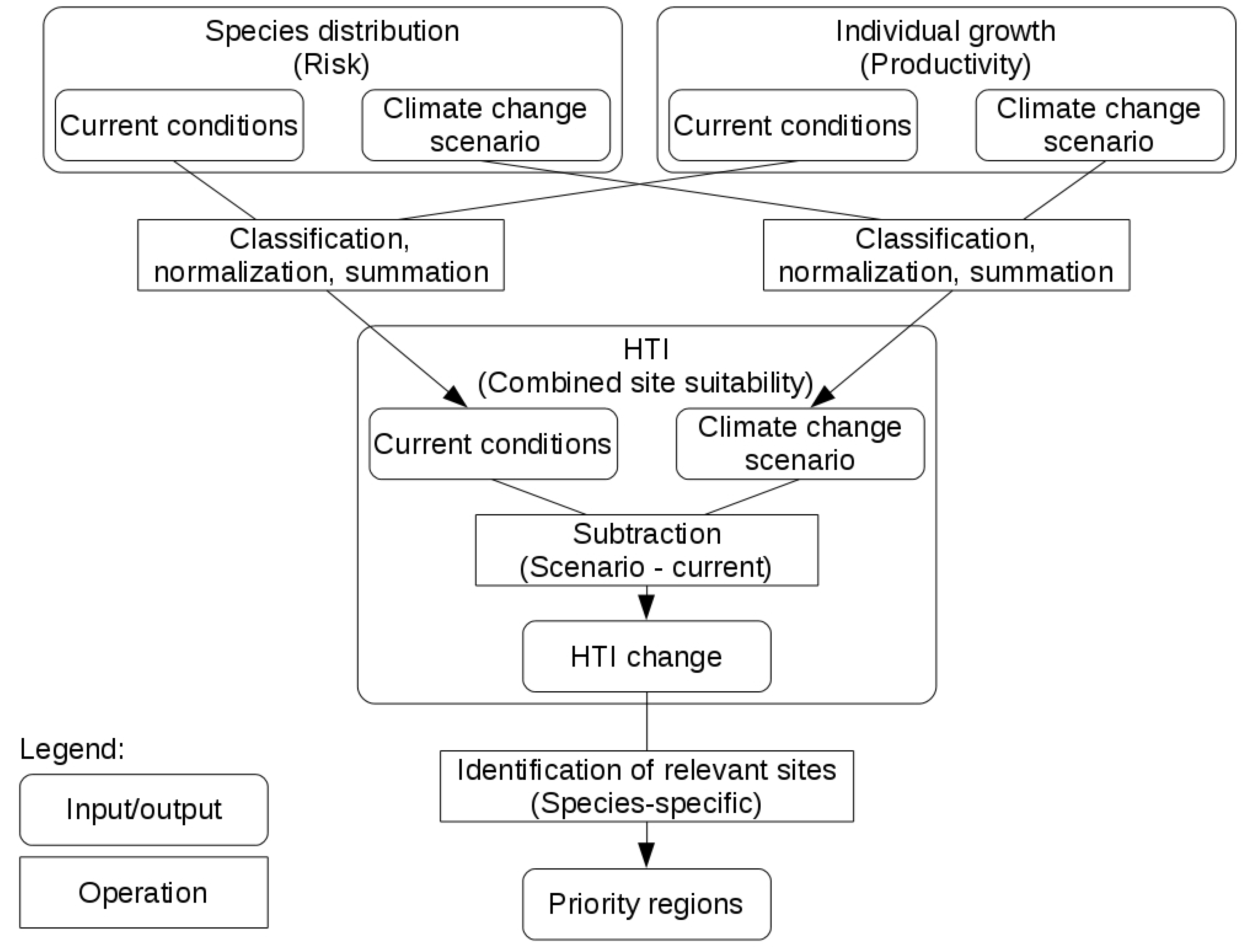
Predictions for occurrence probability and tree growth were combined in order to reduce complexity and allow the identification of regions with strong expected negative change of site suitability under climate change, i.e., priority regions. This was done in several steps (Figure 1). After model fitting, predictions for the current climate were calculated for NFI sites (point data). Analogously to Hanewinkel et al. (2014) [18], we calculated ecologically meaningful thresholds for occurrence probability (TV1, TV2, TV3). To obtain finer gradations, two additional thresholds (TV1a, TV3a) were added (Table A2). Thresholds for SDMs were calculated for each species based on fitted values for all NFI sites under current climate.
For growth, the same number of classes as for species distribution was chosen. We derived five thresholds from quantiles of the predictions at NFI plots where the species was present (quantiles = 1/6, 2/6, ... , 5/6). Because SBA and DBH were not available for the whole area but only at NFI sites, we used the medians of these two variables for spatial projections and, therefore, for deriving the thresholds as well.
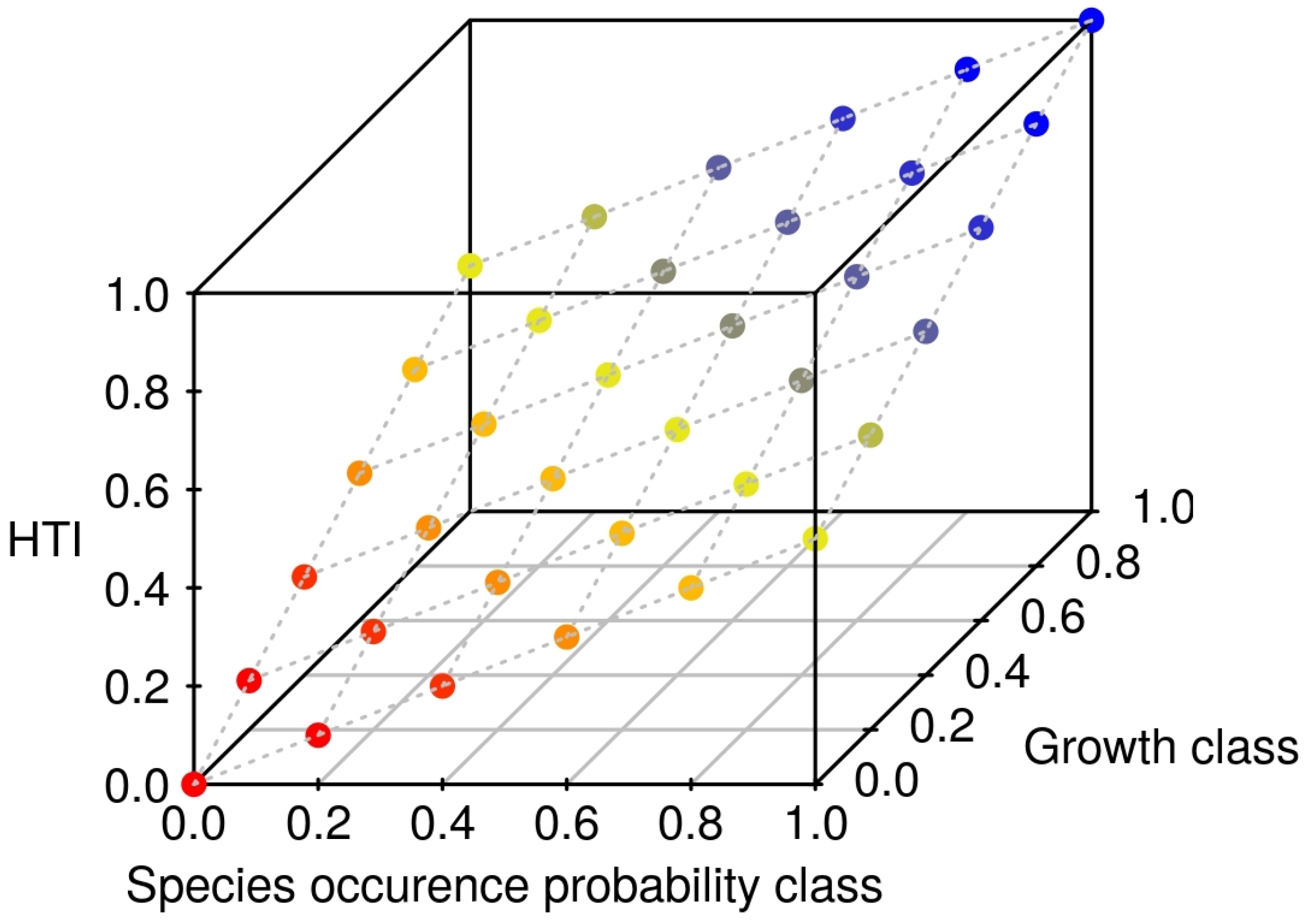
Class values 1–6 were each normalized to 1 by dividing by the number of classes. By this procedure, the two different variable types were transformed to values between 0 and 1, i.e., were standardized to the same range. Lastly, their sum was formed to obtain the happy tree index (HTI) for each pixel (Equation (7), Figure 1 and Figure A1).
By calculating the sum, occurrence probability and tree growth were implicitly weighted 1:1—bearing in mind that calculating class thresholds as well as a direct combination already influenced weighting. The HTI was kept in the range between 0 and 1 by dividing by the number of summands.
SDMs and growth models were applied to two different datasets—one with main soil types and current climate conditions and one with main soil types and the climate change scenario [30,31]. These maps were used to derive an HTI map for each species under the current climate and the climate change scenario (Equation (7), Figure 1). Values were projected for the whole of Germany. Thus, spatial projections of site suitability needed to be interpreted carefully because of constraints in habitat availability.
The resulting species distribution, growth, and HTI maps for the current climate and the climate change scenario were masked with forested area (Coordinated Information on the European Environment (CORINE) land cover data [39]). The maps were displayed without masking and in the appendix with the forest mask applied. The forest mask was applied to evaluate site suitability and its changes considering area actually available for forestry. We assumed that the extent of forested area would not change considerably during the next decades [40].
2.6. HTI Changes
Differences in HTI under current and climate change scenario conditions were calculated for each species. Since this study aimed to identify areas for which adaptation of stands is needed under consideration of current stands, areas in which the species actually occurred with a relevant density were identified. All NFI sites with a basal area share of the target species larger than the 75% quantile of its basal area share in the whole NFI dataset were evaluated as positive.
Species-specific selections of NFI sites were rasterized to match the HTI raster data. A buffer of 8 km was applied to the species raster under the assumption that a species is also likely to be important in the area for which no NFI point data were available, even though at neighboring NFI sites the target species was not important. HTI change maps for each species were then masked by these species-specific rasters. Afterwards, additionally, the CORINE forest mask was applied to remain with currently forested areas only. These maps thus showed species-specific changes in HTI—positive and negative—for areas in which the target species was defined as currently important.
Area budgets for minimal, positive and negative HTI changes were calculated. In doing so, minimal changes of HTI were defined as being smaller than the 5% quantile of all absolute values of changes. This was done separately for forest area (CORINE forest mask) and species-specific area (species masks combined with CORINE forest mask). The area budgets were calculated for the whole of Germany and for thirteen federal states excluding the city states Berlin, Hamburg, and Bremen.
2.7. Priority Regions
To identify priority regions, we were only interested in negative changes and therefore excluded positive changes of HTI. We summed up the negative changes of all six species and standardized absolute values to obtain a maximum of 1. This way, species obtained equal weights. High values indicated high priority. We labeled the values as priority classes from low to high. Areas classified as priority regions were summed up for the whole of Germany and for all federal states.
GeoTIFFs for SDM (current climate), growth model (current climate), HTI (current climate, climate change scenario; including species distribution and growth components separately), HTI change, and priority regions are available online in the Supplemental Materials.
3. Results
Model quality measures AIC and Pearson’s r2 were similar among the best models (Table 1). Therefore, mean annual temperature and annual precipitation sum were used. The reasons for these rather small differences were strong correlations among other BioClim variables and mean annual temperature and annual precipitation sum. Stand basal area of larger trees did not perform better than stand basal area (Table 1). Explained deviance of model quality measures and AIC were generally better with DBH and soil included (Table 1).
For the final SDMs, Pearson’s r2 ranged between 0.05 and 0.25 (Table 2). The validation with repeated data splitting resulted in a low-average deviation of not more than 0.055 for 100 repetitions per species. In the growth models, Pearson’s r2 was between 0.2 and 0.4. The coefficient of variation ranged between 0.005 and 0.013.
3.1. Species Distribution and Tree Growth
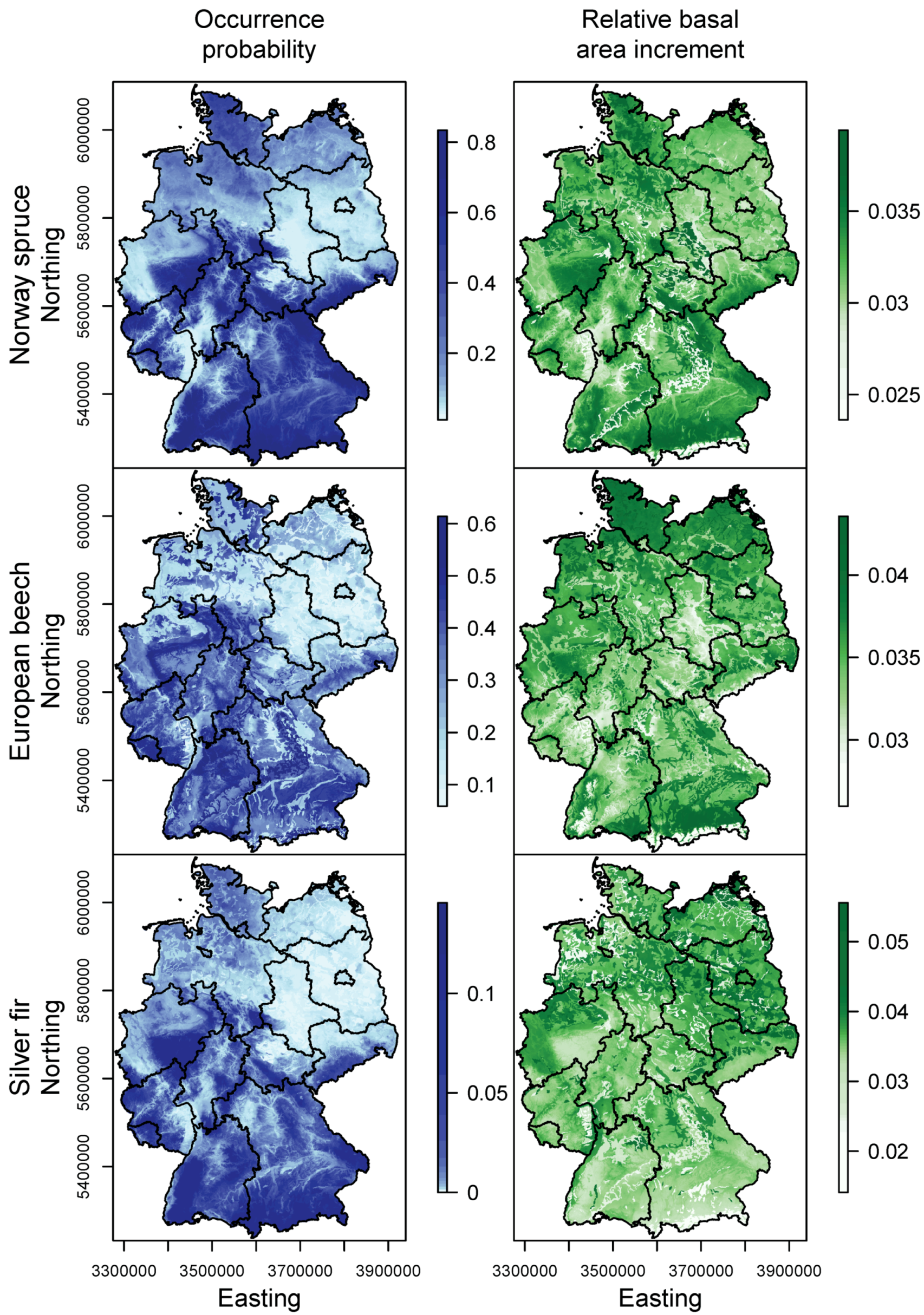
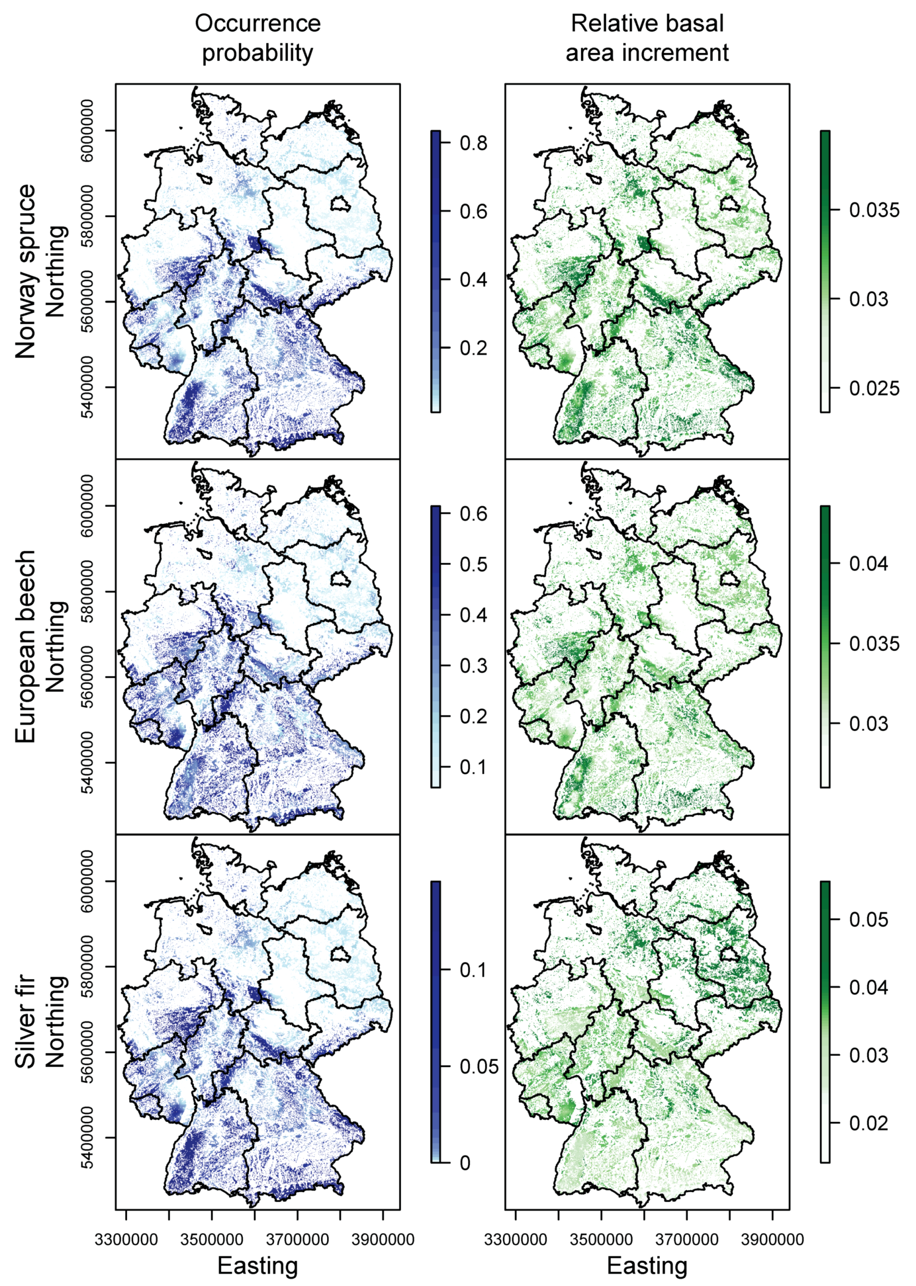
Growth and distribution were weakly correlated, indicating that they were proxies for different aspects of site suitability (Figure A2). For Norway spruce, an occurrence optimum was found in cool and humid conditions. Good growth conditions were modeled for an average precipitation sum of about 1300 mm and a temperature around 7 C. High occurrence probabilities were projected for low mountain ranges and high elevations (Figure 2 and Figure A4). In contrast to high occurrence probabilities at very high altitudes such as in the Alps, growth was very low due to the negative effect of low temperature. Apart from these regions, high occurrence probability was well-suited to good growing conditions.
Species distribution and growth were positively correlated for beech for parts of the climatic range (Figure A2). Low values were projected for low temperature and low precipitation relative to the species’ range, whereas high values were projected for high temperature and intermediate precipitation (up to 1400 mm). In more detail, occurrence probability was lower at the dry end of the observed precipitation gradient for the entire temperature range. Beech distribution resembled spruce distribution in wide parts, apart from high mountains (Figure 2 and Figure A4). In some areas with high occurrence probability due to a cool and moist climate, growth was low, but in most parts of Germany, its distribution and growth patterns were largely congruent.
For silver fir, high occurrence probability was modeled for high precipitation and warmer temperatures than spruce (Figure A2). In contrast to occurrence, good growth was predicted for decreasing precipitation. However, at the very dry end of the gradient, silver fir did not occur. The effect of temperature was rather weak but positive. The poor congruence of growth and occurrence also appeared in the spatial pattern: Silver fir distribution did not coincide well with optimal growth conditions (Figure 2 and Figure A4). Growth was low in higher elevations where strong occurrence was projected. A similar spatial distribution pattern was projected for spruce and beech, which was concentrated on mountain regions.
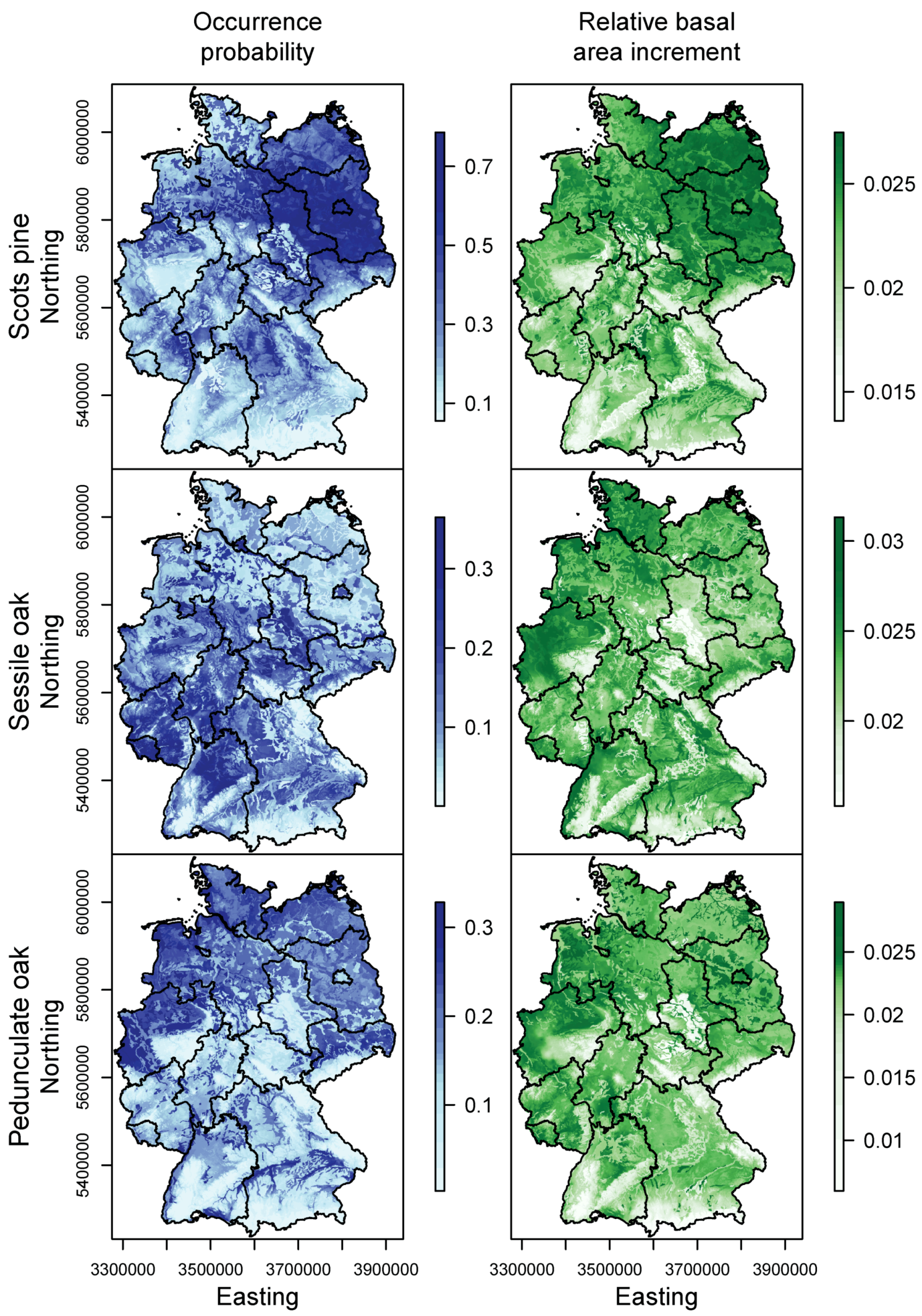
The other three species—Scots pine, sessile and pedunculate oak—were distributed in warmer areas. For Scots pine, stronger growth as well as a higher occurrence probability were modeled for warmer and drier conditions (Figure A2). Regions with higher occurrence probability also showed good growth (Figure 2 and Figure A4). Main occurrences were at low altitudes such as the North German Plain, the Upper Rhine Valley, or Central Franconia. Scots pine can be considered the most drought tolerant out of the six considered tree species.
For sessile oak, high occurrence probability was modeled for warm conditions and low to intermediate precipitation (Figure A2), not reaching the very dry end of Germany’s climatic gradient. The distribution ranged over the entire German mid-elevation area, the Southwest German Escarpments and the foothills of the Alps (Figure 2 and Figure A4). This pattern was similar to that of European beech, but sessile oak occurred less in the southern regions and with the higher low range mountains being spared. Under warm conditions, stronger growth for sessile oak was modeled. Growth was best at intermediate precipitation, but it did not show any clear optimum across the climatic gradient examined. Growth was particularly strong on the Lower Rhine, but was relatively high in the entire area.
Pedunculate oak distribution showed similarities to that of Scots pine. However, its occurrence optimum was shifted towards warmer temperatures (Figure A2). For the whole North German Plain and the river valleys of the alpine foothills and the Rhine-Main area, high occurrence probabilities were projected (Figure 2 and Figure A4). The distribution optimum of pedunculate oak was more congruent with good growth conditions than that of the sessile oak. Strong growth was largely in line with high occurrence probability, although relatively strong growth was also found in the Palatinate-Saarland Escarpment, the Main catchment area, and the state of Baden-Württemberg in the Neckarland. In spite of similar responses, there were great differences in the spatial pattern of the sessile oak and the pedunculate oak occurrence probabilities.
3.2. Happy Tree Index and Climate Change Projections
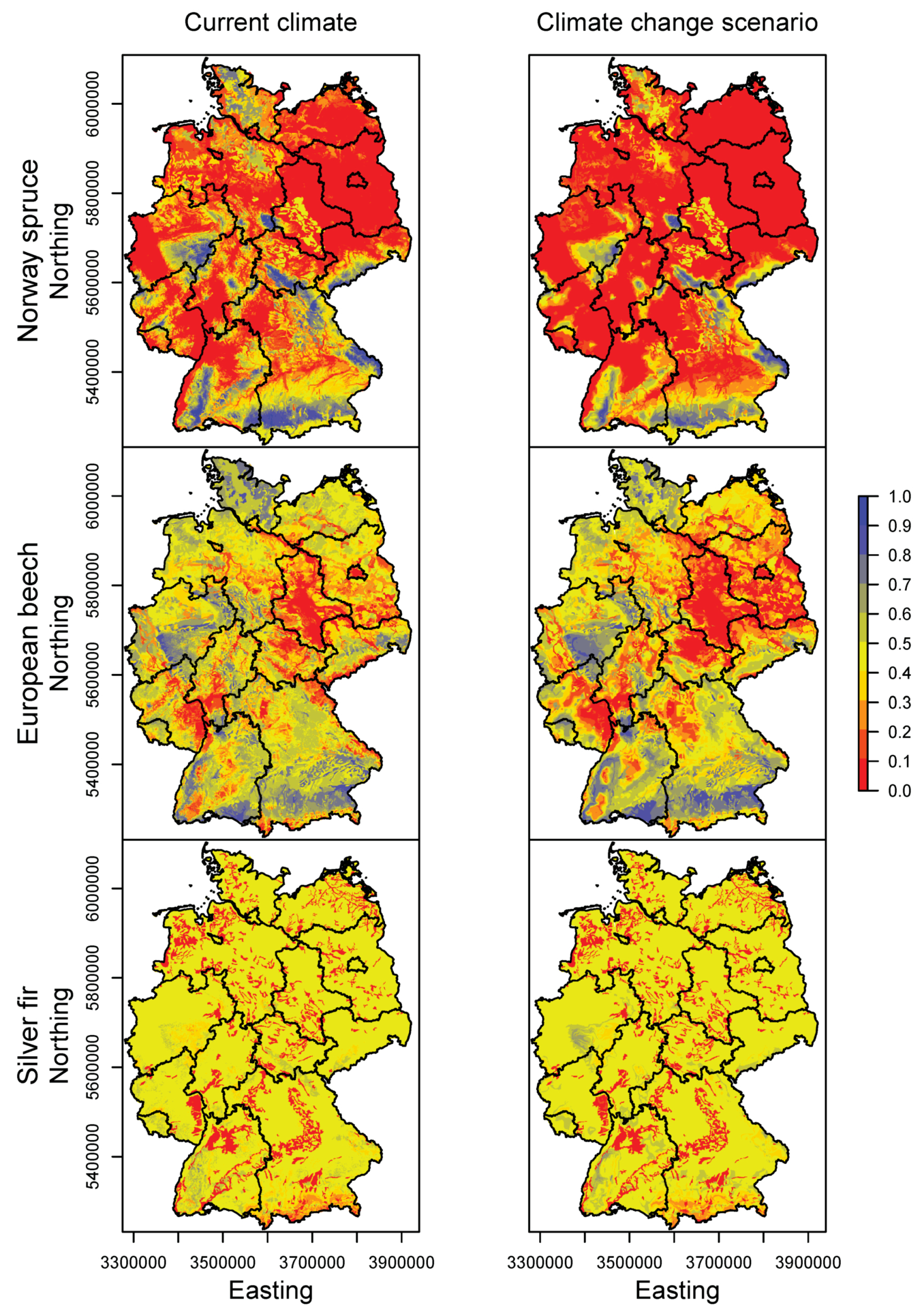
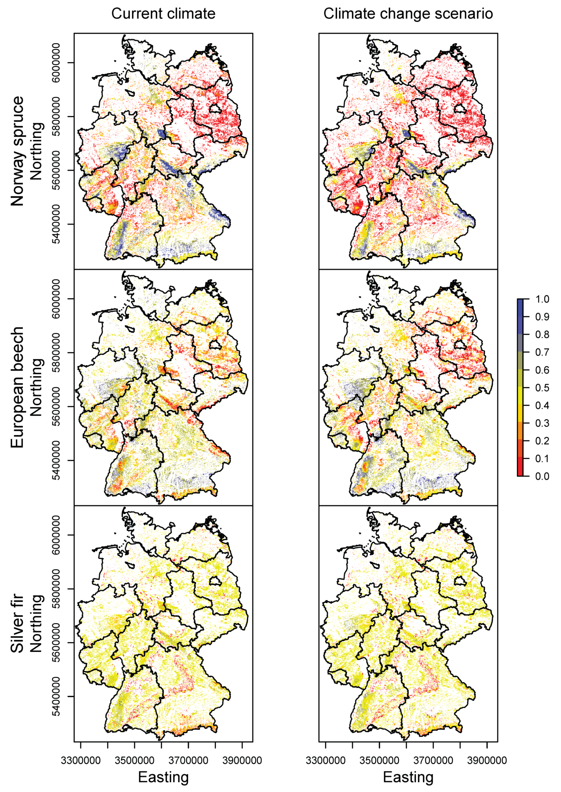
The HTI was used to combine occurrence probability and tree growth projections (Figure 2, Figure 3, Figure A3 and with forest mask Figure A4, Figure A5, Figure A6). According to the HTI, Norway spruce found the best conditions in the low range mountains and in northwestern Germany. The entire area of Germany, except very low areas, was marked as suitable. In the climate change scenario, only the low mountain ranges remained suitable. For most of Germany, conditions turned out to be unsuitable under climate change.
Suitable areas for European beech were found almost everywhere in Germany, except in northeastern Germany (Figure 3 and Figure A6). For the climate change scenario, we found lower suitability in northeastern Germany and generally at lower elevation. Contrary to spruce, for European beech, the German low mountain ranges and parts of northwest Germany remained favorable or improved sightly.
For silver fir, which co-occurs with spruce and European beech, intermediate conditions were identified all across Germany with the exception of some low mountain ranges. Under climate change, this pattern remained largely unchanged. This was caused by the contrary pattern and also the contrary development of the occurrence probability and growth (Figure 3). Occurrence probability increased for higher and decreased for lower elevations, whereas growth behaved contrarily.
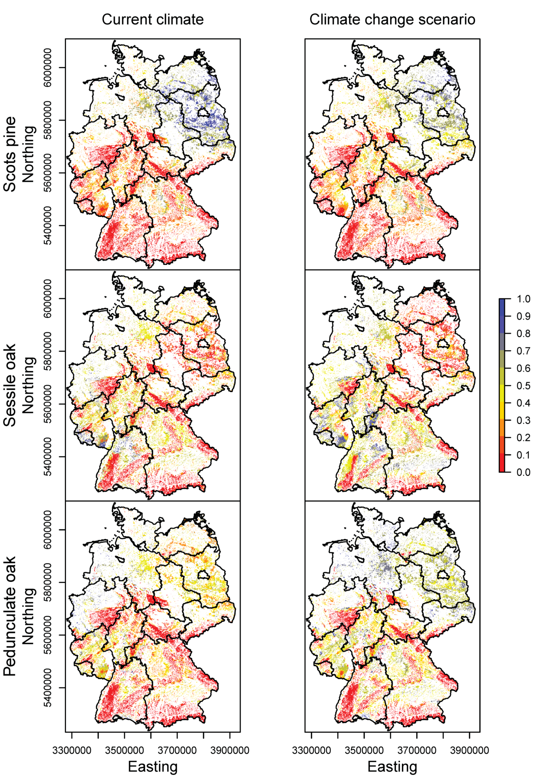
Scots pine showed the opposite pattern to spruce, European beech and silver fir (Figure 3 and Figure A6). Best conditions were projected for the northwestern lowlands whereas mountainous regions were unsuitable. Pedunculate oak, known to often accompany Scots pine, followed this pattern. Under climate change, Scots pine was not heavily affected, but HTI was decreasing in parts of the northwestern lowlands. Conditions for pedunculate oak, in contrast, improved for most areas classified as suitable today.
Regarding current conditions for sessile oak, low elevated areas were most suitable with a focus on central and western Germany, largely following the pattern of European beech. In the climate change scenario, we found a clear improvement of certain low elevated areas such as the Alpine foothills and some valleys. Some parts of the already unsuitable North German Plain became even worse.
3.3. Current Stands under Climate Change
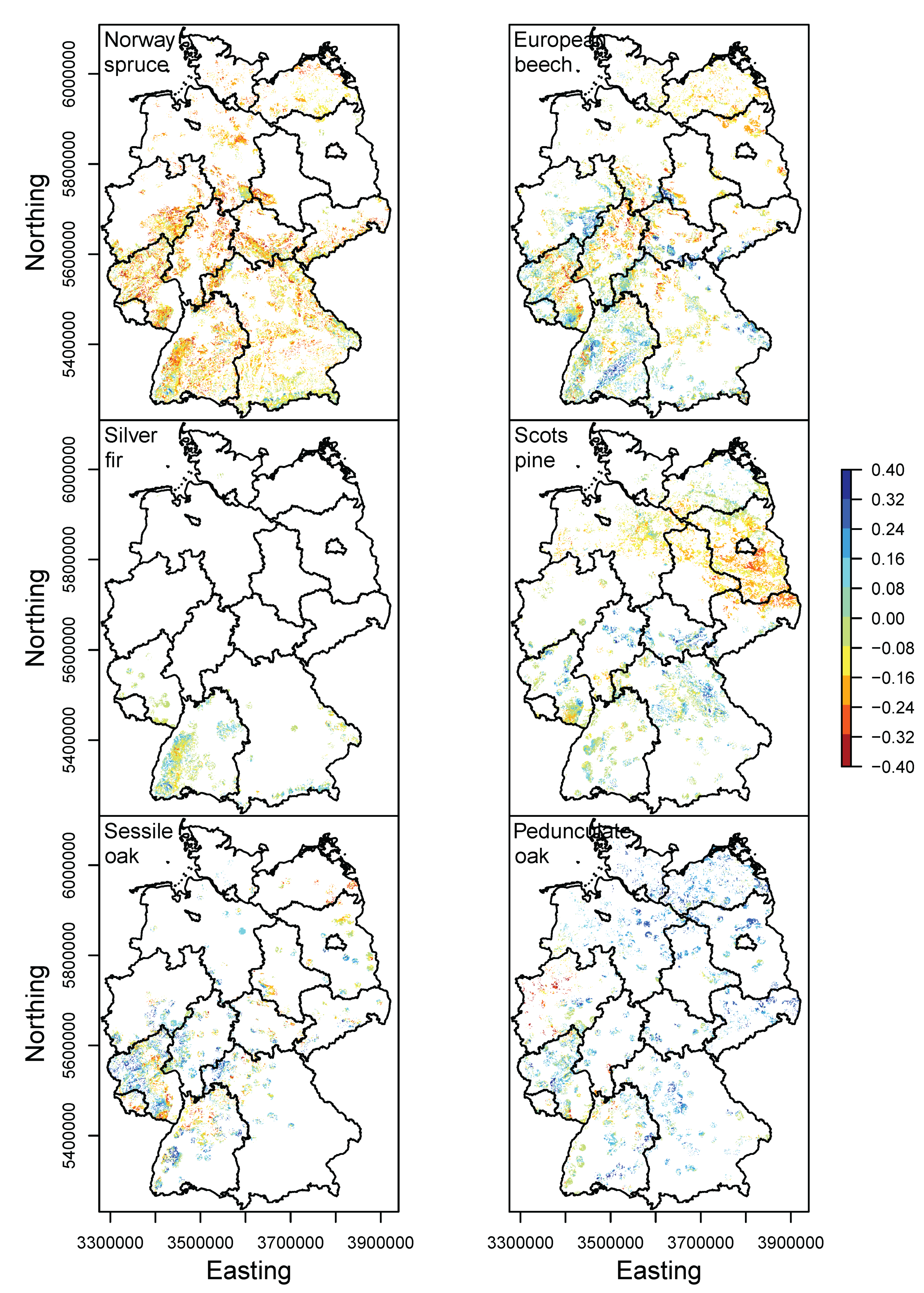
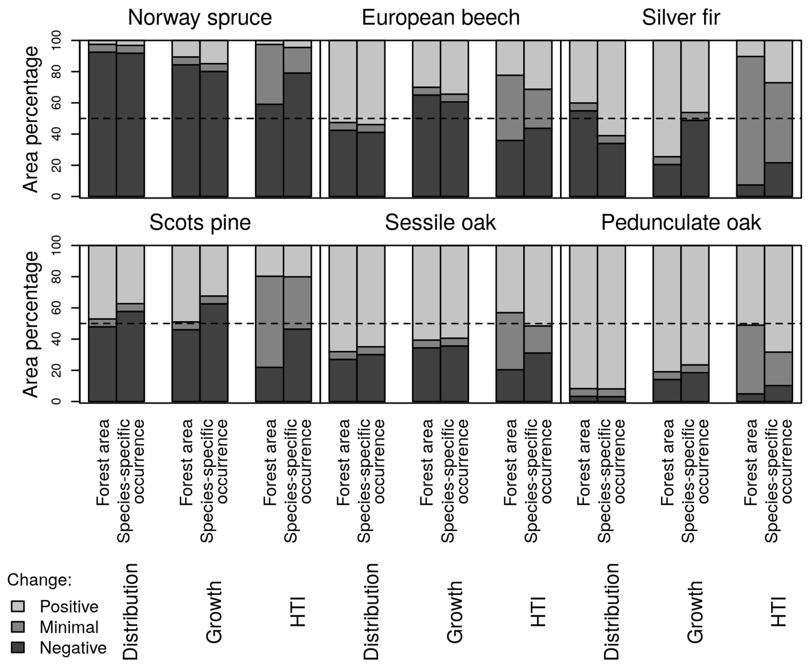
For Norway spruce, a large part of Germany showed negative changes of HTI (Figure 3). Isolating important stands showed indeed negative changes in site suitability, but not as dramatic as without the species mask, e.g., large parts of the very unsuitable North German Plain disappeared (Figure 4). At the highest elevations of mountain ranges and in the Alps, the modeled changes were close to zero. For species distribution, growth, and HTI, in about 90% of Germany’s forest area and current spruce stands, site suitability decreased under climate change (Figure 5). Remarkably, no clear positive changes were found. All federal states showed high negative changes in HTI (Table 3).
Just like Norway spruce, European beech showed the lowest HTI values in the climate change scenario where it was currently not important—particularly large parts of northeastern Germany (Figure 3). Most of the low mountain ranges remained unchanged and some even improved (Figure 4). Only European beech stands located at low elevation areas, especially in the northeast, showed strong negative changes. For beech, there was hardly any difference in considering forested area and species-specific area (Figure 5). Occurrence probability increased for half of the European beech stands. This differed from growth, for which negative changes predominated (60%). In terms of HTI, about 20% of the area improved and 40% declined, but absolute changes in HTI were rather small. Eight federal states showed more negatively and four showed more positively changing area, regardless of the intensity of the changes (Table 3).
Silver fir was the rarest species and had intermediate HTI values all over Germany (Figure 3). Therefore, stands in which it was considered to be an important species were also fewest. However, this species was modeled to experience mostly positive changes in site suitability under climate change (Figure 4). Its main occurrences were located in the Black Forest (Figure 4). For 30% to 55% of the area, occurrence probabilities decreased, depending on the considered subset (Figure 5). Negative changes were not very pronounced. For the species-specific area, negative changes were less than considering the whole forest area. In contrast, for growth, negative changes were larger for the species-specific area than considering the whole forest area (50% and 20%). Counter-intuitively, most of the area remained unchanged in terms of HTI. Considering the species-specific area, HTI increased in approx. 30% of the area, whereas for the forested area it increased only in 10% of the area. For Bavaria and Baden-Württemberg, 30–32% of the species-specific area improved in HTI (Table 3). Silver fir did not occur in the northern federal states.
For Scots pine, site suitability in terms of HTI in the North German Plain hardly changed in the northern half and changed negatively in the southern part (Figure 4). For the forested area, the share of improving versus decreasing conditions for occurrence and growth was balanced (Figure 5). The proportion of positively changing area declined by refining the considered area subset from the forested area to the species-specific area. Surprisingly, for more than half of the Scots pine stands, site suitability decreased. With 71%, Thuringia showed the largest positive HTI change for current Scots pine stands (Table 3). High positive changes were also found in Bavaria and Hesse with 42% and 45%. The largest negative change of 86% was found in Brandenburg. In Saarland, the negative change was 92%, but the species only had few important stands there and this federal state is quite small.
In southwestern and western Germany, where sessile oak was relatively frequent, there were areas with positive and areas with negative changes in HTI (Figure 4). Growth and occurrence conditions improved for around 60% of the forest as well as the species-specific area (Figure 5). More than 50% of the species-specific area increased in HTI. Approx. 20% remained unchanged. Eight federal states showed more positively than negatively changing area (Table 3). The largest negative changes were found in Saarland and Mecklenburg-West Pomerania with 49–91%, but in Mecklenburg-West Pomerania it was not very common. The largest positive changes were found in Bavaria, Hesse, North-Rhine Westphalia, Schleswig-Holstein, and Lower Saxony with up to 76%, but it was not very frequent in the latter two. In total, 52% of the forest area in Germany improved in site suitability (HTI).
The species-specific area of pedunculate oak was almost equally distributed across Germany (Figure 4). Most of these stands showed positive or no changes. About 75% of the area improved, whereas only about 10% declined in growth and occurrence conditions for both area subsets (Figure 5). Only 10% of the area changed negatively in HTI. In almost all federal states, the share of negative change in HTI was very low (Table 3). The highest positive changes were found in Brandenburg, Saxony, Mecklenburg-West Pomerania, and Schleswig-Holstein with up to 91%. The highest negative change with 38% was found in North-Rhine Westphalia as well as in Saarland, but it was not very important in the latter.
In summary, when only actual occurrences were considered, most of the species-specific relevant stands improved or remained unchanged for silver fir and both oak species and became worse for spruce. For European beech and Scots pine, there were positive as well as negative changes, thus, a spatially explicit assessment is mandatory.
3.4. Priority Regions
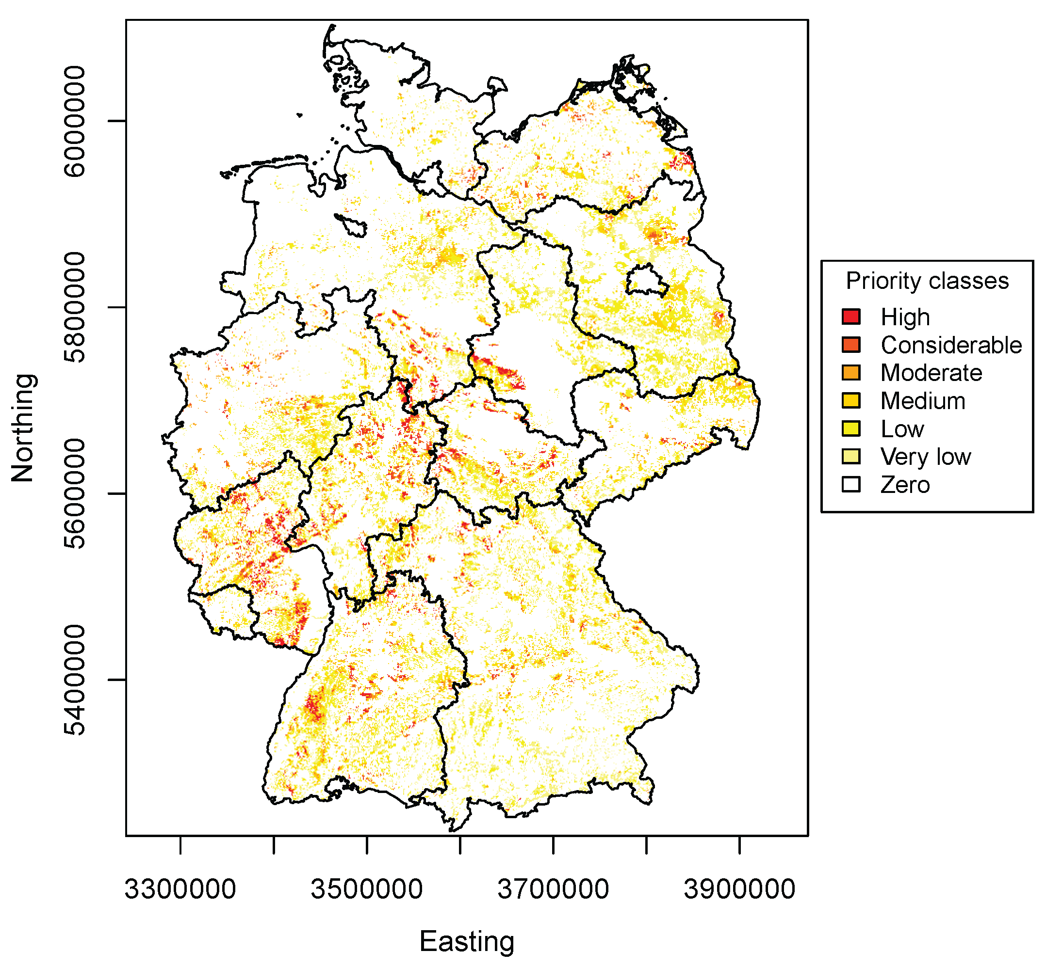
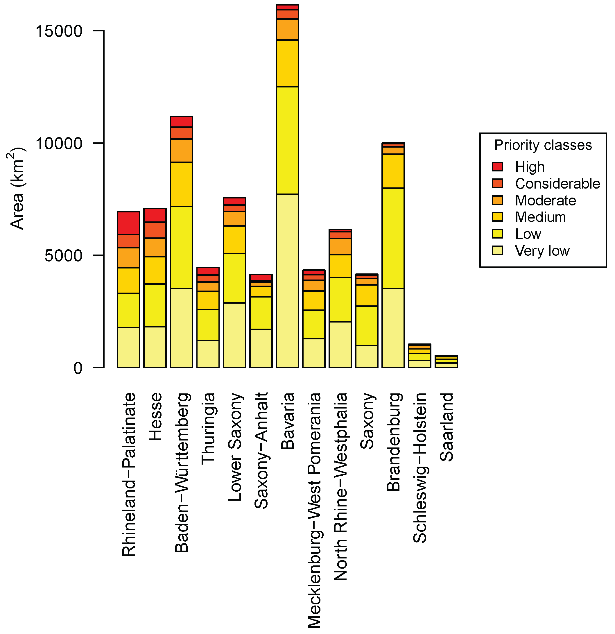
Priority regions were defined by expected strong negative change of site suitability (HTI) under climate change, summed up for all species and under consideration of current stands and forested area. Priority regions for climate change adaptation in Germany were mainly found in mid to low elevation regions, whereas higher areas such as the low mountain ranges showed less priority regions. Accordingly, central, western, and southwestern Germany were projected to experience stronger negative changes than the other regions (Figure 6). The largest absolute areas of priority regions were found in Rhineland-Palatinate, Hesse, Baden-Württemberg, Thuringia, Lower Saxony, and Saxony-Anhalt (Figure 7). By far the largest area with negative changes was found in Bavaria, however, with only a small share of priority regions. Most of the negatively changing area changed only weakly. Additionally, Bavaria is a large federal state with plenty of forest area. In contrast, Rhineland-Palatinate and Hesse do not belong to the largest federal states, but they had the largest absolute area of priority regions and the share of strong negative changes was greater.
Norway spruce strongly influenced the pattern of priority regions (Figure 4 and Figure 6). Additionally, low elevated European beech stands had a noticeable influence on the classification as priority regions. In the northern part of Baden-Württemberg, sessile oak contributed to priority regions to some extent. The other tree species contributed less to the priority regions since they were far less frequent and changes in site suitability were positive, neutral or only slightly negative.
4. Discussion
The aims of this study were to suggest a transparent and reproducible way to combine two aspects of site suitability, namely model projections for species distribution and tree growth, and to use this measure to identify priority regions for climate change adaptation under consideration of current stands. This was one of the first attempts to further develop the concept of site suitability in the field of climate impact modeling, and research should not be limited to these two proxies only [20]. Certainly, there were several steps in the workflow—starting at single species models and ending in a map of priority regions—at which we made decisions to be discussed. Nevertheless, we successfully calculated valid SDMs and growth models for the six main tree species of Germany and, thus, were able to provide spatial projections of changes in site suitability. Finally, we identified priority regions for climate change adaptation.
4.1. Current Site Suitability
The first step in providing an index for site suitability was the development of reliable models for its aspects; here, they were species occurrence probability as a proxy for risk, and species-specific tree growth as a proxy for productivity. Naturally, maps for the combined site suitability in terms of HTI differed from species distribution maps as well as from growth maps. Thus, a naïve interpretation of each type of map for species site suitability would differ, e.g., for spruce in the Alps, the influence of low growth was also visible in the HTI and resulted in a low or intermediate site suitability, whereas occurrence probability showed high values, which could be interpreted as good site suitability. Another example is the current site suitability of European beech in the Southern Alpine Foreland. Although beech was not broadly represented there and subsequently modeled occurrence probability was moderate, species growth was modeled to be strong. A rather positive evaluation of site suitability according to the HTI of that region was a result of strong growth combined with intermediate occurrence probability. Where only one of the two components was high, the resulting HTI was not exceeding intermediate values. Only for sites for which both the distribution and growth model gave high values did the HTI approach its maximum. Our results showed that depending on the aspects of site suitability considered, evaluations of species suitability under climate change and subsequently management recommendations differed.
The way in which `importance’ was defined here was very simple and certainly influenced results, but at least followed a reproducible and transparent definition. Importantly, this step in processing priority regions is open to adaptation, similarly to the weighting of risk and productivity. The two variables could also be combined differently, e.g., by a two-dimensional color scheme. Such alternative methods would conserve more information, but at the same time they were more complex to interpret.
Integrating even more aspects of site suitability into the calculation of the HTI in the future is feasible and easy to implement as additional summands or slightly more complex in terms of a Bayesian belief network. Such consideration of more aspects will enable informed decisions. Derivation of a summarizing measure such as the HTI reduced complexity and made weighting of aspects transparent and reproducible. With the produced maps for each aspect of site suitability, it is easy to customize the weighting of the aspects, which is important for practical use. In this way, an index for site suitability such as the HTI can be dynamically created according to management objectives—whether risk- or productivity-oriented.
4.2. Winners and Losers under Climate Change
Considering species-specific occurrences, the comparison between HTI projections for the current climate and the climate change scenario showed large areas of negative change, especially for Norway spruce and also for European beech and Scots pine. Silver fir did not show large changing areas. The largest positively changing areas were found for sessile oak and pedunculate oak. Regarding only currently occurring species resulted in less dramatic maps than when the entire forested area or even the non-forested area of Germany was considered, which demonstrated the importance of masking forested area as well as species-specific occurrences. The consideration of the total forest area is useful since this area is available for forestry as a potential planting area. For the assessment of management effort needed, actual species occurrences need to be considered.
Less dramatic maps as a result of using the forest or species mask is good news since this means that species selection by foresters was already reasonable in the past. However, many areas in which Norway spruce was important were deceasing in suitability in the climate change scenario. European beech also showed considerable decrease for current stands. Most experts agree with a diminishing suitability of spruce in Germany in the course of climate change (e.g., [41]). With its high competitiveness and tolerance to soils with low water storage capacity, European beech could still remain an important tree species in German forestry despite the expected negative development of site suitability under climate change [41,42]. The decline of areas in which spruce and beech currently occur poses a major challenge as large shares of the German timber production derive from these two species [43].
Also in earlier studies, a lower risk potential than for beech and spruce was found for silver fir [41]. This indicated that current stands with important shares of silver fir were thus well within its climatic range. Most of the area where silver fir was not identified to be important today showed low site suitability (HTI). However, the current distribution of this rare species showed a spatial pattern which was influenced by its postglacial migration [44], which is supported by paleontological findings [45], and by the silvicultural history in Germany. Hence, we assume that the current distribution of silver fir is not identical to its ecologically possible distribution. These facts make silver fir distribution and also growth difficult to model and, thus, the climatic niche was likely underestimated. Using other European NFIs could largely resolve this issue. Silver fir can be assumed to be a promising species also outside its current geographical range, because it is less susceptible to drought than spruce due to its deep root system and it is more resistant to storm damage [46]. Therefore, we conclude that silver fir has potential under climate change. However, other approaches such as long-term planting experiments need to be applied to provide final results. Most importantly, the influence of competitors, pathogens, or limitations in natural regeneration at sites where it grows well need to be considered.
For Scots pine, site suitability changed negatively in large areas. However, there were also areas with no or positive change. Negative changes of site suitability (HTI) were concentrated mainly in eastern Germany. Scots pine is an important species in German timber production, although this species does not grow as fast as spruce [40]. Its share of the German forest area has decreased slightly in recent years [40]. Furthermore, there are hints that Scots pine already experienced severe problems in dry areas [47], which was also found in our study. Some forest experts therefore re-evaluated the suitability of Scots pine in warm and dry areas [48,49]. However, the area that remained unchanged under climate change was larger for the whole forest area than for species-specific stands which means that the potential of Scots pine for climate change adaptation is not fully exploited yet.
Similar to Scots pine, the positive evaluation of both oak species in this study must be seen alongside their low yield which makes them unpopular for the German timber market. According to today’s opinion, oaks are well adapted to future conditions but are less competitive and do not show natural regeneration [49,50,51]. Additionally, pathogens for oaks could become more important in the face of climate change and, therefore, turn oaks into unfavorable species. A combination of different biotic and abiotic factors has already led to a decline in Central Europe during the last decades [52]. Nevertheless, we found a larger area with decreasing HTI for current stands than for the whole forest area for sessile oak. Hence, some more eligible sites might be found in the future for this species.
4.3. Priority Regions
Priority regions were mainly defined by decreasing site suitability of Norway spruce and European beech. The mid-range mountains were less affected than lower regions in general. Priority regions were not equally distributed across Germany, which was caused by different climatic conditions, but also determined by current stand forming species. Considering the absolute area classified as priority regions, the federal states Rhineland-Palatinate, Hesse, Baden-Württemberg, Thuringia, Lower Saxony, and Saxony-Anhalt were projected to be most affected. In Bavaria, Mecklenburg-West Pomerania, North-Rhine Westphalia, Saxony, Brandenburg, Schleswig-Holstein, and Saarland, less area was classified as priority regions compared to the other federal states. The total area with negative changes followed the order of total forest area to some extent, but with irregularities. This means that the share of negatively changing forest area of a federal state was not totally proportional to its forest area.
Comparing priority regions with results from other studies is challenging, because most studies on climate change projections of site suitability did not mask their maps—if any. Different methodologies in assessments of federal states render impossible a comparison of climate impact vulnerability over the whole area of Germany. Other studies, e.g., silvicultural risk maps [17], indeed focused on actually forested area but still did not consider species-specific occurrences. Some studies did not consider climate change scenarios but focused on currently already unsuitable sites which they expected to become worse earliest [53]. However, the relative area which was used to derive summaries on changes of species suitability under climate change differed depending on the area subset referred to. Projections for the entire area ignore the presence of other land cover types than forests. In contrast, projections masked by forested area provided information on actually available area for forestry under current constraints by other land cover types such as agronomy. Our approach to use a mask of species-specific important occurrences did not provide information on where to plant species today to adapt to future climatic conditions. Yet, it provided spatially explicit information on which regions in Germany need special attention due to strong negative projected changes for current stands.
Nevertheless, all federal states did regional assessments examining the vulnerability of their forests. Current forests of Baden-Württemberg were widely rated as vulnerable in a former study [54]. In this study, one of the largest area shares of priority regions was in fact found for Baden-Württemberg. However, not the whole forest area was affected equally. A large area with high priority was found in the Black Forest.
For Rhineland-Palatinate, contrary to us, a regional study evaluated the period until 2050 as not particularly severe [55]. Only a small area in the Rhine valley was considered as risky in this study, whereas we classified a larger area as priority regions concentrated in the central and southern parts of Rhineland-Palatinate. For a time period until 2070, the regional study found more risky areas in central and east parts of the federal state than for the time period until 2050.
For Bavaria, a regional study suggested focusing on warm and dry areas for forest conversion [56]. Priority regions followed this pattern, but were additionally identified in cold and humid areas.
For Hesse, low vulnerability of European beech, Scots pine and oaks, but great vulnerability for Norway spruce was projected [57], as also indicated by the priority regions in this study. However, we found a large share of priority regions in the northern part of Hesse which were characterized by European beech.
Due to an expected decline in water availability, high vulnerability was reported for northeastern Thuringia [58]. This area was also identified as a priority region by our analysis, and additionally, there were priority regions located in the east and in the west of Thuringia.
For Mecklenburg-West Pomerania, the lowest vulnerability was assessed for Scots pine, sessile oak and pedunculate oak; relatively low vulnerability was assumed for European beech; high vulnerability was assessed for Norway spruce [59]. However, priority regions for Mecklenburg-West Pomerania were characterized not only by the high vulnerability of spruce, but also by European beech. Furthermore, Scots pine contributed to priority regions in the south and sessile oak in the east.
Low vulnerability was assessed for the Scots pine- and pedunculate oak-dominated forests of Brandenburg [60]. In contrast, we found few priority regions in Brandenburg, which were mainly characterized by European beech and to a small extent by Scots pine.
A rather positive evaluation of North-Rhine Westphalia was concordant with regional studies, which predicted an improvement of beech in high elevation areas and a generally unproblematic trend for Scots pine and sessile oak [61]. The few priority regions were mainly characterized by pedunculate oak, which was considered a rather unproblematic species in the regional study. Norway spruce also contributed to the priority regions for North-Rhine Westphalia, which was in accordance with the regional study.
Both the location of our priority regions as well as, to a small extent, the causative species spruce and also beech agreed with a vulnerability assessment for Lower Saxony [62].
For Schleswig-Holstein, local studies declare spruce as the most vulnerable, beech as less vulnerable, and oaks and Scots pine as the least vulnerable [63], which was concordant with our findings.
It is highly appreciated that German federal states carry out studies to explore the vulnerability of their forests to climate change. The regional studies applied a variety of methods and approaches to estimate the vulnerability of forests to climate change. However, progress is slowed down by each state’s costly development of its own method. Despite the consistencies that occurred, the priority regions in this study did not always agree with the vulnerability analyses of the federal states and sometimes even contradicted them. This suggested that the selected method might have influenced the results. Some regional studies vaguely made general statements regarding certain species which may provide initial indications but they must be refined in order to effectively support management decisions. In our study, e.g., a single tree species could show quite a differentiated expected future suitability. A methodological standardization is desirable for better comparability among studies. Furthermore, a simple and reproducible method would be ideal.
4.4. Validity of HTI and Priority Regions
In this study, priority regions were defined on the basis of two models for proxies of site suitability (SDM and growth model), a concept for integration of their values (HTI), and a definition of `important species occurrences’ (Figure 1). At each of these steps in the workflow, decisions have been made and changes are possible.
At the first step, the decision to calculate SDMs and growth models instead of using tree abundance (number of stems, stem density), site index [14] or other variables which could be calculated based on NFI data, presumably influenced the results. Additionally, regardless of the response variables used, the definition of the model, i.e., how to consider repeated measurements and the nested sampling design of the German NFI, needed careful attention. Using weights and a marginal model is not the best way from the statistical point of view, but considering the size of the dataset and constraints in terms of the lack of an effective algorithm and computation resources, it was the best choice.
The second step was a reduction of the information to only one dimension. In doing so, implicit weighting was applied in the way that thresholds for classes were calculated. One could argue that this step was not necessary. However, before combining occurrence probabilities—depending on the prevalence of the species in the study region—and growth—which strongly differs among species—some kind of `standardization’ needs to be applied to avoid an uncontrolled different weighting depending on species-specific ranges of values. We decided to use a method based on thresholds which was previously used in tree species site suitability modeling [18] and applied an analogous approach for growth. Nevertheless, an ecologically meaningful standardization and remaining with a continuous variable would be preferable. Alternatively, one could stay with the two dimensions and deal with the complexity in interpretation.
Less complex is the implementation of a flexible weighting for each aspect of site suitability. For combination of SDM and growth model predictions, we used the mean of the two. However, a weighted mean could also be applied. Weights could be set individually and even be species-specific. This enables each user to decide individually. Additionally, the prediction uncertainty of each aspect could be included as up- or down-weighting according to the uncertainty of the information. Thereby, large differences in model reliability due to, e.g., data availability, could be accounted for.
Not of minor importance is the way in which important occurrences of species were defined. In this study, the 75% quantile of a species’ basal area share in the NFI data was used. Selecting another threshold, another dataset, or another concept will change the spatial pattern. The method of marking areas as important occurrences for one species with the help of species-specific basal area share up-weighted the influence of rare species compared to, e.g., using dominance.
Finally, priority regions depend on the selected climate change scenario and the methodology with which the data were produced. A more optimistic scenario or the usage of other algorithms might influence results.
However, we feel confident about the modeled tendencies and the usefulness of this approach. The idea to combine several sources of information and to mask change maps by important occurrences for each species in order to identify priority regions for climate change adaptation is a step forward in climate impact modeling as a management support.
5. Conclusions
Good estimates for climate-dependent site suitability are the basis for forest management under climate change. We suggested considering both species occurrence probabilities derived from its current distribution as a proxy for risk, and individual, species-specific tree growth as a proxy for productivity. Our results emphasized that the use of different proxies for site suitability changes management recommendations. A simple index such as the HTI can be easily extended with any number of other aspects of site suitability by adding more layers, e.g., disturbances such as wind throw or bark beetle risk. A consideration of more aspects will enable informed decisions. The derivation of a summarizing measure such as the HTI reduces complexity and makes weighting of aspects transparent and reproducible.
It is important to consider current stands to estimate the actual need for action. For Germany, our estimates of the exposure of actual stands to negative climate impacts were less dramatic than those suggested by studies on the potential changes in site suitability. Identifying priority regions under consideration of actual stands using a transparent index provides the opportunity for cost- and time-efficient adaptation of forest in the face of climate change. Its geographically broad application enables a comparison and prioritization of adaptation measures all over Germany, and among federal states.
Supplementary Materials
The following are available online at www.mdpi.com/1999-4907/8/6/181/s1, GeoTIFF files for maps: SDM (current climate), growth (current climate), HTI (current climate, climate change scenario; including species distribution and growth components separately), species-specific HTI change, and priority regions.
Acknowledgments
The study was funded by Landesanstalt für Umwelt, Messungen und Naturschutz Baden-Württemberg (LUBW). We thank Axel Albrecht and Dominik Cullmann from the Forstliche Versuchs- und Forschungsanstalt Baden-Württemberg (FVA BW) for fruitful discussions. We acknowledge support by Deutsche Forschungsgemeinschaft and Open Access Publishing Fund of Karlsruhe Institute of Technology. This work was in part performed on the computational resource bwUniCluster funded by the Ministry of Science, Research and Arts and the Universities of the State of Baden-Württemberg, Germany, within the framework program bwHPC.
Author Contributions
K.D. conceived the study; U.M. analyzed the data, developed and interpreted the models; U.M and K.D. wrote the paper.
Conflicts of Interest
The authors declare no conflict of interest.
Appendix A

Table A1.
Overview of the number of data points used, broken down by tree species and model.
| Species Distribution Model | |||||||
|---|---|---|---|---|---|---|---|
| Species | Data points Presence/Absence (Prevalence) | Temperature (C) Mean (min–max) | Precipitation (mm) Mean (min–max) | Soil Type (Most Frequent) | |||
| Norway spruce (Picea abies) | 19450/29327 (0.40) | 7.9 (2.6–10.8) | 1008 (499–2696) | Cambisol | |||
| European beech (Fagus sylvatica) | 16940/31837 (0.35) | 8.4 (2.6–11.0) | 908 (454–2503) | Cambisol | |||
| Scots pine (Pinus sylvestris) | 14220/34557 (0.29) | 8.8 (3.5–10.9) | 733 (471–2300) | Cambisol | |||
| Sessile oak (Quercus petraea) | 5716/43061 (0.12) | 8.8 (6.8–10.9) | 819 (458–1811) | Cambisol | |||
| Pedunculate oak (Quercus robur) | 5291/43486 (0.11) | 8.9 (6.1–11.0) | 755 (454–1902) | Cambisol | |||
| Silver fir (Abies alba) | 3161/45616 (0.06) | 7.8 (2.6–10.8) | 1285 (590–2575) | Cambisol | |||
| Growth model | |||||||
| Species | Data Points | Temperature (C) Mean (min–max) | Precipitation (mm) Mean (min–max) | Soil Type (Most Frequent) | Relative Basal Area Increment Mean (min–max) | Diameter at Breast Height (mm) Mean (min–max) | Stand Basal Area (m2/ha) Mean (min–max) |
| Norway spruce | 134151 | 8.2 (2.9–11.5) | 1106 (509–2745) | Cambisol | 0.037 (0–0.976) | 320 (70–1231) | 43.8 (4.0–125.0) |
| European beech | 70235 | 8.9 (2.9–11.5) | 955 (535–2590) | Cambisol | 0.03 (0–0.707) | 366 (70–1587) | 35.4 (4.0–122.8) |
| Scots pine | 55622 | 9.3 (3.1–11.7) | 767 (513–2391) | Cambisol | 0.027 (0–1.037) | 304 (76–899) | 37 (4.0–108.3) |
| Sessile oak | 13947 | 9.5 (7.3–11.5) | 823 (456–1905) | Cambisol | 0.023 (0–0.483) | 362 (70–1100) | 34.4 (4.0–97.3) |
| Pedunculate oak | 10532 | 9.5 (7.1–11.6) | 777 (509–1890) | Cambisol | 0.026 (0–0.828) | 439 (70–1432) | 32.9 (4.0–110) |
| Silver fir | 14719 | 8.3 (2.9–11.3) | 1319 (618–2635) | Cambisol | 0.033 (0–0.665) | 420 (70–1277) | 43.9 (4.0–107.3) |
Table A2.
Thresholds for the formation of ecologically meaningful classes for the modeled occurrence probability and growth (annual relative basal area increment). We used the method of Hanewinkel et al. (2014) [18] for occurrence probability. The three thresholds TV1, TV2 and TV3 were supplemented by two more to allow a more differentiated representation. This proved particularly useful in the calculation of the combined site suitability. According to the number of thresholds for occurrence probability, the thresholds for growth were determined using 1/6 quantiles.
| Threshold | Description | Norway Spruce | European Beech | Silver Fir | Scots Pine | Sessile Oak | Pedunculate Oak |
|---|---|---|---|---|---|---|---|
| Species distribution model | |||||||
| tv1 | Value for which false positive rate <1% | 0.80 | 0.58 | 0.43 | 0.70 | 0.37 | 0.30 |
| tv11 | Value for which false positive rate <10% | 0.64 | 0.48 | 0.23 | 0.48 | 0.29 | 0.26 |
| tv2 | Value for which Kappa is maximum | 0.42 | 0.35 | 0.19 | 0.37 | 0.21 | 0.22 |
| tv31 | Value for which false negative rate <10% | 0.24 | 0.25 | 0.36 | 0.17 | 0.17 | 0.17 |
| tv3 | Value for which false negative rate <1% | 0.10 | 0.12 | 0.05 | 0.09 | 0.05 | 0.08 |
| Growth model | |||||||
| q1 | 1/6 quantile | 0.0319 | 0.0316 | 0.0298 | 0.0211 | 0.0210 | 0.0213 |
| q2 | 2/6 quantile | 0.0332 | 0.0328 | 0.0310 | 0.0230 | 0.0224 | 0.0222 |
| q3 | 3/6 quantile | 0.0342 | 0.0340 | 0.0323 | 0.0241 | 0.0233 | 0.0226 |
| q4 | 4/6 quantile | 0.0350 | 0.0354 | 0.0332 | 0.0253 | 0.0238 | 0.0231 |
| q5 | 5/6 quantile | 0.0360 | 0.0376 | 0.0341 | 0.0260 | 0.0245 | 0.0239 |
Figure A1.
Illustration of how to derive the happy tree index (HTI) from distribution and growth with equal weights of the two variables.
Figure A1.
Illustration of how to derive the happy tree index (HTI) from distribution and growth with equal weights of the two variables.

Figure A2.
Species responses for species distribution and growth for Cambisol (brown earth) and the species-specific median of stand basal area. Species responses for other soil types or stand basal areas show the same pattern, but show higher or lower values.
Figure A2.
Species responses for species distribution and growth for Cambisol (brown earth) and the species-specific median of stand basal area. Species responses for other soil types or stand basal areas show the same pattern, but show higher or lower values.
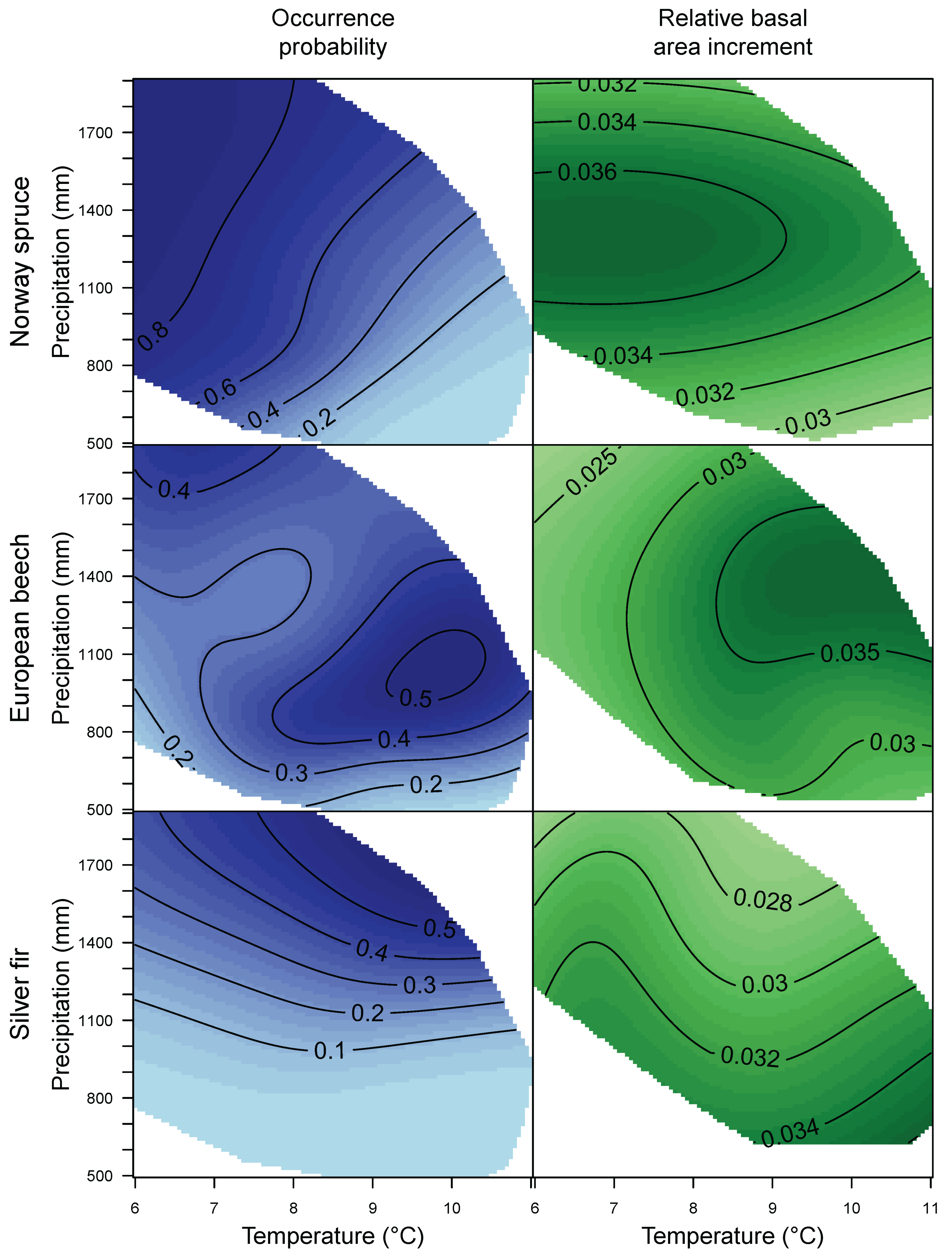
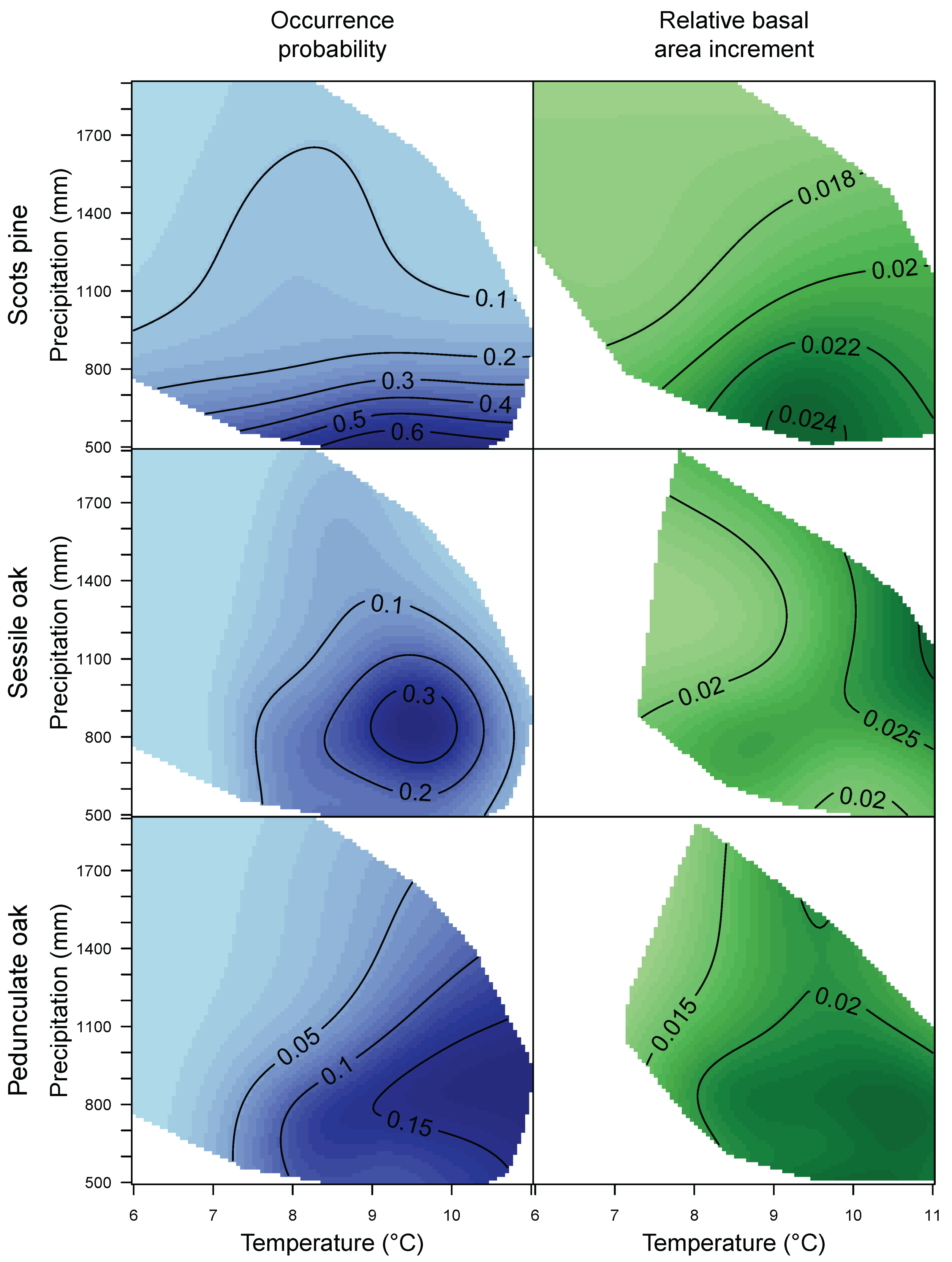
Figure A3.
Maps of Germany for the distribution and growth of six main tree species for the climate change scenario RCP 8.5 [29] until 2050. (Gauss Krueger coordinates, Zone 3; EPSG code: 31467).
Figure A3.
Maps of Germany for the distribution and growth of six main tree species for the climate change scenario RCP 8.5 [29] until 2050. (Gauss Krueger coordinates, Zone 3; EPSG code: 31467).
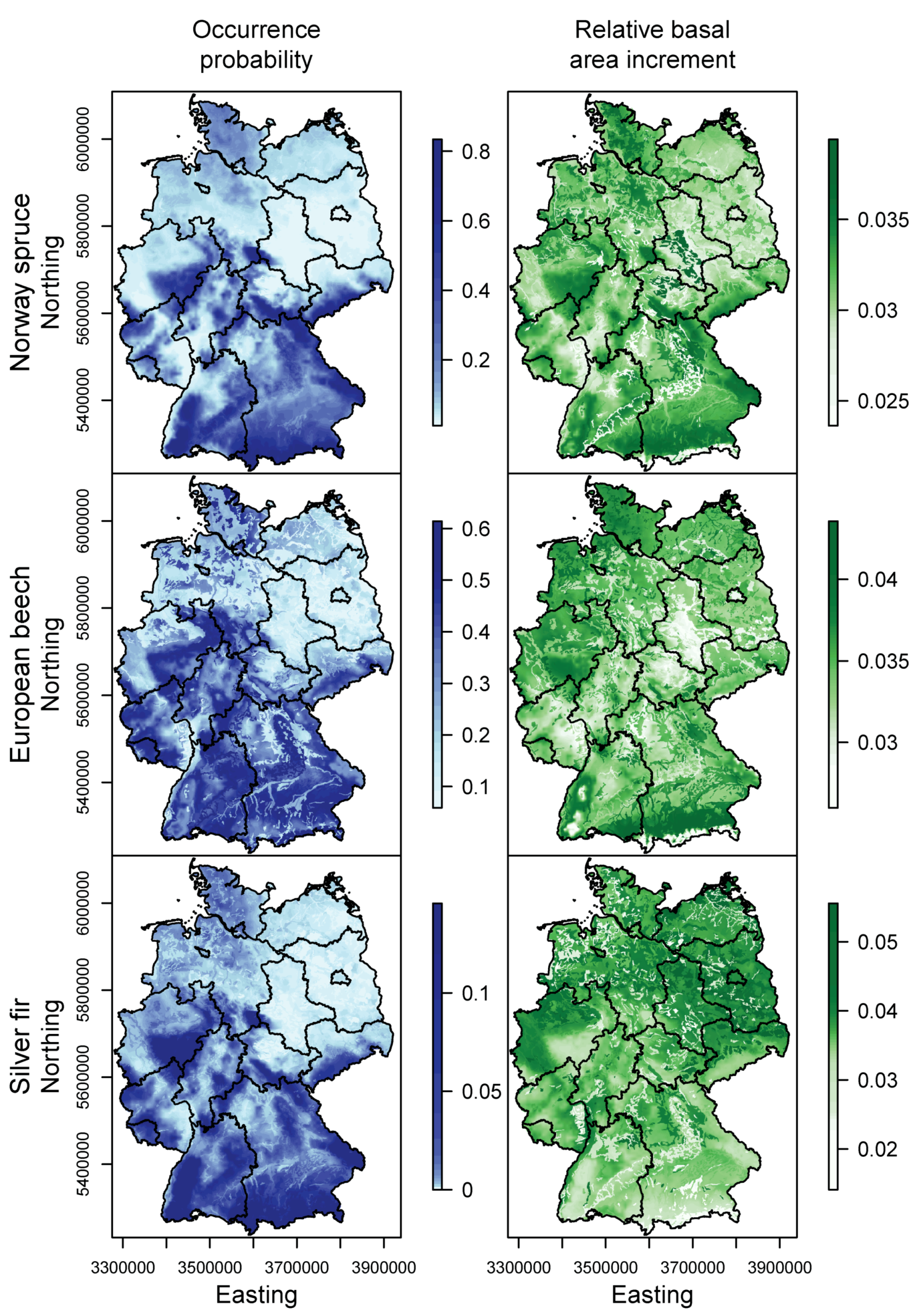
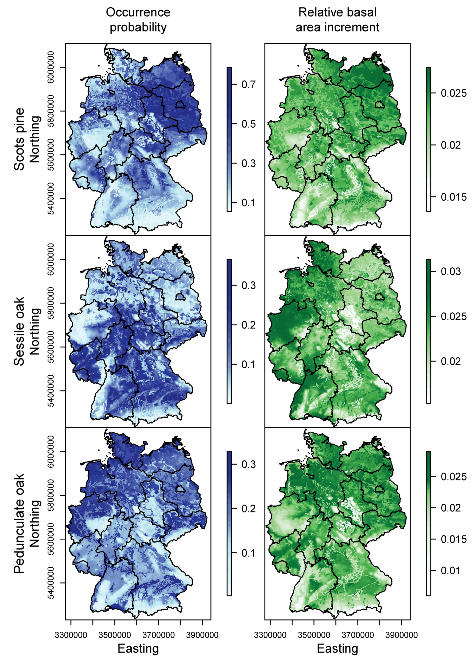
Figure A4.
Maps of Germany for the distribution and growth of six main tree species for the current climate. Only forested areas according to Coordinated Information on the European Environment (CORINE) land cover data [39] are shown. (Gauss Krueger coordinates, Zone 3; EPSG code: 31467).
Figure A4.
Maps of Germany for the distribution and growth of six main tree species for the current climate. Only forested areas according to Coordinated Information on the European Environment (CORINE) land cover data [39] are shown. (Gauss Krueger coordinates, Zone 3; EPSG code: 31467).
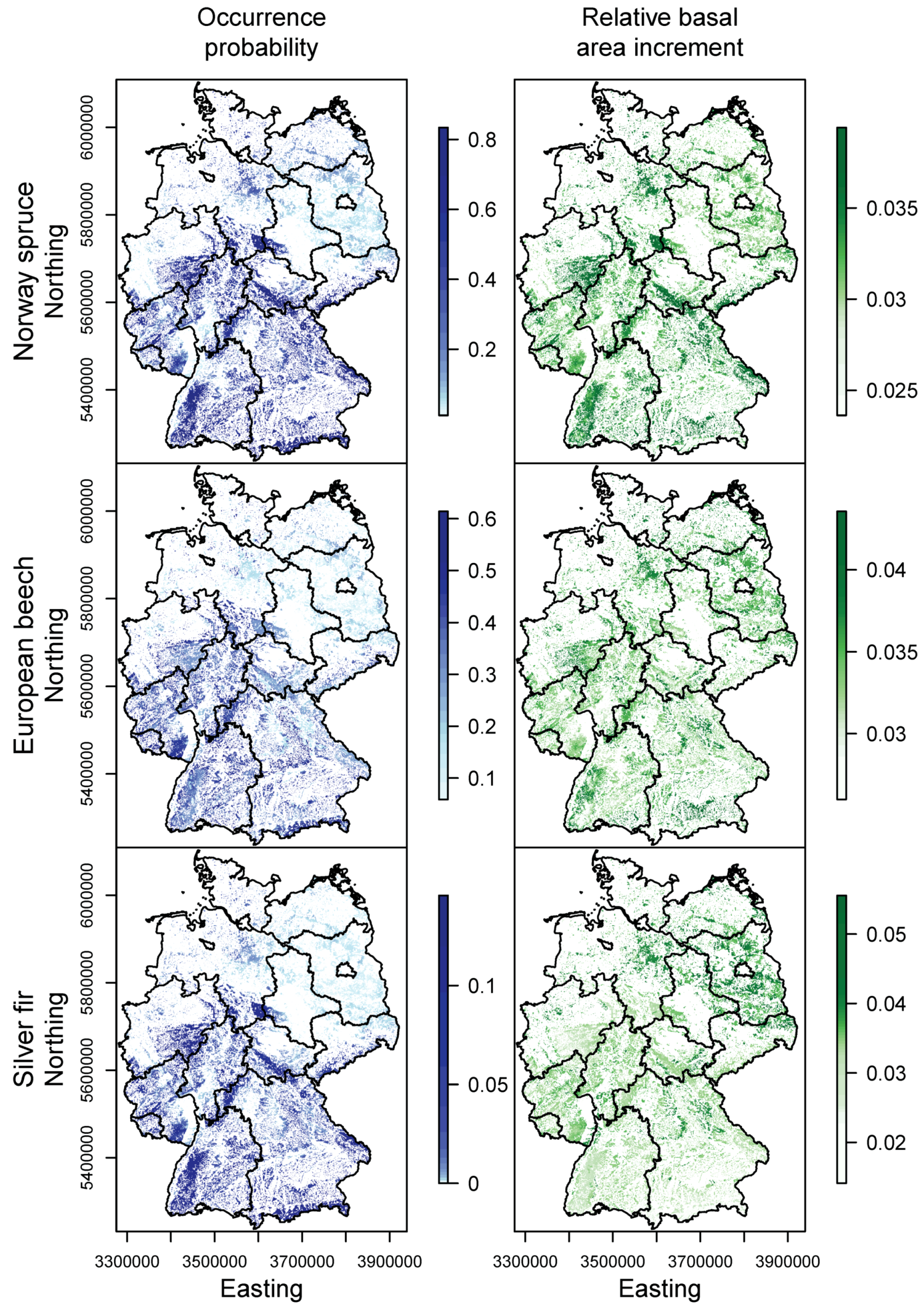
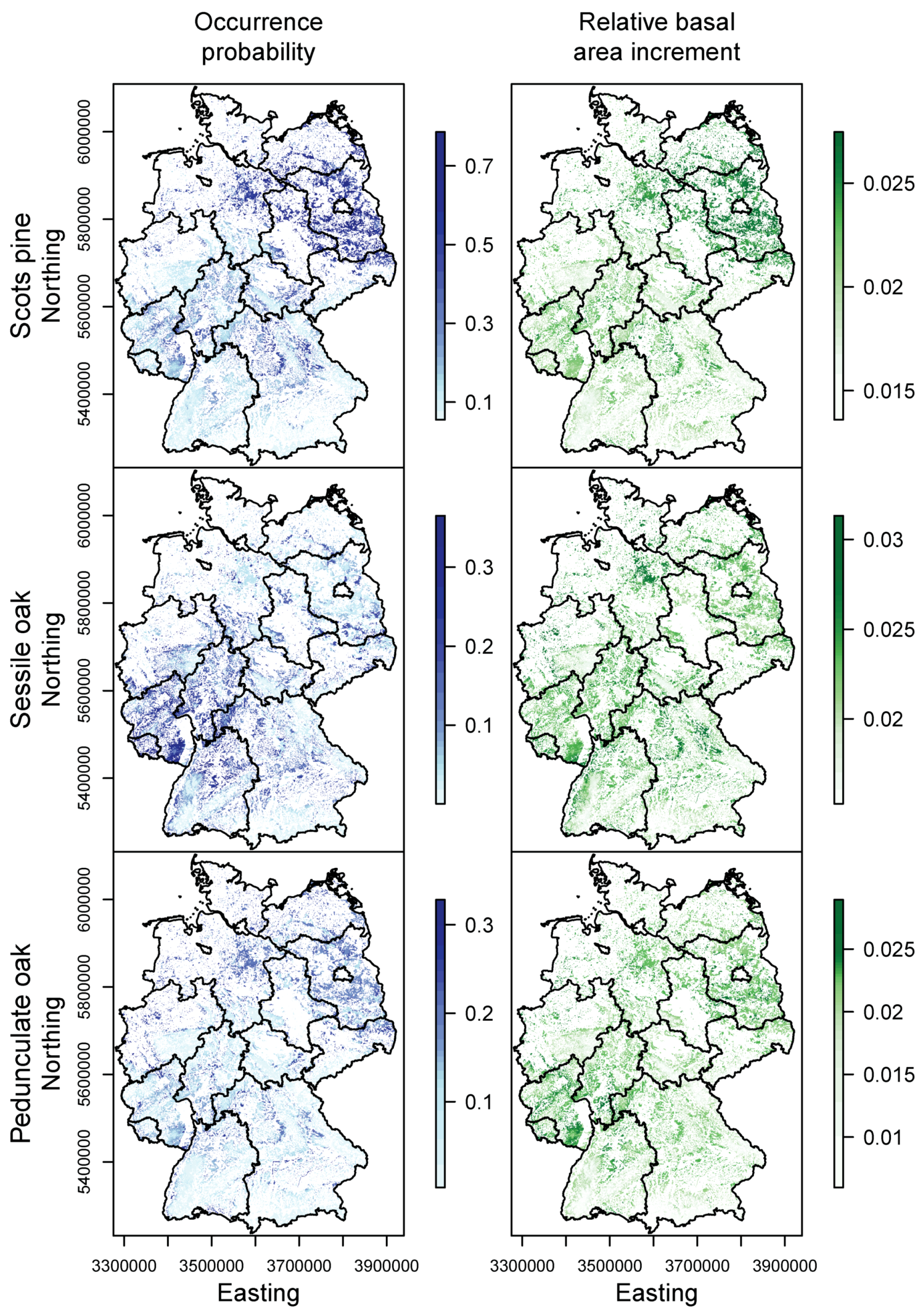
Figure A5.
Maps of Germany for the distribution and growth of six main tree species for the climate change scenario RCP 8.5 [29] until 2050. Only forested areas according to Coordinated Information on the European Environment (CORINE) land cover data [39] are shown. (Gauss Krueger coordinates, Zone 3; EPSG code: 31467).

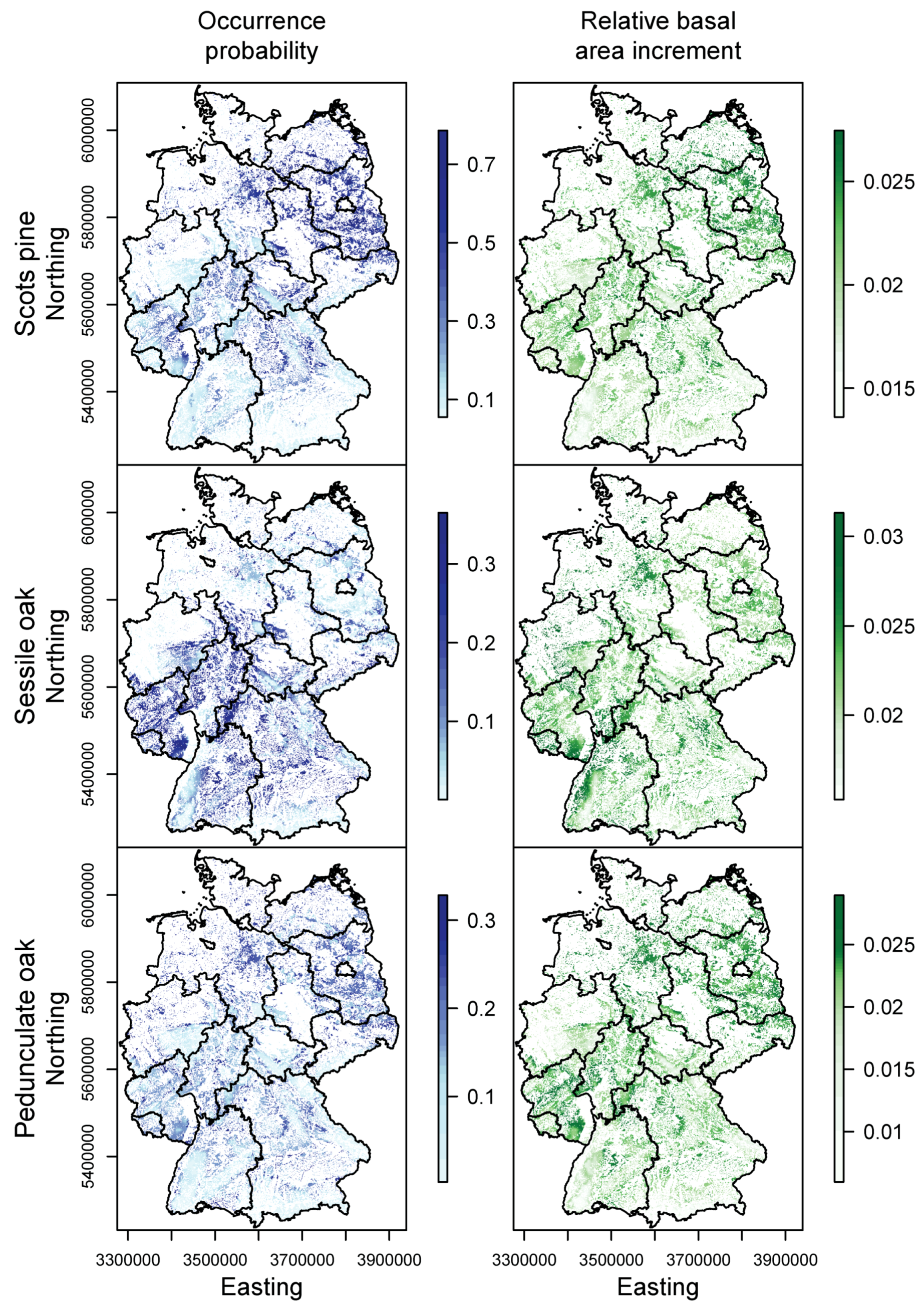
Figure A6.
Projections of the happy tree index (HTI) which combined species distribution and growth model projections. Regions in Germany can be identified, which are suitable or unsuitable under current and climate change scenario conditions. Only forested areas according to Coordinated Information on the European Environment (CORINE) land cover data [39] are shown. (EPSG code: 31467).
References
- Lindner, M.; Maroschek, M.; Netherer, S.; Kremer, A.; Barbati, A.; Garcia-Gonzalo, J.; Seidl, R.; Delzon, S.; Corona, P.; Kolström, M.; et al. Climate change impacts, adaptive capacity, and vulnerability of European forest ecosystems. For. Ecol. Manag. 2010, 259, 698–709. [Google Scholar] [CrossRef]
- Iverson, L.R.; Prasad, A.M. Predicting Abundance of 80 Tree Species Following Climate Change in the Eastern United States. Ecol. Monogr. 1998, 68, 465–485. [Google Scholar] [CrossRef]
- Thomas, C.D.; Cameron, A.; Green, R.E.; Bakkenes, M.; Beaumont, L.J.; Collingham, Y.C.; Erasmus, B.F.N.; de Siqueira, M.F.; Grainger, A.; Hannah, L.; et al. Extinction risk from climate change. Nature 2004, 427, 145–148. [Google Scholar] [CrossRef] [PubMed]
- Svenning, J.C.; Skov, F. Limited filling of the potential range in European tree species. Ecol. Lett. 2004, 7, 565–573. [Google Scholar] [CrossRef]
- Guisan, A.; Thuiller, W. Predicting species distribution: Offering more than simple habitat models. Ecol. Lett. 2005, 8, 993–1009. [Google Scholar] [CrossRef]
- Morin, X.; Thuiller, W. Comparing niche- and process-based models to reduce prediction uncertainty in species range shifts under climate change. Ecology 2009, 90, 1301–1313. [Google Scholar] [CrossRef] [PubMed]
- Purves, D.W. The demography of range boundaries versus range cores in eastern US tree species. Proc. R. Soc. B Biol. Sci. 2009, 276, 1477–1484. [Google Scholar] [CrossRef] [PubMed]
- Benito-Garzon, M.; Ruiz-Benito, P.; Zavala, M.A. Interspecific differences in tree growth and mortality responses to environmental drivers determine potential species distributional limits in Iberian forests. Glob. Ecol. Biogeogr. 2013, 22, 1141–1151. [Google Scholar] [CrossRef]
- Peng, C. From static biogeographical model to dynamic global vegetation model: A global perspective on modelling vegetation dynamics. Ecol. Model. 2000, 135, 33–54. [Google Scholar] [CrossRef]
- Albert, M.; Schmidt, M. Climate-sensitive modelling of site-productivity relationships for Norway spruce (Picea abies (L.) Karst.) and common beech (Fagus sylvatica L.). For. Ecol. Manag. 2010, 259, 739–749. [Google Scholar] [CrossRef]
- Charru, M.; Seynave, I.; Morneau, F.; Bontemps, J.D. Recent changes in forest productivity: An analysis of national forest inventory data for common beech (Fagus sylvatica L.) in north-eastern France. For. Ecol. Manag. 2010, 260, 864–874. [Google Scholar] [CrossRef]
- Gómez-Aparicio, L.; García-Valdés, R.; Ruíz-Benito, P.; Zavala, M.A. Disentangling the relative importance of climate, size and competition on tree growth in Iberian forests: Implications for forest management under global change. Glob. Chang. Biol. 2011, 17, 2400–2414. [Google Scholar] [CrossRef]
- Nothdurft, A.; Wolf, T.; Ringeler, A.; Böhner, J.; Saborowski, J. Spatio-temporal prediction of site index based on forest inventories and climate change scenarios. For. Ecol. Manag. 2012, 279, 97–111. [Google Scholar] [CrossRef]
- Brandl, S.; Falk, W.; Klemmt, H.J.; Stricker, G.; Bender, A.; Rötzer, T.; Pretzsch, H. Possibilities and Limitations of Spatially Explicit Site Index Modelling for Spruce Based on National Forest Inventory Data and Digital Maps of Soil and Climate in Bavaria (SE Germany). Forests 2014, 5, 2626–2646. [Google Scholar] [CrossRef]
- Kölling, C. Was wächst künftig wo? Klima-Risikokarten als Planungsunterlagen für den Waldumbau. Bayer. Landwirtsch. Wochenbl. 2009, 48, 58–60. [Google Scholar]
- Falk, W.; Mellert, K.H. Species distribution models as a tool for forest management planning under climate change: risk evaluation of Abies alba in Bavaria. J. Veg. Sci. 2011, 22, 621–634. [Google Scholar] [CrossRef]
- Falk, W.; Mellert, K.H.; Bachmann-Gigl, U.; Kölling, C. Bäume für die Zukunft: Baumartenwahl auf wissenschaftlicher Grundlage. Anbaurisikokarten jetzt um Boden- und Reliefparameter ergänzt. LWF Aktuell 2013, 94, 8–11. [Google Scholar]
- Hanewinkel, M.; Cullmann, D.A.; Michiels, H.G.; Kändler, G. Converting probabilistic tree species range shift projections into meaningful classes for management. J. Environ. Manag. 2014, 134, 153–165. [Google Scholar] [CrossRef] [PubMed]
- Polley, H.; Schmitz, F.; Hennig, P.; Kroiher, F. Germany. In National Forest Inventories—Pathways for Common Reporting; Tomppo, E., Gschwantner, T., Lawrence, M., McRoberts, R.E., Eds.; Springer: New York, NY, USA, 2010. [Google Scholar]
- Albrecht, A.T.; Fortin, M.; Kohnle, U.; Ningre, F. Coupling a tree growth model with storm damage modeling—Conceptual approach and results of scenario simulations. Environ. Model. Softw. 2015, 69, 63–76. [Google Scholar] [CrossRef]
- Thuiller, W.; Münkemüller, T.; Schiffers, K.H.; Georges, D.; Dullinger, S.; Eckhart, V.M.; Edwards, T.C.; Gravel, D.; Kunstler, G.; Merow, C.; et al. Does probability of occurrence relate to population dynamics? Ecography 2014, 37, 1155–1166. [Google Scholar] [CrossRef] [PubMed]
- Dolos, K.; Bauer, A.; Albrecht, S. Site suitability for tree species: Is there a positive relation between a tree species’ occurrence and its growth? Eur. J. For. Res. 2015, 134, 609–621. [Google Scholar] [CrossRef]
- Tinner, W.; Lotter, A.F. Holocene expansions of Fagus silvatica and Abies alba in Central Europe: Where are we after eight decades of debate? Quat. Sci. Rev. 2006, 25, 526–549. [Google Scholar] [CrossRef]
- Mauri, A.; de Rigo, D.; Caudullo, G. Abies alba in Europe: Distribution, habitat, usage and threats. In European Atlas of Forest Tree Species; Publication Office of the European Union: Luxembourg, 2016. [Google Scholar]
- Hansen, J.K.; Larsen, J.B. European silver fir (Abies alba Mill.) provenances from Calabria, southern Italy: 15-year results from Danish provenance field trials. Eur. J. For. Res. 2004, 123, 127–138. [Google Scholar] [CrossRef]
- Wykoff, W. A Basal Area Increment Model for Individual Conifers in the Northern Rocky-Mountains. For. Sci. 1990, 36, 1077–1104. [Google Scholar]
- Hijmans, R.; Phillips, S.; Leathwick, J.; Elith, J. Dismo: Species Distribution Modeling; R Package; 2016. [Google Scholar]
- Babst, F.; Carrer, M.; Poulter, B.; Urbinati, C.; Neuwirth, B.; Frank, D. 500 years of regional forest growth variability and links to climatic extreme events in Europe. Environ. Res. Lett. 2012, 7, 045705. [Google Scholar] [CrossRef]
- Moss, R.; Babiker, W.; Brinkman, S.; Calvo, E.; Carter, T.; Edmonds, J.; Elgizouli, I.; Emori, S.; Erda, L.; Hibbard, K.; et al. Towards New Scenarios for the Analysis of Emissions: Climate Change, Impacts and Response Strategies; Intergovernmental Panel on Climate Change Secretariat (IPCC): Geneva, Switzerland, 2008. [Google Scholar]
- Sedlmeier, K.; Schädler, G. Ensembles Hoch Aufgelöster Regionaler Klimasimulationen zur Analyse Regionaler Klimaänderungen in Baden-Württemberg und Ihre Auswirkungen; LUBW Landesanstalt für Umwelt, Messungen und Naturschutz Baden-Württemberg: Karlsruhe, Germany, 2015. [Google Scholar]
- Sedlmeier, K.; Mieruch, S.; Schädler, G.; Kottmeier, C. Compound extremes in a changing climate—A Markov Chain approach. Nonlin. Processes Geophys. 2016, 23, 375–390. [Google Scholar] [CrossRef]
- Panagos, P.; Van Liedekerke, M.; Jones, A.; Montanarella, L. European Soil Data Centre: Response to European policy support and public data requirements. Land Use Policy 2012, 29, 329–338. [Google Scholar] [CrossRef]
- Wood, S.N. Thin plate regression splines. J. R. Stat. Soc. Ser. B (Stat. Methodol.) 2003, 65, 95–114. [Google Scholar] [CrossRef]
- Akaike, H. A new look at the statistical model identification. IEEE Trans. Autom. Control 1974, 6, 716–723. [Google Scholar] [CrossRef]
- R Core Team. R: A Language and Environment for Statistical Computing. R Foundation for Statistical Computing; R Core Team: Vienna, Austria, 2016. [Google Scholar]
- Wood, S.N. Stable and efficient multiple smoothing parameter estimation for generalized additive models. J. Am. Stat. Assoc. 2004, 99, 673–686. [Google Scholar] [CrossRef]
- Hijmans, R.J.; van Etten, J. Raster: Geographic Analysis and Modeling With Raster Data; R Package Version 2.0-12; 2012. [Google Scholar]
- Heagerty, P.J.; Zeger, S.L. Marginalized multilevel models and likelihood inference. Stat. Sci. 2000, 15, 1–19. [Google Scholar]
- European Environment Agency. Corine Land Cover 2012; European Environment Agency: Copenhagen, Denmark, 2012. [Google Scholar]
- Polley, H.; Hennig, P.; Kroiher, F.; Marks, A.; Riedel, T.; Schmidt, U.; Schwitzgebel, F.; Stauber, T. Der Wald in Deutschland - Ausgewählte Ergebnisse der Dritten Bundeswaldinventur; Bundesministerium für Ernährung und Landwirtschaft (BMEL): Berlin, Germany, 2016. [Google Scholar]
- Kohnle, U.; Hein, S.; Michiels, H.G. Waldbauliche Handlungsmöglichkeiten angesichts des Klimawandels. FVA-Einblick+ 2008, 1, 53–55. [Google Scholar]
- Gärtner, S.; Reif, A.; Xystrakis, F.; Sayer, U.; Bendagha, N.; Matzarakis, A. The drought tolerance limit of Fagus sylvatica forest on limestone in southwestern Germany. J. Veg. Sci. 2008, 19, 757–768. [Google Scholar] [CrossRef]
- Destatis. Land-und Forstwirtschaft, Fischerei-Forstwirtschaftliche Bodennutzung-Holzeinschlagsstatistik-Fachserie 3 Reihe 3.3.1; Destatis: Wiesbaden, Germany, 2016. [Google Scholar]
- Cheddadi, R.; Birks, H.J.B.; Tarroso, P.; Liepelt, S.; Gömöry, D.; Dullinger, S.; Meier, E.S.; Hülber, K.; Maiorano, L.; Laborde, H. Revisiting tree-migration rates: Abies alba (Mill.), a case study. Veg. Hist. Archaeobot. 2014, 23, 113–122. [Google Scholar] [CrossRef]
- Carcaillet, C.; Muller, S. Holocene tree-limit and distribution of Abies alba in the inner French Alps: Anthropogenic or climatic changes? Boreas 2005, 34, 468–476. [Google Scholar] [CrossRef]
- Muck, P.; Borchert, H.; Elling, W.; Hahn, J.; Immler, T.; Konnert, M.; Walentowski, H.; Walter, A. Die Weißtanne—Ein Baum mit Zukunft—Die Weißtanne ist ein Hoffnungsträger für den Waldbau im Klimawandel. LWF Aktuell 2008, 67, 56–58. [Google Scholar]
- Walentowski, H.; Kölling, C. Die Waldkiefer – bereit für den Klimawandel? LWF Wissen 2007, 57, 37–46. [Google Scholar]
- Gärtner, S.; Nill, M.; Prinz, J.; Essmann, H.; Reif, A. Transparenz in der Landschaftsplanung—Partizipation und Verwendung eines Entscheidungsunterstützungssystems am Beispiel xerothermer Lebensräume der “Trockenaue” am Südlichen Oberrhein. Nat. Landsch. 2008, 48, 229–238. [Google Scholar]
- Reif, A.; Brucker, U.; Kratzer, R.; Schmiedinger, A.; Bauhus, J. Waldbau und Baumartenwahl in Zeiten des Klimawandels aus Sicht des Naturschutzes—Abschlussbericht eines F+E-Vorhabens im Auftrag des Bundesamtes für Naturschutz, BfN-Skripten 272; FKZ 3508 84 0200; Bundesamt für Naturschutz: Bonn, Germany, 2010. [Google Scholar]
- Reif, A.; Gärtner, S. Die natürliche Verjüngung der laubabwerfenden Eichenarten Stieleiche (Quercus robur L.) und Traubeneiche (Quercus petraea Liebl.) – eine Literaturstudie mit besonderer Berücksichtigung der Waldweide. Waldökol. Online 2007, 5, 79–116. [Google Scholar]
- Schütz, J.P. Die Prinzipien des naturnahen Waldbaus sind auch bei Klimawandel gültig (Essay)|The principles of ecoforestry are also valid in a changing climate (essay). Schweiz. Z. Forstwes. 2009, 160, 68–73. [Google Scholar] [CrossRef]
- Thomas, F.M.; Blank, R.; Hartmann, G. Abiotic and biotic factors and their interactions as causes of oak decline in Central Europe. For. Pathol. 2002, 32, 277–307. [Google Scholar] [CrossRef]
- Möges, M. Klima-Konzept für den Staatswald. LWF Aktuell 2007, 60, 42–44. [Google Scholar]
- Landesanstalt für Umwelt, Messungen und Naturschutz Baden-Württemberg (LUBW). Anpassungsstrategie an den Klimawandel – Fachgutachten für das Handlungsfeld Wald und Forstwirtschaft (U13-W04-N12); LUBW Landesanstalt für Umwelt, Messungen und Naturschutz Baden-Württemberg: Karlsruhe, Germany, 2013. [Google Scholar]
- Vasconcelos, A.; Matthes, U.; Konold, W. Auswirkungen des Klimawandels auf den Wald in Rheinland-Pfalz. In Schlussberichte des Landesprojekts Klima- und Landschaftswandel in Rheinland-Pfalz (KlimLandRP), Teil 4, Modul Wald: 333 S; Rheinland-Pfalz Kompetenzzentrum für Klimawandelfolgen: Mainz, Germany, 2013. [Google Scholar]
- Bayerisches Staatsministerium für Umwelt und Verbraucherschutz (StMUV). Klima-Report Bayern 2015 Klimawandel, Auswirkungen, Anpassungs- und Forschungsaktivitäten; StMUV: Munich, Germany, 2015. [Google Scholar]
- Hessisches Landesamt für Umwelt und Geologie. Klimawandel und seine Folgen in Hessen; Hessisches Landesamt für Umwelt und Geologie: Wiesbaden, Germany, 2007. [Google Scholar]
- Thüringer Ministerium für Landwirtschaft, Forsten, Umwelt und Naturschutz. IMPAKT—Integriertes Maßnahmenkonzeptnahmenprogramm zur Anpassung an die Folgen des Klimawandels im Freistaat Thüringen; Thüringer Ministerium für Landwirtschaft, Forsten, Umwelt und Naturschutz: Erfurt, Germany, 2013. [Google Scholar]
- Ministerium für Landwirtschaft, Umwelt und Verbraucherschutz Mecklenburg-Vorpommern (LU). Maßnahmenkonzept zur Anpassung der Wälder Mecklenburg-Vorpommerns an den Klimawandel; Ministerium für Landwirtschaft, Umwelt und Verbraucherschutz Mecklenburg-Vorpommern (LU): Schwerin, Germany, 2010. [Google Scholar]
- Ministerium für Infrastruktur und Landwirtschaft (MIL) des Landes Brandenburg. Wald im Klimawandel—Risiken und Anpassungsstrategien; Ministerium für Infrastruktur und Landwirtschaft (MIL) des Landes Brandenburg: Potsdam, Germany, 2009. [Google Scholar]
- Ministerium für Klimaschutz, Umwelt, Landwirtschaft, Natur- und Verbraucherschutz des Landes Nordrhein-Westfalen. Wald und Waldmanagement im Klimawandel Anpassungsstrategie für Nordrhein-Westfalen; Ministerium für Klimaschutz, Umwelt, Landwirtschaft, Natur- und Verbraucherschutz des Landes Nordrhein-Westfalen: Düsseldorf, Germany, 2015. [Google Scholar]
- Beese, F.; Aspelmeier, S. Klimafolgenforschung in Niedersachsen (KLIFF)—Abschlussbericht 2009 bis 2013; KLIFF: Göttingen, Germany, 2014. [Google Scholar]
- Ministerium für Landwirtschaft, Umwelt und ländliche Räume. Klimaschutzbericht 2009 Schleswig-Holstein; Ministerium für Landwirtschaft, Umwelt und ländliche Räume: Kiel, Germany, 2009. [Google Scholar]
Figure 1.
Workflow of how species distribution and growth projections were combined in the happy tree index (HTI) and priority regions were identified. Species distribution and individual growth were projected for current conditions and for the climate change scenario separately. For current conditions and the climate change scenario, respectively, distribution and growth were classified, normalized and summed to obtain the HTI. The difference between HTI for current conditions and HTI for the climate change scenario was used to derive HTI change. Species-specific relevant sites were calculated based on the national forest inventory data. After application of a buffer and applying a forest mask, this raster was used to mask the HTI change map for each species. Strong negative changes for current stands were used to identify priority regions for climate change adaptation.

Figure 2.
Maps of Germany for the distribution and growth of six main tree species for the current climate. Patterns in distribution and growth differed. This showed the need to combine different proxies of site suitability in climate impact research. (Gauss Krueger coordinates, Zone 3; EPSG code: 31467).


Figure 3.
Projections of the happy tree index (HTI) which combined species distribution and growth model projections. Regions in Germany can be identified, which are suitable or unsuitable under current and climate change scenario conditions. (EPSG code: 31467).
Figure 3.
Projections of the happy tree index (HTI) which combined species distribution and growth model projections. Regions in Germany can be identified, which are suitable or unsuitable under current and climate change scenario conditions. (EPSG code: 31467).

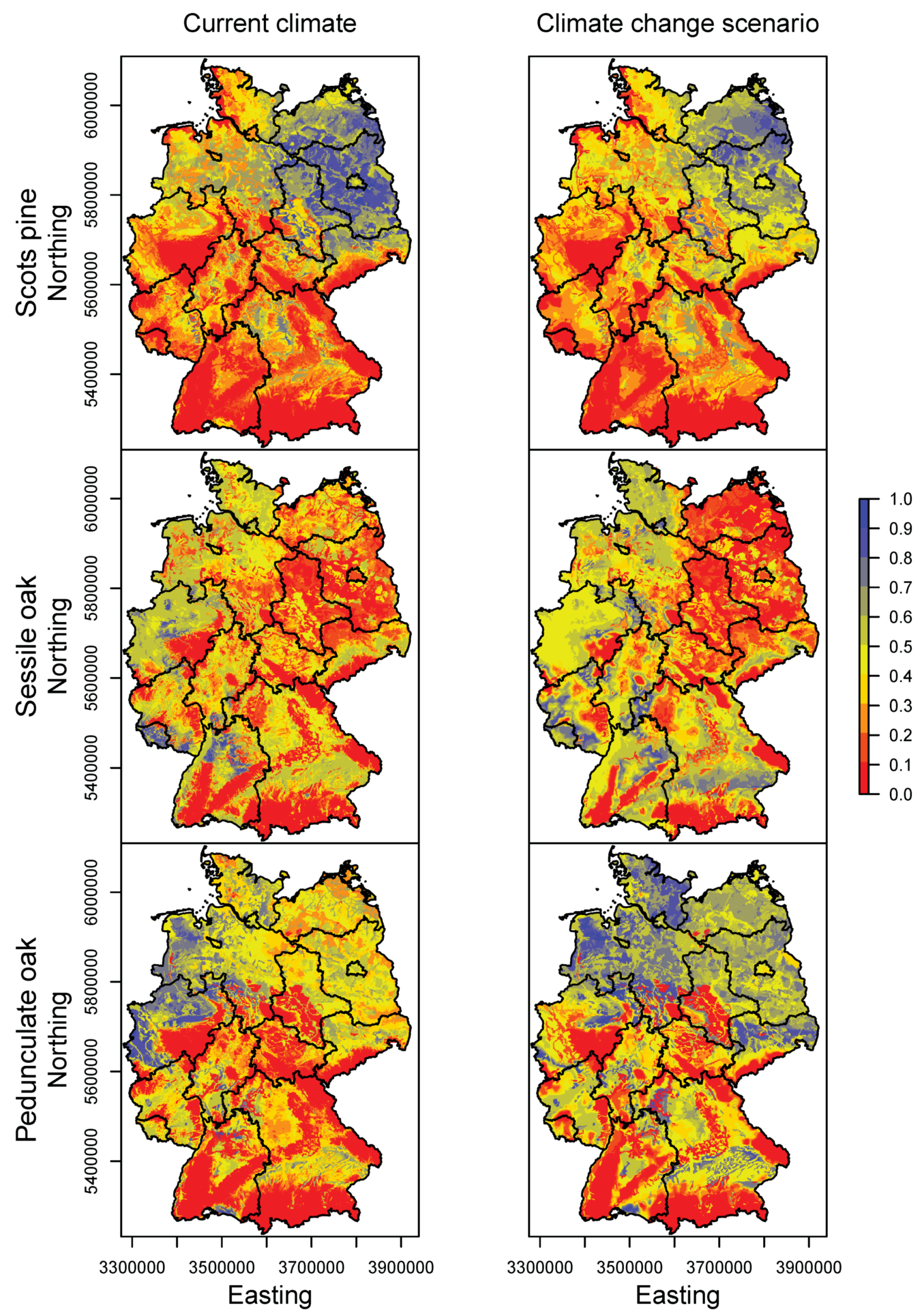
Figure 4.
Changes in the happy tree index under climate change for actual stands. The presence of species with species-specific high basal area share was considered. The maps show changes in site suitability for these species-specific occurrences within forests (according to Coordinated Information on the European Environment (CORINE) land cover data [39]). (EPSG code: 31467).

Figure 5.
Changes of site suitability between the current climate and climate change scenario until 2050 (RCP 8.5 [29]), separately displayed for distribution, growth, and happy tree index (HTI). Left bars represent forest area (according to Coordinated Information on the European Environment (CORINE) land cover data [39]) and right bars represent areas with species-specific high basal area share within forests (according to CORINE land cover). Minimal changes were defined as being smaller than the 5% quantile of all absolute values of changes.

Figure 6.
Priority regions for climate change adaptation in German forests derived from negative changes in happy tree index (HTI). The map shows priority classes for species-specific occurrences within forests (according to Coordinated Information on the European Environment (CORINE) land cover data [39]). Areas with high priority (highlighted in red) were considered priority regions for climate change adaptation. (EPSG code: 31467).

Figure 7.
Absolute area of priority classes within forests per federal state in km2. In determining priority classes, the expected negative change of site suitability and species-specific area were considered. High priority (highlighted in red) indicates priority regions for climate change adaptation. The bars are sorted in descending order according to the total summed area of the priority regions in the respective federal state.

Table 1.
Criteria used for variable selection. `-’ means that the best model was the standard model. DBH: Diameter at breast height. SBA: Slope-corrected stand basal area. AIC: Akaike information criterion. The × symbol stands for including a single spline for each temperature- and precipitation-related variable as well as their interaction term by using a two-dimensional spline.
| Species | Response | Model | Formula | Explained Deviance | AIC |
|---|---|---|---|---|---|
| Norway spruce | Species distribution | Best model | Mean temperature of coldest quarter × Annual precipitation + Soil | 23.23% | 3724.66 |
| Standard model | Annual mean temperature × Annual precipitation + Soil | 23.17% | 3747.68 | ||
| Growth | Best model | Standard model | - | - | |
| Standard model | Annual mean temperature × Annual precipitation + Soil + DBH + SBA | 54.58% | −5282.82 | ||
| European beech | Species distribution | Best model | Standard model | - | - |
| Standard model | Annual mean temperature × Annual precipitation + Soil | 8.25% | 4378.61 | ||
| Growth | Best model | Standard model | - | - | |
| Standard model | Annual mean temperature × Annual precipitation + Soil + DBH + SBA | 46.90% | −5403.11 | ||
| Scots pine | Species distribution | Best model | Standard model | - | - |
| Standard model | Annual mean temperature × Annual precipitation + Soil | 19.70% | 3717.81 | ||
| Growth | Best model | Standard model | - | - | |
| Standard model | Annual mean temperature × Annual precipitation + Soil + DBH + SBA | 54.46% | −5063.36 | ||
| Sessile oak | Species distribution | Best model | Annual mean temperature + Precipitation of warmest quarter + Soil | 18.58% | 2370.84 |
| Standard model | Annual mean temperature × Annual precipitation + Soil | 17.59% | 2386.42 | ||
| Growth | Best model | Standard model | - | - | |
| Standard model | Annual mean temperature × Annual precipitation + Soil + DBH + SBA | 47.50% | −2089.45 | ||
| Pedunculate oak | Species distribution | Best model | Mean temperature of coldest quarter + Precipitation of driest month + Soil | 9.97% | 4214.26 |
| Standard model | Annual mean temperature × Annual precipitation + Soil | 9.59% | 4220.1 | ||
| Growth | Best model | Standard model | - | - | |
| Standard model | Annual mean temperature × Annual precipitation + Soil + DBH + SBA | 50.48% | −2339.1 | ||
| Silver fir | Species distribution | Best model | Standard model | - | - |
| Standard model | Annual mean temperature × Annual precipitation + Soil | 31.17% | 929.97 | ||
| Growth | Best model | Standard model | - | - | |
| Standard model | Annual mean temperature × Annual precipitation + Soil + DBH + SBA | 54.36% | −650.27 |
Table 2.
Model quality of species distribution models and growth models. Growth models of sessile oak and pedunculate oak used only NFI2/3 data, because they were not identified at the species level in NFI 1. CV: coefficient of variation.
Table 2.
Model quality of species distribution models and growth models. Growth models of sessile oak and pedunculate oak used only NFI2/3 data, because they were not identified at the species level in NFI 1. CV: coefficient of variation.
| Species | Species Distribution | Growth |
|---|---|---|
| Pearson’s r2 (CV) | ||
| Norway spruce | 0.25 (0.023) | 0.38 (0.005) |
| European beech | 0.07 (0.045) | 0.23 (0.004) |
| Scots pine | 0.21 (0.032) | 0.37 (0.007) |
| Sessile oak | 0.08 (0.044) | 0.25 (0.009) |
| Pedunculate oak | 0.05 (0.055) | 0.31 (0.013) |
| Silver fir | 0.18 (0.049) | 0.34 (0.011) |
Table 3.
The proportion of happy tree index change per federal state between current conditions and the climate change scenario RCP 8.5 [29] until 2050 for each tree species. Change is displayed for the species-specific area within the forest area (according to Coordinated Information on the European Environment (CORINE) land cover data [39]). The three numbers indicate negative change/minimal change/positive change with minimal change being a 5% share of the smallest absolute change. City federal states were not displayed.
| Federal State | Norway Spruce | European Beech | Silver Fir | Scots Pine | Sessile Oak | Pedunculate Oak |
|---|---|---|---|---|---|---|
| Germany | 0.79/0.16/0.04 | 0.44/0.25/0.31 | 0.22/0.51/0.27 | 0.46/0.34/0.2 | 0.31/0.17/0.52 | 0.1/0.22/0.68 |
| Baden-Württemberg | 0.79/0.14/0.07 | 0.26/0.3/0.44 | 0.23/0.47/0.3 | 0.12/0.61/0.27 | 0.36/0.17/0.47 | 0.14/0.34/0.52 |
| Bavaria | 0.72/0.22/0.06 | 0.35/0.29/0.37 | 0.21/0.47/0.32 | 0.12/0.46/0.42 | 0.25/0.15/0.6 | 0.03/0.2/0.77 |
| Brandenburg | 0.52/0.48/0 | 0.93/0.07/0 | - | 0.86/0.13/0.01 | 0.43/0.31/0.26 | 0.01/0.08/0.91 |
| Hesse | 0.87/0.1/0.03 | 0.56/0.22/0.22 | - | 0.28/0.27/0.45 | 0.2/0.16/0.64 | 0.17/0.16/0.67 |
| Lower Saxony | 0.86/0.12/0.03 | 0.54/0.29/0.18 | - | 0.68/0.28/0.04 | 0.11/0.14/0.76 | 0.03/0.16/0.81 |
| Mecklenburg-West Pomerania | 0.9/0.1/0 | 0.9/0.1/0 | - | 0.32/0.5/0.18 | 0.91/0.06/0.03 | 0/0.15/0.85 |
| North Rhine-Westphalia | 0.83/0.14/0.03 | 0.25/0.29/0.46 | - | 0.24/0.65/0.11 | 0.18/0.21/0.6 | 0.38/0.31/0.31 |
| Rhineland-Palatinate | 0.78/0.18/0.04 | 0.43/0.26/0.32 | 0.15/0.8/0.05 | 0.2/0.54/0.26 | 0.29/0.15/0.56 | 0.15/0.3/0.55 |
| Saarland | 0.81/0.13/0.06 | 0.28/0.22/0.5 | - | 0.92/0.07/0.01 | 0.49/0.1/0.41 | 0.38/0.05/0.57 |
| Saxony-Anhalt | 0.89/0.1/0.01 | 0.55/0.2/0.25 | - | 0.84/0.16/0 | 0.5/0.25/0.25 | 0.02/0.17/0.8 |
| Saxony | 0.75/0.23/0.02 | 0.4/0.21/0.4 | - | 0.75/0.12/0.13 | 0.29/0.21/0.5 | 0/0.18/0.82 |
| Schleswig-Holstein | 0.94/0.06/0 | 0.67/0.3/0.03 | 0/1/0 | 0.32/0.59/0.09 | 0.2/0.12/0.68 | 0/0.18/0.82 |
| Thuringia | 0.83/0.14/0.03 | 0.48/0.2/0.32 | - | 0.04/0.24/0.71 | 0.42/0.22/0.36 | 0.01/0.2/0.79 |
© 2017 by the authors. Licensee MDPI, Basel, Switzerland. This article is an open access article distributed under the terms and conditions of the Creative Commons Attribution (CC BY) license (http://creativecommons.org/licenses/by/4.0/).
Share and Cite
MDPI and ACS Style
Märkel, U.; Dolos, K. Tree Species Site Suitability as a Combination of Occurrence Probability and Growth and Derivation of Priority Regions for Climate Change Adaptation. Forests 2017, 8, 181. https://doi.org/10.3390/f8060181
AMA Style
Märkel U, Dolos K. Tree Species Site Suitability as a Combination of Occurrence Probability and Growth and Derivation of Priority Regions for Climate Change Adaptation. Forests. 2017; 8(6):181. https://doi.org/10.3390/f8060181
Chicago/Turabian StyleMärkel, Ulrike, and Klara Dolos. 2017. "Tree Species Site Suitability as a Combination of Occurrence Probability and Growth and Derivation of Priority Regions for Climate Change Adaptation" Forests 8, no. 6: 181. https://doi.org/10.3390/f8060181
Note that from the first issue of 2016, this journal uses article numbers instead of page numbers. See further details here.