Article

Comparing Airborne Laser Scanning, and Image-Based Point Clouds by Semi-Global Matching and Enhanced Automatic Terrain Extraction to Estimate Forest Timber Volume

1
Chair of Remote Sensing and Landscape Information Systems, Institute of Forest Sciences, Faculty of Environment and Natural Resources, University of Freiburg, 79106 Freiburg, Germany
2
Forest Research Institute Baden-Württemberg (FVA), 79110 Freiburg, Germany
*
Author to whom correspondence should be addressed.
Forests 2017, 8(6), 215; https://doi.org/10.3390/f8060215
Submission received: 23 December 2016 / Revised: 8 June 2017 / Accepted: 15 June 2017 / Published: 17 June 2017
(This article belongs to the Special Issue Optimizing Forest Inventories with Remote Sensing Techniques)

Abstract

:
Information pertaining to forest timber volume is crucial for sustainable forest management. Remotely-sensed data have been incorporated into operational forest inventories to serve the need for ever more diverse and detailed forest statistics and to produce spatially explicit data products. In this study, data derived from airborne laser scanning and image-based point clouds were compared using three volume estimation methods to aid wall-to-wall mapping of forest timber volume. Estimates of forest height and tree density metrics derived from remotely-sensed data are used as explanatory variables, and forest timber volumes based on sample field plots are used as response variables. When compared to data derived from image-based point clouds, airborne laser scanning produced slightly more accurate estimates of timber volume, with a root mean square error (RMSE) of 26.3% using multiple linear regression. In comparison, RMSEs for volume estimates derived from image-based point clouds were 28.3% and 29.0%, respectively, using Semi-Global Matching and enhanced Automatic Terrain Extraction methods. Multiple linear regression was the best-performing parameter estimation method when compared to k-Nearest Neighbour and Support Vector Machine. In many countries, aerial imagery is acquired and updated on regular cycles of 1–5 years when compared to more costly, once-off airborne laser scanning surveys. This study demonstrates point clouds generated from such aerial imagery can be used to enhance the estimation of forest parameters at a stand and forest compartment level-scale using small area estimation methods while at the same time achieving sampling error reduction and improving accuracy at the forest enterprise-level scale.

1. Introduction

Accurate measurement and mapping of forest timber volume by affordable means is one of the primary objectives when designing forest inventories as an aid to forest management and operational harvesting activities. For a forest inventory, information on tree volume is vital. Given the fact that in large forest estates it is not practical to measure all the trees, the traditional approach in forest mensuration is the stand- or compartment-level inventory. In this approach, depending on the characteristics of a forest stand, full assessment, sampling inventory, stand-wise expert estimation, or a combination of different methods supported by the interpretation of aerial photography, are applied [1,2].
The concept of sample-based forest inventory for entire forest estates using statistical theory for parameter estimation was developed between 1960 and 1980 and is nowadays a widely-established system in forest management inventory practice, along with the traditional stand-wise approach which is still in use [3,4,5,6]. For forest estates that apply a sample-based forest inventory covering the entire forest area, e.g., several federal state forest enterprises in Germany, the combination of remote sensing with sample-based measurements offers a solution for wall-to-wall estimation.
With advances in the field of remote sensing in terms of availability and the quality of datasets, new methods integrating field reference data and remote sensing-based parameters have been developed and described, permitting the generation of forest timber volume maps [7,8,9]. These methods employ both parametric and non-parametric approaches where field information from forest inventories are combined with remote sensing information for the prediction and regionalization of forest timber volume estimates [7].
Many studies have highlighted the effectiveness of data from airborne laser scanning (ALS) for the estimation of above ground biomass and forest timber volume [8,9,10,11,12]. ALS has been used to derive precise and accurate information on forest structural characteristics [13] and in many Nordic countries, such as Norway, Finland, and Sweden, these data have been used operationally for forest inventory purposes [14,15,16]. However, given the relatively high cost of carrying out ALS surveys, the periodic update of data is limited as is its use in practice [17]. In contrast, stereo aerial photographs are acquired on a regular basis in a large number of countries. In many parts of Germany, for example, the survey administrations acquire stereo digital aerial photography on a three-year cycle [18].
The use of the spectral information from digital aerial photography is standard practice in forest resource surveys for mapping of forest types, structural attributes, etc. [19]. Further to recent developments in automatic image matching techniques, data derived from stereo aerial photographs, like ALS data, can now also be used for generation of three-dimensional point clouds which can then be applied using different approaches to estimate forest timber volume. The objective of this study is to explore how these ALS and aerial image point cloud data can be used in conjunction with sample-based forest inventory data to provide spatially-explicit timber volume maps.
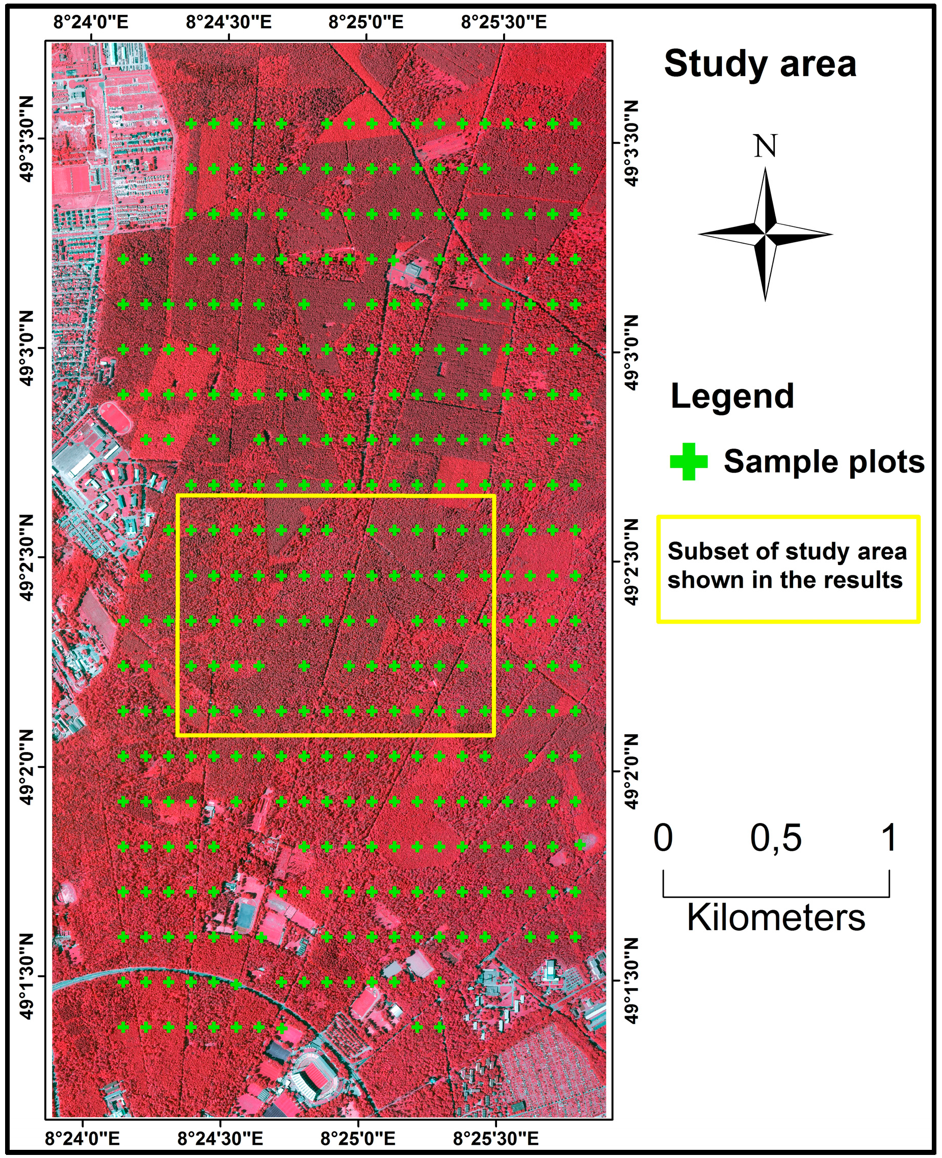
The pixel resolution of stereo aerial images from administration surveys is usually relatively high (10-cm pixel size in our study where we use standard images from the survey agency of the federal state of Baden-Württemberg) and offers a good potential for extracting dense three-dimensional image-based point clouds [20]. On the other hand, ALS point clouds obtained from laser pulses are more uniformly distributed than image-based point clouds [21].
For the extraction of canopy height information from image-based point clouds, a high-quality digital terrain model, based on ALS data is required [20,21]. For all German federal states in general, and at our study site in particular, highly accurate digital terrain models from earlier ALS campaigns are available.
Over the last few years, different image-matching point cloud-generating algorithms have been developed and tested for the estimation of different forest attributes. For instance, Bohlin et al. [22] used Match-T DSM software to generate point clouds for estimation of forest attributes. Similarly, White et al. [23] used the Semi-Global Matching (SGM) algorithm as implemented in the Remote Sensing Software Package Graz [24] to generate point clouds for estimating plot-level forest attributes. Järnstedt et al. [25] used the Next-Generation Automatic Terrain Extraction module from the software SOCET SET, and Straub et al. [21] used enhanced Automatic Terrain Extraction (eATE) algorithm from the IMAGINE Photogrammetry software of ERDAS IMAGINE, for the estimation of forest attributes.
For our study, two of the most widely-used image-matching point cloud-generating algorithms, namely the eATE and SGM have been selected. The eATE algorithm is an area-based method and uses a normalized cross correlation strategy [26] while SGM, which is also an area-based method, considers semi-global cost functions during the matching process [27]. While many studies have opted to use SGM among the various image-matching algorithms [28,29,30], so far no study has specifically focused on comparing the ability of image-matching algorithms to produce accurate point clouds over forests and to compare those point clouds generated with point clouds obtained using high-quality ALS.
Although height, obtained from ALS or image-based point clouds, is an important variable used to model forest timber volumes, other parameters derived from point clouds (density and height metrics) have been observed to further improve the performance of such models. While many studies exist where the relationship between forest timber volume and different remote sensing parameters has been statistically modelled using parametric and non-parametric modelling approaches, a comprehensive evaluation of forest timber volume modelling approaches for different image-matching point clouds and their performance against approaches using ALS point clouds, is missing. Existing modelling examples include the approaches of Latifi et al. [8], who used non-parametric methods for estimating forest timber volume and biomass in a temperate forest using ALS data, and Rahlf et al. [31], who adopted parametric multiple linear regression for estimating forest timber volume.
In addition to comparing the ALS and image-based point clouds in this study, we also test the relative performance of models based on parametric multiple linear regression, and non-parametric k-Nearest Neighbour (k-NN) and Support Vector Machine (SVM) for the assessment and mapping of forest timber volume using the height and density metrics. To summarise, the specific objectives of the present study are to (i) assess the use and potential of image-matching SGM and eATE image-based point clouds for wall-to-wall mapping of forest timber volume in comparision to wall-to-wall mapping of timber volume using ALS data, and (ii) compare the performance of parametric multiple linear regression, non-parametric k-NN and SVM for the assessment of forest timber volume using ALS and image-matching point clouds.

2. Material and Methods

2.1. Study Site and Field Sample Plots

The study site, 120 m above sea level, is located in the federal state of Baden-Württemberg, Germany, towards the north of Karlsruhe and extends from 49°3′37.302′′ N and 8°24′2.846′′ E to 49°01′18.773′′ N and 08°25′49.981′′ E (Figure 1). The total size of the study area is approximately 12 km2 and the dominant tree species are Scots pine (Pinus sylvestris L.) (56.3%), European/Common beech (Fagus sylvatica L.) (17.8%), Sessile oak (Quercus petraea leibel.) and Red oak (Quercus rubra L.) (Jointly 14.9%). Other tree species, including Douglas fir (Pseudotsuga menziesii), Norway spruce (Picea abies) and European larch (Larix decidua) also occur occasionally. Structurally, the forest is multi-layered, although predominantly the strata are two-layered dense forests. The forest type is temperate and not typical of the average conditions in Baden-Württemberg where spruce is the dominant species.
Field data were collected through a forest inventory carried out by the state forest service of Baden-Württemberg in summer 2007 where tree measurements were recorded from 375 permanent sample plots (Figure 1). The sample plots, each measuring 12 m in diameter, are distributed systematically over the study area in a 100 m × 200 m grid. For each plot, trees were sampled in concentric circles originating from the centre of the plot in such a way that trees with diameter at breast height (dbh) smaller than 7 cm are sampled only up to a radius of 2 m; trees between 7 cm and 15 cm are measured within a radius of 3 m; trees between 15 cm and 30 cm are measured up to 6 m distance; and trees with dbh over 30 cm are measured up to the maximum distance of 12 m radius. Two dominant heights of each main tree species and one dominant height of other mixed species were measured. The remaining tree heights were predicted by species-specific stand height curves developed by the Forest Research Institute, Baden-Württemberg, Germany. The single tree timber volume was calculated using the taper functions of Kublin [32], and the total volume at plot-level in cubic meters per hectare was derived by summing up the individual tree volumes weighted by the inverse of the corresponding sample plot area (Table 1). More detail about the methodology can also be found in Latifi et al. [8]. Figure 2 shows the distribution of the age classes, ranging from 10–160 years, for trees in all sample plots in the study area.

2.2. Remote Sensing Data

ALS data used in this study were acquired by Milan Geo service GmbH using the IGL Litemapper 5600 system with a Riegl LMS-Q560 (240 kHz) scanner in early November 2009. The details of the flight and system parameters of ALS campaigns are shown in Table 2.
The stereo aerial photographs were provided by the Forest Research Institute of Baden-Württemberg, Germany. A block of 28 stereo images were acquired in August 2009 using an UltraCamXP frame camera enabled to capture four spectral bands corresponding to the wavelengths of blue, red, green and near-infrared channels. The images have a ground resolution of 0.1 m, and the along-track and across-track overlap is 60% and 30%, respectively. The flying altitude of the aircraft was 2950 m above sea level, and the orientation was carried out by initial measurements using the global navigation satellite system and inertial measurement unit. The aero-triangulation was achieved with ground control points received from the survey agency of the federal state of Baden-Württemberg, Germany.

2.3. Image Matching

Image-based point clouds were generated from stereo aerial photographs by using eATE manager and SGM (integrated module in IMAGINE Photogrammetry software package of ERDAS IMAGINE). eATE is an area-based approach (moving window) for the identification of correspondence pixels along the epipolar line, using a normalized cross-correlation matrix between the left and right overlapping images [33,34]. SGM was developed by Hirschmüller [27,29,35] and is a hybrid global- and area-based approach utilizing radiometric robust mutual information and a smoothness constraint to generate dense surface point clouds. The approach first identifies a pixel on the base image and then searches for the similar pixel along the epipolar line in the paired image. The minimum aggregated cost leads to a disparity map. Both image-matching algorithms require the selection of input parameters. We tested many different parameter combinations to identify the best-performing parameters. The final selected ones are shown in Table 3.
The detailed explanation of all strategy settings for the parameters used in eATE and SGM can be found in ERDAS IMAGINE [33] and Ullah et al. [34].

2.4. Computation of Explanatory Variables

The point clouds derived from stereo aerial photographs using both the image-matching algorithms and the ALS point clouds were normalized to the height above ground surface by using the difference between the point heights and the corresponding pixel heights from ALS-based digital terrain model at a spatial resolution of 1 m. The different height-related metrics were extracted from the normalized image-based and ALS point clouds falling within the 12 m radius circular sample plot areas. Further descriptions about these metrics have been provided in Table 4.
In addition to height metrics, we also extracted canopy cover density metrics for each sample plot from 1 m resolution canopy height models which were generated by subtracting ALS-based digital terrain model from the three digital surface models interpolated from SGM based-, eATE based- and ALS-based point cloud data. The digital surface models and digital terrain model were generated using TreesVis software [36], which takes the highest point for the digital surface model and lowest point for digital terrain model within pre-specified pixel resolution. For interpolation, the algorithm employs the general technique of matching a deformable surface to the point clouds by using energy minimization. Details of the methodological approach for the generation of digital terrain and surface models can be found in Weinacker et al. [37].
To generate canopy cover density metrics, we adopted the approach proposed by Jennings et al. [38] and used by Rahlf et al. [31] and Straub et al. [21]. Ten canopy cover density metrics were calculated as shown in Table 4 and the canopy cover was estimated as the proportion of ground presumably covered by tree crowns. For each sample plot, the range between the minimum (>2 m) and maximum canopy height was divided into ten equal lengths with the boundary between two adjacent fractions forming the threshold which was then used to separate the relevant tree crown regions. The potential crown region corresponding to a fraction was identified by selecting all those pixels from the canopy height model which were above a certain threshold. A ratio of the sum of number of pixels corresponding to crown region above the different thresholds (heights) to the total numbers of pixels per sample plot was used as an estimate for the canopy cover density. Additionally, canopy cover density was calculated by dividing the sum of the number of pixels in vertical height above 2 m by the total number of pixels falling within the 12 m radius of circular sample plots. As a final step, the sum of heights of all 1 m × 1 m pixels within each sample plot was calculated.
The importance of all the above height metrics for the prediction of forest attributes has been explained in detail by Bohlin et al. [22], Rahlf et al. [31] and Straub et al. [21].

2.5. Modelling and Mapping

A total of 27 parameters (i.e., 16 height- and 11 density-related metrics) were extracted from the normalized point clouds and canopy height models which were used as explanatory variables during the development of models for forest timber volume estimation (Table 4). The first step was to exclude any multicollinearity observed in the form of high degree of correlation (>0.7) between some of the explanatory variables. The decision to drop the variables was taken by using the variance inflation factor which provides a robust quantification of the severity of multicollinearity. The CAR package of R-statistics software [39] and the method described by Zuur et al. [40] were used to fit multiple linear regression models with all explanatory variables and then observing the variance inflation factors for each of the variables. The variables were dropped when the variance inflation factor exceeded a value of 2.0. The absence of any remaining collinearity was confirmed by screening pairwise plots and the correlation coefficient for pairs of variables.
The explanatory variables remaining after exclusion of collinearity were used for fitting multiple linear regression models with forest timber volume measured per plot as the response variable. Out of the remaining variables, the least significant ones were dropped out at every step and the model refitted iteratively until dropping a variable did not result in further lowering of the model’s Akaike Information Criterion. The explanatory variables remaining at the last step formed the final set which were then used for k-NN, SVM and multiple linear regression-based modelling of forest timber volume at the plot-level.
k-NN is a well-known non-parametric method for estimating forest timber volume and has been operationally used in the Finnish national forest inventory since 1990 [41]. Its advantage is the simplicity of its algorithm and its general applicability independent of the character of the relationship between the target and explanatory variables provided that the number of terrestrial samples is large. The same set of explanatory variables as used for the multiple linear regression were used in the k-NN without using any additional weighting. Similarity measure used to identify the k “nearest” data points was the Euclidean distance. It is the most commonly-used distance in the k-NN computation and is also the best proximity measure. The k-NN procedure starts by using k = 5 (taking the average of 5 nearest neighbours), which is the default for the caret package in the R platform [42], and calculates the Euclidean distance. Then it tests k = 7 and k = 9 and further increases the tune length to k = 11, k = 13 and so on. The objective of this approach is to identify a suitable k-value which corresponds with the lowest root mean square error (RMSE) between the predicted and the observed values. In our case, the final k-value of 9 was used for all of the three datasets.
SVM is also a non-parametric method primarily used for the classification of hyperspectral and multispectral data [43,44,45], but has also been used for regression analysis [46]. It separates the classes with a decision surface by maximizing the margin between the classes [47]. For the linear case, the surface is called the optimal hyperplane. It leaves the maximum margin between the two classes, and the data points closest to the surface are called the support vectors [48]. The support vectors are the critical elements of the training sets. The optimal surface solution is achieved by applying different kernel functions like linear, polynomial and radial. We tested all the kernel functions as implemented in R caret package [42] and the most accurate results (i.e., lowest RMSE) were obtained by using a linear kernel function. For SVM also the same set of explanatory variables, as used for multiple linear regression and k-NN, was used.
The accuracy assessment was done using RMSE and bias%. To determine the prediction accuracy, the absolute and relative RMSE (Equations (1) and (2)) were computed by using leave-one-out cross validation, where each single observation was held out as a testing set, and the remaining data were used as a training set. The caret package of R-statistical software [42,49] was used for the statistical analysis.
R M S E   [ m ] = 1 n i = 1 n ( y i y i ^ ) ²
R M S E   [ % ] = R M S E   ( L O O C V ) y × 100
where y i is the observed values, y ^ i is the predicted value of leave-one-out cross validation, y is the mean of the observed values and n is the total number of ground sample plots.
For the calculation of bias%, we used the “hydroGOF” package of R-statistics software [50].
Bias% = 100 × [sum (predicted − observation)/sum (observation)]
Finally, the models were used to produce wall-to-wall forest timber volume maps by implementing the prediction algorithms developed by the three modelling approaches on the rasterized explanatory variables. A pixel resolution of 20 m was used for mapping, which is considered to be a suitable mapping unit for 12 m radius circular ground sample plots, as described by White et al. [51] in best practice guidelines for generating forest inventory attributes from ALS data using an area-based approach.

3. Results

The comparison of multiple linear regression models for ALS-based and image-based point clouds (Table 5) shows that the performance of ALS for modelling forest timber volume was the highest. However, the coefficient of determination (R2) and adjusted R2 values for SGM were marginally lower than those from ALS at 1%. The eATE-based point clouds were found to be the dataset which showed the lowest performance in terms of R2 and adjusted R2 among the three datasets in this comparison.
The results of the comparison of methods for estimating the forest timber volume show that, irrespective of the origin of point clouds, multiple linear regression models showed slightly higher accuracies compared to k-NN and SVM, which can also be observed in the RMSE and RMSE% in Table 6. The bias% for multiple linear regression models for all three types of point clouds was minuscule, while with 
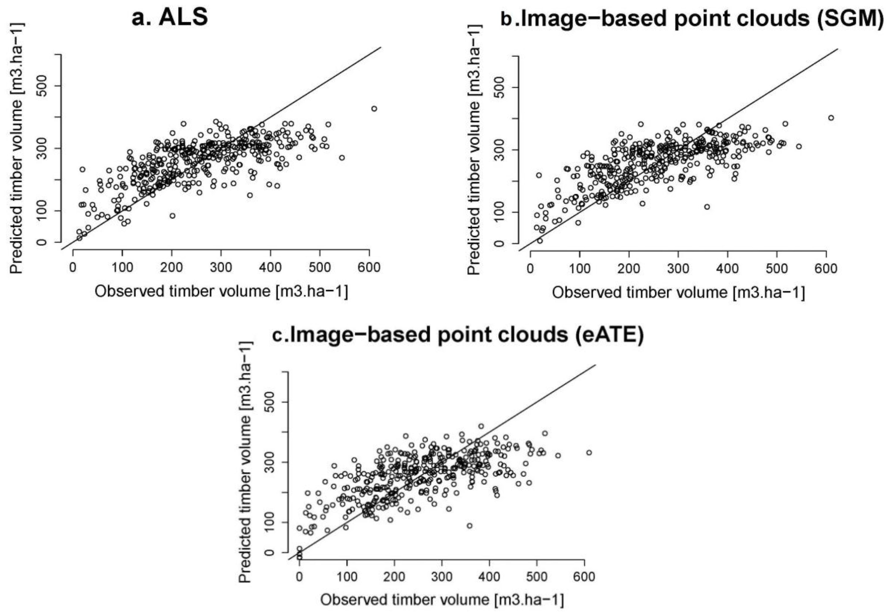
k-NN and SVM small positive and negative biases were observed respectively. There is also a tendency to overestimate forest timber volume for the lower ranges and underestimate at the higher ranges as shown in Figure 3 where the goodness of fit between predicted and measured forest timber volumes has been plotted.
Table 6 further shows that for all the three forest timber volume estimation approaches, the best results, i.e., the lowest RMSE, RMSE% and bias% were obtained by using the ALS-based point clouds. Among the image-matching point clouds, the SGM point clouds produced better results for all the three approaches while eATE point clouds showed the overall least performance which is consistent with the earlier observations, whereas the best fit using the eATE point clouds was still significantly lower than those obtained using SGM and ALS point clouds (Table 5).
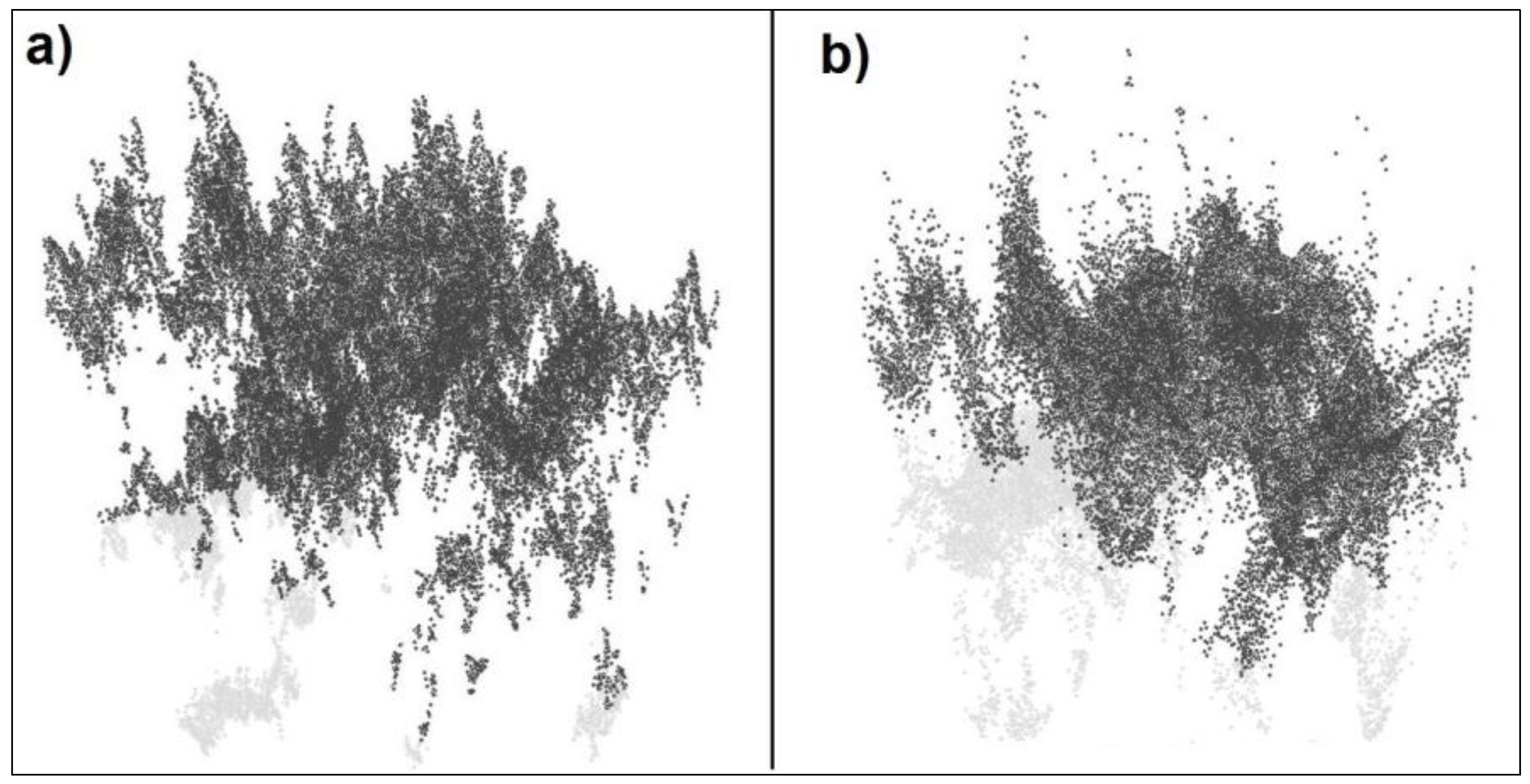
The higher performance of SGM-based point clouds compared to eATE, is an indication of the method’s ability to capture the three-dimensional structure of trees better than those from eATE. This feature of SGM is also represented in Figure 4 where a visual comparison of the vertical profile of point clouds for the small subset area is shown. These show that image-based points obtained using SGM are denser and have better coverage of the trees tops and the surrounding crowns than eATE image-based point clouds.
The relative performance of the two image-matching algorithms, in terms of density of point clouds (points per m2) and their ability to obtain true matches for existing trees, is further highlighted in Figure 5 where image-based point cloud densities from SGM and eATE algorithms for a subset of the study area are compared. For SGM, a mean point density of 27.66 m2 was calculated. This value is significantly higher when compared to a mean density of 3.29 m2 for eATE point clouds. Similarly, it was observed that eATE produced considerably higher numbers of no data pixels, thereby suggesting a higher rate of failure in obtaining valid data points during the image matching procedure. Conversely, for SGM, very few pixels with no data in the point clouds were observed.
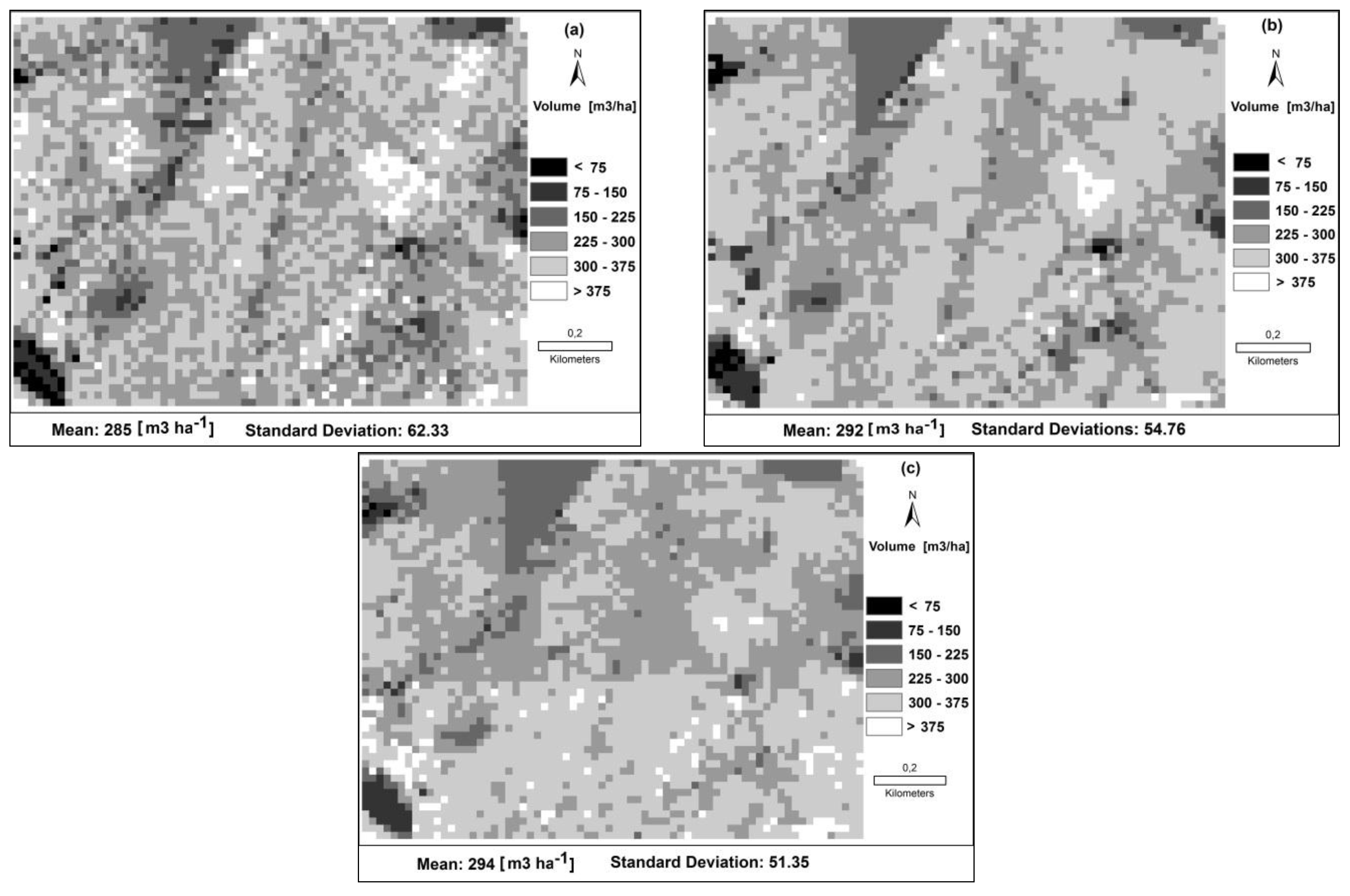
Finally, Figure 6 shows the thematic maps generated for forest timber volume focused on a small subset of the total study area. The estimations shown here are based on the models developed using multiple linear regression approaches. For this subset study area, we observed a mean forest timber volume of 285 (m3 ha−1) for ALS point clouds, a volume which is slightly lower than image-based point clouds based on SGM (292 m3 ha−1) and eATE (294 m3 ha−1) respectively.

4. Discussion

The first objective of our study was to assess the accuracy of image-matching SGM and eATE image-based point clouds in comparsion with ALS for wall-to-wall mapping of forest timber volume. For our test site, we obtained a RMSE% of 28.3 using SGM image matching, 29.0 when using eATE image matching and 26.3 for ALS. A review of comparable studies in the literature shows the results can vary based on stand structure, species and site quality. For example, Rahlf et al. [31] analyzed the potential of ALS versus image-based point clouds for estimating forest timber volume, but used the Next-Generation Automatic Terrain Extraction image-matching algorithm as implemented in SOCET SET (version 5.5) at a spruce-dominated test site in southern Norway. They found a higher RMSE% difference between ALS and image-based point clouds and the ALS performing much better, with a RMSE% of 19.0, compared to 31.0, when using an image-based point cloud. White et al. [23] also tested ALS in comparison with image-based point clouds, and used SGM implemented in the Remote Sensing Software Package Graz (Version 7.46.11) for plot-level estimation of Lorey’s height, basal area, and forest timber volume in a complex coastal forest environment in Canada. They obtained a RMSE% of 33.2 for ALS and a relatively closer result of 36.9% RMSE for SGM. Järnstedt et al. [25] compared ALS with image-based point clouds by using the Next-Generation Automatic Terrain Extraction module from the software SOCET SET for estimation of mean diameter, basal area, mean and dominant height and forest timber volume for a test site in Southern Finland. Like Rahlf et al. [31], they also found a higher RMSE% difference between ALS and image-based point clouds and the ALS performed much better with a RMSE% of 31.3 compared to 40.4 when using the image-based point cloud.
Summarizing our results and looking at the findings of above studies, we can conclude that in general, image-based point clouds using SGM show, in most but not in all cases, comparable results to ALS. Furthermore, in all cases, the achievable RMSE% variation from the test site to test site is relatively close and small, demonstrating the operational potential of image-based point clouds for wall-to-wall mapping of forest volume.
When comparing the performance of SGM and eATE in our study, we obtained poorer results using eATE. The observed differences are due to the entirely different matching and filtering algorithms. They also differ in the sensitivity of the surface direction and the contrast changes within objects. Additionally, SGM has been developed to produce a closed surface, while eATE concentrates on matching processes without producing regular gridded closed surfaces. As discussed earlier, SGM uses a semi-global cost function, which considers an approximation of the global cost and explicit smoothness constraints. On the other hand, eATE uses an area-based approach without taking into account cost functions. Unlike ALS, SGM produces a more evenly distributed point cloud corresponding to the ground sample distance of the imagery, which is spread over the entire forest area when compared to eATE (Figure 4 and Figure 5). However, eATE produces an unevenly distributed point cloud when compared to SGM, which is in some areas successful but fails in other regions completely, due to the inadequate texture or occlusion in parts in the images (Figure 5). For this reason, we found a large number of pixels with no data values for eATE, as compared to SGM (Figure 5). For SGM, we obtained a mean point cloud density of 27.7 m2, which is much higher as compared to 3.3 m2 obtained from eATE (Figure 5). In terms of computational power requirements, SGM needs less processing time compared to eATE for the generation of image-based point clouds. SGM needs very few parameters settings (Table 3), while eATE needs many parameters to be set by the operator and therefore needs more user input and model iterations to identify the appropriate parameter set for a specific image dataset. Hence, there are many reasons for obtaining a higher accuracy by using SGM as compared to eATE. Straub et al. [21] also highlighted the problem of the no data points when using eATE for estimating forest timber volume and basal area and they have suggested exploring SGM as a potential solution. The results of our comparison of SGM and eATE for forest timber volume estimation are also supported by our previous findings on the comparison of these two methods for forest height estimation [34].
When comparing the performance of parametric multiple linear regression and non-parametric k-NN and SVM for estimating forest timber volume, we achieved slightly more accurate results using a parametric multiple linear regression, specifically when considering the bias. However, multiple linear regressions did not substantially outperform the other two non-parametric k-NN and SVM approaches. Penner et al. [52] worked on the comparison of parametric versus non-parametric ALS models for operational forest inventory in boreal Ontario. They implemented and compared seemingly unrelated regression models (parametric), k-NN and randomForest (non-parametric) predictions of forest inventory attributes. They found, similar to the results presented in this study, that no single method produces the best results consistently, and that the prediction accuracy varied markedly with the forest type.
We observed an overestimation of forest timber volume at the lower ranges and underestimation at the higher ranges (Figure 3). This could be due to the presence of older trees which show increased height increment relative to diameter increment when compared to younger trees [53], and due to the fact that tree height was used as one of the explanatory variables for forest timber volume estimation. The overestimation could also be due to overlapping tree crowns located outside of the borders of the sample plots. This would appear to be one of the limitations when integrating forest inventory field survey data with remote sensing datasets, using an area-based approach. However, this phenomenon also works in reverse, as some crowns on the edge of the plot are only partially included. Therefore statistically, these phenomena should neutralize each other.
Our maps showed a mean forest timber volume of 285 [m3 ha−1] for ALS for the small subset area, which is slightly lower than image-based point clouds using SGM [i.e., 292 m3 ha−1] and eATE [i.e., 294 m3 ha−1] (see Figure 6). We found that all three datasets produce more or less comparable results. There is a slight overestimation in forest timber volume maps from image-based point clouds compared to ALS. This could be attributed to the penetrating power of the ALS point clouds as compared to the image-based point clouds. For the eATE-based point clouds, there is a clear difference between the forest timber volume maps in areas where highest and lowest point densities are present. The standard deviation of each of the maps also highlights the ability of ALS to capture the structural diversity of the forests compared to the image-based point clouds.

5. Conclusions

In this study we assessed the use and potential of image-matching SGM and eATE image-based point clouds to aid wall-to-wall mapping of forest timber volume in comparison to wall-to-wall mapping of forest timber volume using ALS data. The performance of a parametric multiple linear regression model and the non-parametric k-NN and SVM methods were evaluated for the estimation of forest timber volume.
ALS data, independent of the parameter estimation method used, provided slightly more accurate volume estimates than image-based point clouds from SGM and eATE. Nevertheless, image-based point clouds provide maps of comparable quality to ALS and can thus be used in a forest management planning context where ALS data are absent but where recent aerial images and sample field plot data are readily available. With respect to the methods applied in this study for image matching, SGM slightly outperformed eATE while the timber volume predictions generated using multiple linear regression showed slightly better results compared to k-NN and SVM.
The results from this study show how remotely-sensed data from aerial imagery and ALS can be combined with plot-based data to improve estimates of the most meaningful forest inventory parameters and to generate information layers or thematic map products to aid forest management. Besides using such maps as a general information layer for decision support, there is also a significant potential to combine these data with sample plot information through small area estimation to provide improved estimation accuracy at the stand, compartment and forest enterprise level scales.

Acknowledgments

The authors are most thankful to Shaheed Benazir Bhutto University, Sheringal Dir Upper and Higher Education Commission of Pakistan for awarding Sami Ullah a Ph.D. scholarship, which enabled this research. Furthermore, we are thankful to the European Commission for the financial support for the project: Delivery of sustainable supply of non-food biomass to support a “resource-efficient” Bioeconomy in Europe (S2BIOM). This research is closely linked with and was partly funded by S2Biom, which is co-funded by the European Commission in the 7th Framework Programme (Project No. FP7-608622, Project website: http: //www.s2biom.eu/en/). The authors are also grateful to Gerald Kändler, Forest Research Institute, Baden-Württemberg (FVA), Germany, for the provision of stereo aerial photographs, field inventory data and related processing support at FVA. The article processing charge was funded by the German Research Foundation (DFG) and the University of Freiburg in the funding programme Open Access Publishing.

Author Contributions

Sami Ullah is the lead author and was involved in the overall processing, analysis, and writing. Petra Adler supported the processing of the stereo aerial photographs. Matthias Dees designed the experiment. Pawan Datta contributed to the implementation of the methodological approach. The first draft of the manuscript was prepared by Sami Ullah and was further improved by Matthias Dees, Petra Adler, Pawan Datta, and finally by Barbara Koch.

Conflicts of Interest

The authors declare no conflict of interest.

References and Notes

  1. Federal State Forest Service of Baden-Württemberg. Instructions for Forest Management Planning to be Applied by the Federal State Forest Service of Baden-Württemberg; Federal State Forest Service of Baden-Württemberg: Freiburg Germany, 2002. [Google Scholar]
  2. Dees, M. Kombination von Fernerkundung und Stichprobeninventur bei Betrieblichen und Nationalen Waldinventuren (Combination of Remote Sensing and Sample Based Observation for Operational and National Forest Incentives); University of Freiburg: Freiburg, Germany, 2006. [Google Scholar]
  3. Kändler, G.; Bösch, B. Die Betriebsinventur als Grundlage für Planung, Steuerung und Kontrolle des Forstbetriebs (Forest enterprise inventory for planning and control of a forest enterprise). Wissenstransfer in Praxis und Gesellschaft FVA-Forschungstage 2001, 18, 252–265. [Google Scholar]
  4. Schmid-Haas, P. Stichprobenerhebungen. Begründungen zu den Aufnahmeinstruktionen (Sampling Assessments. Justifications on the Inventory Instructions); Birmensdorf, Eidgenössische Forschungsanstalt für Wald, Schnee und Landschaft: Birmensdorf, Switzerland, 1964; 8p. [Google Scholar]
  5. Schmid-Haas, P.; Werner, J.; Baumann, E. Forest Inventories by Unmarked Permanent Sample Plots; Swiss Federal Institute for Forest, Snow and Landscape Research: Birmensdorf, Switzerland, 1978; 135p. [Google Scholar]
  6. Schöpfer, W.; Stiefvater, H. Stand und Entwicklung der Betriebsinventur in der Bundesrepublik Deutschland (Status and development of permanent forest inventories in Germany). Die Verfahren der Bundesländer im Vergleich (A comparison of the approaches used by federal states). In Arbeitskreis Zustandserfassung und Planung in der AG Forsteinrichtung: Stand und Entwicklung der Betriebsinventur auf Stichprobenbasis in der BRD; Dokumentationsband der FVA Baden-Württemberg: Freiburg, Germany, 1990; pp. 10–60. [Google Scholar]
  7. Hill, A.; Breschan, J.; Mandallaz, D. Accuracy assessment of timber volume maps using forest inventory data and LiDAR canopy height models. Forests 2014, 5, 2253–2275. [Google Scholar] [CrossRef]
  8. Latifi, H.; Nothdurft, A.; Koch, B. Non-parametric prediction and mapping of standing timber volume and biomass in a temperate forest: Application of multiple optical/LiDAR -derived predictors. Forestry 2010, 83, 395–407. [Google Scholar] [CrossRef]
  9. Maack, J.; Lingenfelder, M.; Weinacker, H.; Koch, B. Modelling the standing timber volume of Baden-Württemberg—A large-scale approach using a fusion of Landsat, airborne LiDAR and national forest inventory data. Int. J. Appl. Earth Obs. Geoinf. 2016, 49, 107–116. [Google Scholar] [CrossRef]
  10. Hollaus, M.; Wagner, W.; Maier, B.; Schadauer, K. Airborne laser scanning of forest stem volume in a mountainous environment. Sensors 2007, 7, 1559–1577. [Google Scholar] [CrossRef]
  11. Kankare, V.; Vastaranta, M.; Holopainen, M.; Räty, M.; Yu, X.; Hyyppä, J.; Hyyppä, H.; Alho, P.; Viitala, R. Retrieval of forest aboveground biomass and stem volume with airborne scanning LiDAR. Remote Sens. 2013, 5, 2257–2274. [Google Scholar] [CrossRef]
  12. Sheridan, R.D.; Popescu, S.C.; Gatziolis, D.; Morgan, C.L.; Ku, N.-W. Modeling forest aboveground biomass and volume using airborne LiDAR metrics and forest inventory and analysis data in the Pacific Northwest. Remote Sens. 2014, 7, 229–255. [Google Scholar] [CrossRef]
  13. Maltamo, M.; Næsset, E.; Vauhkonen, J. Forestry applications of airborne laser scanning. Concepts Case Stud. Manag. Ecosyst. 2014, 27, 2014. [Google Scholar]
  14. Maltamo, M.; Packalen, P. Species-specific management inventory in Finland. In Forestry Applications of Airborne Laser Scanning; Springer: Berlin, Germany, 2014; pp. 241–252. [Google Scholar]
  15. Næsset, E. Airborne laser scanning as a method in operational forest inventory: Status of accuracy assessments accomplished in Scandinavia. Scand. J. For. Res. 2007, 22, 433–442. [Google Scholar] [CrossRef]
  16. Næsset, E. Area-based inventory in Norway-from innovation to an operational reality. In Forestry Applications of Airborne Laser Scanning; Springer: Berlin, Germany, 2014; pp. 215–240. [Google Scholar]
  17. Dees, M.; Straub, C.; Koch, B. Can biodiversity study benefit from information on the vertical structure of forests? Utility of LiDAR remote sensing. Curr. Sci. 2012, 102, 1181–1187. [Google Scholar]
  18. Ullah, S.; Adler, P.; Dees, M.; Koch, B. Evaluating the potential of stereo aerial photographs for canopy height model generation. Forstli. Forsch. 2015, 214, 83–90. [Google Scholar]
  19. Hildebrandt, G. Fernerkundung und Luftbildmessung für Forstwirtschaft, Vegetationskartierung und Landschaftsökologie (Remote Sensing and Photogrammetry for Forestry, Vegetation Mapping and Landscape Ecology); Wichmannn: Heidelberg, Germany, 1996; p. 675. [Google Scholar]
  20. White, J.C.; Wulder, M.A.; Vastaranta, M.; Coops, N.C.; Pitt, D.; Woods, M. The utility of image-based point clouds for forest inventory: A comparison with airborne laser scanning. Forests 2013, 4, 518–536. [Google Scholar] [CrossRef]
  21. Straub, C.; Stepper, C.; Seitz, R.; Waser, L.T. Potential of UltraCamX stereo images for estimating timber volume and basal area at the plot level in mixed European forests. Can. J. For. Res. 2013, 43, 731–741. [Google Scholar] [CrossRef]
  22. Bohlin, J.; Wallerman, J.; Fransson, J.E. Forest variable estimation using photogrammetric matching of digital aerial images in combination with a high-resolution DEM. Scan. J. For. Res. 2012, 27, 692–699. [Google Scholar] [CrossRef]
  23. White, J.C.; Stepper, C.; Tompalski, P.; Coops, N.C.; Wulder, M.A. Comparing ALS and image-based point cloud metrics and modelled forest inventory attributes in a complex coastal forest environment. Forests 2015, 6, 3704–3732. [Google Scholar] [CrossRef]
  24. Joanneum Research. Remote Sensing Graz; Version 7.46.11.; Joanneum Research: Graz, Austria, 2015. [Google Scholar]
  25. Järnstedt, J.; Pekkarinen, A.; Tuominen, S.; Ginzler, C.; Holopainen, M.; Viitala, R. Forest variable estimation using a high-resolution digital surface model. ISPRS J. Photogramm. Remote Sens. 2012, 74, 78–84. [Google Scholar] [CrossRef]
  26. ERDAS IMAGINE Help Erdas imagine. Online help for Erdas imagine delivered with Erdas Imagine 2015, HEXAGON GEOSPTIAL. 2014.
  27. Hirschmüller, H. Stereo processing by semi-global matching and mutual information. IEEE Trans. Pattern Anal. Mach. Intell. 2008, 30, 328–341. [Google Scholar] [CrossRef] [PubMed]
  28. Gehrke, S.; Morin, K.; Downey, M.; Boehrer, N.; Fuchs, T. Semi-Global Matching: An alternative to LiDAR for DSM generation. In Proceedings of the 2010 Canadian Geomatics Conference and Symposium of Commission I, Calgary, Canada, 15–18 June 2010. [Google Scholar]
  29. Hirschmuller, H. Accurate and efficient stereo processing by semi-global matching and mutual information. In Proceedings of the 2005 IEEE Computer Society Conference on Computer Vision and Pattern Recognition (CVPR 2005), San Diego, CA, USA, 20–25 June 2005; pp. 807–814. [Google Scholar]
  30. Rothermel, M.; Haala, N. Potential of Dense Matching for the Generation of High-Quality Digital Elevation Models; ISPRS Workshop High-Resolution Earth Imaging for Geospatial Information: Hannover, Germany, 2011; pp. 331–343. [Google Scholar]
  31. Rahlf, J.; Breidenbach, J.; Solberg, S.; Næsset, E.; Astrup, R. Comparison of four types of 3D data for timber volume estimation. Remote Sens. Environ. 2014, 155, 325–333. [Google Scholar] [CrossRef]
  32. Kublin, E. Einheitliche Beschreibung der Schaftformmethoden und Programme (Uniform description of the stem volume functions and software)-bdatpro. Forstwiss. Cent. Ver. Mit Thar. Forstl. Jahrb. 2003, 122, 183–200. [Google Scholar] [CrossRef]
  33. ERDAS_IMAGINE. eATE Concept and Theory. [Software Usage Instructions]. Available online: https://hexagongeospatial.fluidtopics.net/#/reader/~P7L4c0T_d3papuwS98oGQ/Tz3z1DCRQ1Na6JcVTnZ~bw (accessed on 16 June 2017).
  34. Ullah, S.; Adler, P.; Dees, M.; Datta, P.; Weinacker, H.; Koch, B. Comparing image-based point clouds and airborne laser scanning data for estimating forest heights. iForest Biogeosci. For. 2017, 10, 273–280. [Google Scholar] [CrossRef]
  35. Hirschmüller, H. Semi-Global Matching Motivation, Developments and Applications. In Proceedings of the Invited Paper at the 54th Photogrammetric Week, Stuttgart, Germany, 5–11 September 2011; pp. 173–184. [Google Scholar]
  36. Weinacker, H.; Koch, B.; Weinacker, R. Treesvis: A software system for simultaneous and real-time visualization of DTM, DSM, laser raw data, multispectral data, simple tree and building models. Int. Arch. Photogramm. Remote Sens. Spat. Inf. Sci. 2004, 36, 90–95. [Google Scholar]
  37. Weinacker, H.; Koch, B.; Heyder, U.; Weinacker, R. Development of filtering, segmentation and modelling modules for lidar and multispectral data as a fundament of an automatic forest inventory system. Int. Arch. Photogramm. Remote Sens. Spat. Inf. Sci. 2004, 36, W2. [Google Scholar]
  38. Jennings, S.; Brown, N.; Sheil, D. Assessing forest canopies and understorey illumination: Canopy closure, canopy cover and other measures. Forestry 1999, 72, 59–74. [Google Scholar] [CrossRef]
  39. Fox, J.; Weisberg, S. An r Companion to Applied Regression, 2nd ed.; Sage: Thousand Oaks, CA, USA, 2011. [Google Scholar]
  40. Zuur, A.F.; Ieno, E.N.; Elphick, C.S. A protocol for data exploration to avoid common statistical problems. Methods Ecol. Evol. 2010, 1, 3–14. [Google Scholar] [CrossRef]
  41. Tomppo, E.; Katila, M.; Mäkisara, K.; Peräsaari, J. The multi-source national forest inventory of Finland—Methods and results 2011. Measurement 2011, 30, 1–224. [Google Scholar]
  42. Kuhn, M. Building predictive models in r using the caret package. J. Stat. Softw. 2008, 28, 1–26. [Google Scholar] [CrossRef]
  43. Ding, S.; Chen, L. Classification of hyperspectral remote sensing images with support vector machines and particle swarm optimization. In Proceedings of the International Conference on Information Engineering and Computer Science (ICIECS 2009), Wuhan, China, 19–20 December 2009; IEEE: Piscataway, NJ, USA, 2009; pp. 1–5. [Google Scholar]
  44. Gualtieri, J.A.; Cromp, R.F. Support vector machines for hyperspectral remote sensing classification. In Proceedings of the 27th AIPR Workshop: Advances in Computer-Assisted Recognition, Washington, DC, USA, 14 October 1998. [Google Scholar]
  45. Pal, M.; Mather, P. Support vector machines for classification in remote sensing. Int. J. Remote Sens. 2005, 26, 1007–1011. [Google Scholar] [CrossRef]
  46. Chen, G.; Hay, G.J. A support vector regression approach to estimate forest biophysical parameters at the object level using airborne lidar transects and quick bird data. Photogramm. Eng. Remote Sens. 2011, 77, 733–741. [Google Scholar] [CrossRef]
  47. Li, G.; Lu, D.; Moran, E.; Batistella, M.; Dutra, L.V.; Freitas, C.C.; Sant’Anna, S.J. Land use/land cover classification in the Brazilian Amazon with different sensor data and classification algorithms. Remote Sens. Nat. Resour. 2013, 111, 1–495. [Google Scholar] [CrossRef]
  48. Ullah, S.; Shafique, M.; Farooq, M.; Zeeshan, M.; Dees, M. Evaluating the impact of classification algorithms and spatial resolution on the accuracy of land cover mapping in a mountain environment in Pakistan. Arab. J. Geosci. 2017, 10, 67. [Google Scholar] [CrossRef]
  49. R Development Core Team. R: A Language and Environment for Statistical Computing; R Foundation for Statistical Computing: Vienna, Austria, 2013; ISBN 3-900051-07-0: 2014. [Google Scholar]
  50. Zambrano-Bigiarini, M. Hydrogof: Goodness-of-fit Functions for Comparison of Simulated and Observed Hydrological Time Series; R Package Version 0.3-8; R Foundation for Statistical Computing: Vienna, Austria, 2014; Volume 28. [Google Scholar]
  51. White, J.C.; Wulder, M.A.; Varhola, A.; Vastaranta, M.; Coops, N.C.; Cook, B.D.; Pitt, D.; Woods, M. A best practices guide for generating forest inventory attributes from airborne laser scanning data using an area-based approach. For. Chron 2013, 89, 5. [Google Scholar] [CrossRef]
  52. Penner, M.; Pitt, D.; Woods, M. Parametric vs. Nonparametric lidar models for operational forest inventory in boreal Ontario. Can. J. Remote Sens. 2013, 39, 426–443. [Google Scholar]
  53. Ryan, M.G.; Yoder, B.J. Hydraulic limits to tree height and tree growth. Bioscience 1997, 47, 235–242. [Google Scholar] [CrossRef]
Figure 1. Test site map depicting forests in a false colour composite, the field sample plots, and the subset area, in the federal state of Baden-Württemberg, Germany.
Forests 08 00215 g001
Figure 2. Frequency distribution of tree stands by age class for single-story stands and by age combinations for multi-storey stands; age expressed in years, indicating the upper end of a class. Study site in Baden-Württemberg, Germany.
Forests 08 00215 g002
Figure 3. Observed versus predicted forest timber volumes in the study using multiple linear regression models: (a) ALS-based; (b) Image-based point clouds using SGM, and (c) Image-based point clouds using eATE.
Forests 08 00215 g003
Figure 4. Vertical profiles of the image-based point clouds, small subset area; (a) using SGM; and (b) using eATE.
Forests 08 00215 g004
Figure 5. Point density per m2 of the image-based point clouds, small subset area; (a) using SGM; and (b) using eATE.
Forests 08 00215 g005
Figure 6. Forest timber volume maps (m3 ha−1) of the study area from multiple linear regression estimations; (a) using ALS; (b) using image-based point clouds from SGM; and (c) using image-based point clouds from eATE.
Forests 08 00215 g006
Table 1. Summary of the forest attributes collected at sample plot locations, Baden-Württemberg, Germany.
Statistics (375 Sample Plots)MinimumMeanMaximumStandard Deviation
Forest timber volume [m3 ha−1]0.00251.7609.9118.11
Basal area [m2 ha−1]0.0023.8348.739.70
Lorey’s mean height [m ha−1]0.0020.7734.355.14
Table 2. Flight and system parameters of airborne laser scanning (ALS) campaigns over forest stands in Baden-Württemberg, Germany.
ParametersALS
Flying height600 [m]
Field of view (full scan angle)60 [°]
Strip width [m]520 [m]
Measurement rate240 [kHz]
Point density~22 [points m2]
Flying velocity46 [m/s]
Vertical/horizontal accuracy (excluding GPS errors)~0.1/~0.03 [m]
Table 3. Strategy and parameter settings used for image matching in the modelling of forest stand attributes for the study.
Automatic Terrain Extraction (eATE)
Engine settings: Stop at pyramid level: 1; Point sample density: 1; Pixel block size: 100; Threads: 2; Radiometry threshold: 0.50 and Primary processing bands: 4 infrared.
Strategy parameters: Window size: 15; Coefficient start/end: 0.20/0.50; Interpolation: spike; Point threshold: 5; Search window: 300; Standard deviation tolerance: 5; Least square refinement: 2; Edge contrast: 3; Tolerance: 1 and Smoothing: low.
Semi-Global Matching (SGM)
Urban processing: 0; Band: 4 infrared; Keep vertical: Yes and Disparity difference: 1 and Thinning: Mild.
Table 4. Vertical height and canopy cover density metrics used in the study.
Vertical Height Related Metrics Extracted from the Normalized Point Clouds
hmeanMean height [m]
hstdStandard deviation [m]
hcvCoefficient of variation [m]
hp99, hp95, hp90, hp80, hp70, hp60, hp50, hp40, hp30, hp20, hp10Height at dedicated percentiles from 99th to 10th percentile [m]
hmaxMax height [m]
Canopy Density Metrics and Height Extracted from Canopy Height Models
Canopy densitySum of the number of 1 m × 1 m pixels containing vertical height above 2 m/total number of pixels
canopy density 1Sum of the number of 1 m × 1 m pixels containing vertical height above thresholds 1/total number of pixels
canopy density 2Sum of the number of 1 m × 1 m pixels containing vertical height above thresholds 2/total number of pixels
Forests 08 00215 i001 Forests 08 00215 i002
canopy density 10Sum of the number of 1 m × 1 m pixels containing vertical height above thresholds 10/total number of pixels
hsumSum of all the heights of all 1 m × 1 m pixels
Table 5. Parameters of final selected variables from stepwise multiple linear regression used for modelling forest stand attributes in the study.
Point Cloud OriginSelected VariablesCoefficientsR2Adjusted R2
ALSintercept−134.87 ***0.510.51
hp9017.09 ***
canopy density 758.98 **
Image-based using SGMintercept−111.66 ***0.500.50
hp8015.72 ***
hp102.33 **
Image-based using eATEintercept−63.94 **0.430.43
hp999.30 ***
hp405.95 ***
*** p < 0.001, ** p <0.01
Table 6. Comparison of RMSE and RMSE% predicted versus observed forest timber volume in the study.
Point Cloud OriginRMSE (m3 ha−1)RMSE%Bias%
Multiple Linear Regression
ALS66.3126.340.00 *
Image-based using SGM71.2528.310.00 *
Image-based using eATE73.0029.000.00 *
k-NN
ALS66.6726.490.30
Image-based using SGM75.4729.980.80
Image-based using eATE75.6430.000.40
SVM
ALS66.6526.48−1.70
Image-based using SGM71.3028.33−4.00
Image-based using eATE73.0029.00−1.50
* negligible.

