Mapping Tree Density in Forests of the Southwestern USA Using Landsat 8 Data

Abstract

The increase of tree density in forests of the American Southwest promotes extreme fire events, understory biodiversity losses, and degraded habitat conditions for many wildlife species. To ameliorate these changes, managers and scientists have begun planning treatments aimed at reducing fuels and increasing understory biodiversity. However, spatial variability in tree density across the landscape is not well-characterized, and if better known, could greatly influence planning efforts. We used reflectance values from individual Landsat 8 bands (bands 2, 3, 4, 5, 6, and 7) and calculated vegetation indices (difference vegetation index, simple ratios, and normalized vegetation indices) to estimate tree density in an area planned for treatment in the Jemez Mountains, New Mexico, characterized by multiple vegetation types and a complex topography. Because different vegetation types have different spectral signatures, we derived models with multiple predictor variables for each vegetation type, rather than using a single model for the entire project area, and compared the model-derived values to values collected from on-the-ground transects. Among conifer-dominated areas (73% of the project area), the best models (as determined by corrected Akaike Information Criteria (AICc)) included Landsat bands 2, 3, 4, and 7 along with simple ratios, normalized vegetation indices, and the difference vegetation index (R² values for ponderosa: 0.47, piñon-juniper: 0.52, and spruce-fir: 0.66). On the other hand, in aspen-dominated areas (9% of the project area), the best model included individual bands 4 and 2, simple ratio, and normalized vegetation index (R² value: 0.97). Most areas dominated by ponderosa, pinyon-juniper, or spruce-fir had more than 100 trees per hectare. About 54% of the study area has medium to high density of trees (100–1000 trees/hectare), and a small fraction (4.5%) of the area has very high density (>1000 trees/hectare). Our results provide a better understanding of tree density for identifying areas in need of treatment and planning for more effective treatment. Our analysis also provides an integrated method of estimating tree density across complex landscapes that could be useful for further restoration planning.

1. Introduction

Structural diversity, an important component of forest management, is often interpreted in terms of the stand characteristics, including age, height, canopy cover, stem diameter (or DBH), and aboveground biomass and density and their horizontal and vertical distribution [1,2,3,4,5]. Specifically, species composition, DBH, tree height, and spatial distribution of trees are the four major components of forest structural diversity, and forest management applications are usually related to these variables [6,7]. Such structural variables are important in forest ecology and management because they can contribute to achieving management goals, allowing for the estimation of parameters which are hard to measure in a direct manner, such as primary productivity, and can directly relate to the estimation of the economic value of forest stands and ecosystem services [2,7].

Ground survey information obtained through simple random or stratified random sampling is often used to describe patterns of forest structure and their relation to landscape attributes [8,9]. The use of vegetation sampling plots for data collection can provide accurate results, but can also be time and cost intensive, depending on terrain and accessibility conditions [10,11,12,13]. In these cases, information provided through remote sensing or image analysis can be valuable for detecting structural variation within ecosystems [14]. Data from active remote sensing techniques such as light detection and ranging (LiDAR) generally provide better estimates of forest structural properties than the data from passive remote sensing [15].

Remotely sensed data have been widely used for assessing forest structural diversity, because these are usually readily available over large areas [12,16,17,18,19]. Because forest variables have been correlated to remotely sensed reflectance patterns, they can also be used as a source of biophysical information [3,4,20,21]. For example, the information recorded in individual spectral bands (and a combination of those) by the Landsat Thematic Mapper (TM) sensor has been demonstrated to be a good predictor of understory species, tree seedling density, shrub and grass cover and height, size diversity, age, and biomass of overstory species in Yellowstone lodgepole pine forests in the USA [20], of canopy cover and tree density in mixed conifer forests in the USA [22] and in northern Turkey [23], and of diameter at breast height (DBH), height, canopy closure, and basal area in the tropical forests of Sulawesi, Indonesia [3]. In addition to the use of individual TM bands as predictors of forest variables and parameters, one or sometimes a combination of indices calculated from these bands have also been used extensively to predict biophysical attributes at larger geographic scales. The “Normalized Difference Vegetation Index” (NDVI) is perhaps the most widely used proxy [24,25]. Because of the differential nature of the reflectance of vegetation in the near infrared (NIR) and red bands of the electromagnetic spectrum, this index has been used to predict species diversity [26,27,28,29], changes in species composition [30,31,32], species distribution [33,34], the measurement of net primary productivity [35,36], and the quantification of land cover changes [37,38].

Several studies have used the predictive power of remote sensing to understand spatial patterns in forest structural complexity. For example, a combination of Landsat TM sensor values and field data has been used to estimate structural parameters in conifer forests of Canadian Northwest Territories [36,39]. A combination of NDVI and several other vegetation indices have been used to assess structural diversity in areas such as the Atlantic rainforest of southeastern Brazil (R² = 0.45 to 0.89) [40], relatively homogenous forests in northeast Iran (R² = 0.69 to 0.74) [4], North American lodgepole pine forests in Yellowstone National Park (R² = 0.46 to 0.80) [20], and mixed forest stands of Turkey (R² = 0.67 to 0.70) [22]. These and other scientific assessments have corroborated the effectiveness of using ratios between reflectance bands from satellite images to estimate structural properties in a wide variety of forest types and settings.

For several decades, forest ecosystems in the southwestern USA have been the focus of research and management practices by plant ecologists and restoration ecologists. Contemporary southwestern forests are the results of the past disturbances and management practices related to the use or suppression of fire. Fire suppression in the twentieth century has altered the structural diversity of these forests and increased fuel loads [41,42]. Documented alterations due to fire suppression include a decrease in understory diversity and biomass as well as an increase in tree densities and canopy cover [43,44]. In result, recent occurrences of uncharacteristically large and intense wildfires, that have caused the loss of key ecosystem components, are thought to be clear consequences of such altered forested ecosystems [45,46]. Because ecological restoration techniques aimed at reducing the accumulation of excessive fuels and encouraging understory vegetation growth [47,48,49] are now planned for the region, a detailed understanding of tree distribution patterns is important for restoration managers, planners, and scientists [50].

Few studies have assessed the landscape or regional patterns of structural diversity in coniferous forests of the southwestern USA using remote sensing. Most of the studies for the region have focused on understanding fire activity patterns rather than understanding the distribution of a particular forest structural property [51,52,53,54,55]. The literature that is available for similar forest types in other locations is limited to areas with little variation in elevation range in Colorado [56], areas dominated by a single species in Yellowstone National Park [20], closed-canopy forests in Oregon [57], forests with uniform age and species composition in Oregon [58], and intensely managed forests in Idaho, Texas, and New Brunswick Province (Canada) [21,59,60].

In this study, we evaluated the efficacy of using remotely-sensed Landsat 8 data to derive accurate estimates of tree densities across a highly-variable landscape in northern New Mexico. We estimated tree density in forests using on-the-ground field data, and then compared these values to independent spectral band reflectance values from Landsat 8 data and derived vegetation indices. We not only compared the tree density among the vegetation types, but also among the wildfire affected areas, restoration treatment areas, and undisturbed areas. Our work investigated the correlation between these data and the ability to generate spatially explicit maps of tree density amidst the forest type diversity and complex topography in the region.

2. Materials and Methods

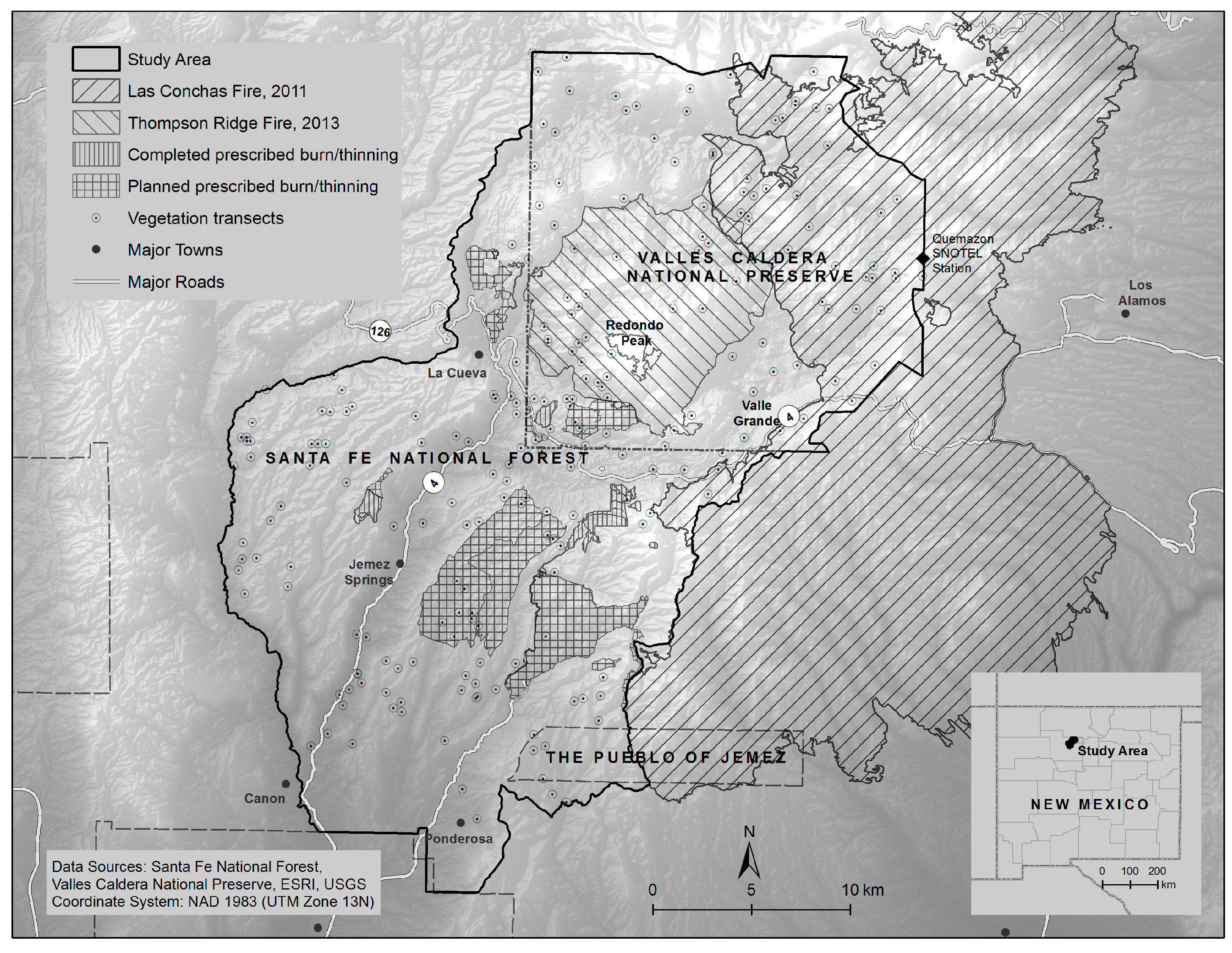
2.1. Study Area

The Collaborative Forest Landscape Restoration Project (CFLRP) area of the Southwest Jemez Mountains, in north-central New Mexico, USA, covers over 85,000 hectares, of which 52% is managed by the Santa Fe National Forest, 41% by the Valles Caldera National Preserve (National Park Service), 4% by private land owners, and 3% by the Pueblo of Jemez (Figure 1). Elevation ranges from about 1700 m to 3370 m (Redondo Peak), and the climate is generally semi-arid to continental [61]. Mean annual precipitation over the past 31 years (1981–2012), based on the nearest Snow Telemetry (SNOTEL) station (Quemazon station; located 13 km northeast of Redondo Peak), is 711 mm equally contributed by summer monsoon rainfall and wintertime snowfall [62].

The Valles Caldera National Preserve (VALL) and the adjoining Santa Fe National Forest (SFNF) are a complex region in terms of vegetation types and land cover dynamics. Forests (mixed conifer, ponderosa, and aspen), woodlands (piñon-juniper and oak), and grasslands (mostly alpine meadows) constitute the structural diversity of the landscape [63]. Ponderosa pine forests cover 34.37% of the study area, spruce-fir forests cover 29.53%, piñon-juniper woodlands cover 16.22%, grasslands cover 9.81%, oak woodlands cover 3.59%, sagebrush covers 3.30%, and aspen forests cover 3.16% of the total project area [64]. The dominant tree species are ponderosa pine (Pinus ponderosa Douglas ex Loudon), white fir (Abies concolor (Gordon & Glend.) Lindl. ex Hildebr.), blue spruce (Picea pungens Engelm.), Douglas fir (Pseudotsuga menziesii (Mirb.) Franco), piñon pine (Pinus edulis Engelm.), Rocky Mountain juniper (Juniperus scopulorum Sarg.), one-seed juniper (Juniperus monosperma Sarg.), alligator juniper (Juniperus deppeana Steud.), and quaking aspen (Populus tremuloides Michx.).

Recent large-scale fire events (especially the Las Conchas fire of 2011 and the Thompson Ridge fire of 2013) in the VALL and adjoining SFNF left very few to no trees across large areas, which have been recolonized mostly by shrubs and aspen saplings. Stand age, tree height, and tree density are the major attributes of the structural diversity of these complex forested ecosystems. Mature and old growth structures, open meadows, aspen stands, and understory diversity have decreased due to the increased forest density and recent wildfires [65]. To restore these altered forests, the CFLRP team, in conjunction with the managers at VALL and SFNF, have planned mechanical thinning and prescribed burning treatments for the study area. Some of the areas have already been treated with the aim of completion in coming years (Figure 1).

2.2. Field Data

A total of 224 permanent transects were established for annual vegetation monitoring in the study area. We used a systematic random sampling design to cover a range of vegetation types, canopy cover, and aspects while selecting these plots. There were 67 ponderosa transects, 59 spruce-fir transects, 36 piñon-juniper transects, 29 grassland transects, 17 oak transects, and 16 aspen transects. A 200 m transect was surveyed along a randomly selected bearing. If the transect appeared to cross a boundary between vegetation types, the bearing was chosen again and/or the transect length was reduced to 100 m. This helped to maintain a uniform vegetation type throughout the entire length of each transect. The transects were surveyed between May and August 2014. At every 40 m on the 200 m transect (or every 20 m on a 100 m transect), the density of live trees was estimated via the point-quarter method [66,67]. Tree density was calculated as:

$$\text{Absolute density }=\bar{\lambda }=\frac{{\left(4n\right)}^2}{{\left({{\displaystyle \sum }}_{i=1}^n{{\displaystyle \sum }}_{j=1}^4{R}_{ij}\right)}^2}$$

(1)

where n is the number of sampling points in a transect (=5); 4n is the total number of observations in the whole transect (=20); i is a sampling point in a transect (i = 1, …, n); j is a quarter at a transect point (j = 1, …, 4); and R_ij is the distance measured to the tree at the transect point i in quarter j [63].

2.3. Remote Sensing Data Acquisition and Processing

Standard Landsat 8 products provided by the United States Geological Survey (USGS) Earth Resources Observation and Science Center (EROS) were acquired for path 34 and row 35 (16 June 2014) with complete coverage of the study area. This level 1 product consisted of quantized and calibrated scaled Digital Numbers (DN) representing multispectral image data. The DN values were rescaled into radiance or the Top of Atmosphere (TOA) reflectance using the corresponding radiometric rescaling coefficients [68]. We used the equation for sun angle-corrected reflectance provided by the USGS [69]:

$${\rho }_{\lambda }=\frac{M_{\rho }{\mathrm{Q}}_{\mathrm{cal}}+{\mathrm{A}}_{\rho }}{\mathrm{Sin}({\theta }_{SE})}$$

(2)

where ${\rho }_{\lambda }$ is the TOA planetary reflectance; $M_{\rho }$ is the multiplicative rescaling factor; ${\mathrm{A}}_{\rho }$ is the additive rescaling factor; ${\mathrm{Q}}_{\mathrm{cal}}$ are the standard product pixel values or digital numbers (DN); and ${\theta }_{SE}$ is the local sun elevation angle. Bands 2 through 7 were used, as they have the same spatial resolution and have been used for vegetation analysis in the past [70,71]. The bands were: band 2 (blue: 450–510 nm), band 3 (green: 530–590 nm), band 4 (red: 640–670 nm), band 5 (near infrared: 0.85–0.88 µm), band 6 (short wave infrared: 1.57–1.65 µm), and band 7 (short wave infrared: 2.11–2.29 µm)) [69]. Rescaling into the TOA reflectance values was achieved by applying the equation above using Earth Resources Data Analysis System (ERDAS) Imagine^® software 2016. The TOA reflectance values for the sampling sites were extracted from the multispectral image by overlaying geographic coordinate points representing sampling locations in ERDAS Imagine^® software 2016. Due to the significant loss of information when resampled to six pixels (180 m × 180 m), the sampling locations represented 30 × 30 m pixels intersecting each field transect where similar continuous vegetation cover was evident.

2.4. Data Analysis

We used two-way analysis of variance (ANOVA) to analyze the overall variation in the field-based tree density means. Density was used as the dependent variable, and vegetation types (aspen, piñon-juniper, ponderosa, and spruce fir) and burn status (burned or not burned) due to the recent fire events of 2011 and 2013 were used as explanatory variables in a fully crossed model. There were 43 burned transects among the 178 transects under consideration for this analysis. A post-hoc Tukey test was also performed for the pairwise analysis of means when an overall difference was detected in density across vegetation types and burn status [72].

We used bands 2 to 7 and the Normalized Difference Vegetation Index (NDVI), the Difference Vegetation Index (DVI), the Simple Ratio (SR), and the Normalized Difference band 5 and band 7 (ND57) as predictor variables to model field tree density estimates in R statistical platform [24,30,73]). The formulas for each ratio are as follows: NDVI = (band 5 − band 4)/(band 5 + band 4); DVI = band 5 – band 4; SR1 = band 5/band 4; SR2 = band 6/band 4; SR3 = band 5/band 7; ND57 = (band 5 – band 7)/(band 5 + band 7) (modified from [4]). Log-transformed values of tree density were used as the independent variable to minimize the high range of density values.

As a first approach, linear regression was performed between measured density and bands or ratios (band 2, band 3, band 4, band 5, band 6, band 7, NDVI, DVI, ND57, SR1, SR2, and SR3) for all of the transects. We used forward stepwise selection to select the model for all of the transects at once. Subsequently, individual models were produced restricting values for each vegetation type: ponderosa pine, spruce-fir (mixed conifer), piñon-juniper, and aspen. We obtained vegetation classification data from the Santa Fe National Forest GIS data source [74]. Grasslands were excluded from the analysis as they have either zero or very few trees, and the areas dominated with sagebrush in the lower elevations were also exlcuded. Oak (mostly Gambel Oak: Quercus gambelii Nutt.; and Sonoran scrub oak: Quercus turbinella Greene) in the study area are considered shrubs; individual plants are typically not tall enough to reach top canopy heights and cover only 3.59% of the study area. Therefore, oak shrubland was also excluded from the analysis. After analyzing all individual bands, vegetation indices, and all possible combinations of the explanatory variables, the models with the greatest values of R² and adjusted R² values, and the lowest values of corrected Akaike Information Criteria (AICc) were selected [4,75]. The residual plots of each regression model did not show specific patterns, suggesting good fit for the models, and the normality plot of the residuals also supported proper fit. The pixel values resulting from the best respective models were used as an estimate of tree density for individual vegetation types.

The accuracy of the models was tested using a k-fold cross-validation approach, where the dataset is divided into roughly equal blocks and the model is constructed using all the blocks but one [76]. The model is then tested for the remaining block and the process is repeated k times resulting in an averaged estimated error [77]. We used 5-fold cross-validation (k = 5; [76]) because of the low number of observations for each vegetation type. Based on each of the five test cases’ residuals, an average mean square error value was produced for each of the models analyzed, which was used for the model’s predictive power. Individual regression models that were significant at the 95% confidence level were used to predict the density for each of the four vegetation types based on Landsat reflectance values and/or band ratios. As a logarithmic transformation was used to formulate the model, the values were transformed back to the actual density values in ERDAS Imagine^® to obtain the tree density map for each of the vegetation types. In ArcMap™, tree density was categorized into five classes for each of the vegetation types based on the management perspectives: zero density, low density (1–100 trees/ha), medium density (101–500 trees/ha), high density (501–1000 trees/ha), and very high density (>1000 trees/ha). Further, we combined the densities for different vegetation types using the raster mosaic tool in ArcMap™, and compared the areas covered by density classes in these areas: burned in 2011, burned in 2013, treated (mechanical thinning and prescribed fire) before June 2014, planned for immediate restoration treatment, and neither burned nor treated.

3. Results

3.1. Measured Tree Density

Based on the ground sampling data, tree density did not statistically differ by vegetation type. The trees were distributed at an average of 300 to 500 individuals/ha. In addition, unburned sites had significantly more trees (541 trees/ha) than the burned sites (107 trees/ha; main effect: F_{1, 171} = 2.933, p <0.001; Figure 2). Even though burned sites averaged more than 100 trees/ha, most of the transects had a very low number of live trees. Field observation showed that the high density of trees in the burned sites is due to the high regeneration of aspen.

3.2. Model Selection and Cross-Validation

Among all 12 explanatory variables, band ratios ND57, SR1, and DVI produced the best prediction for the combination of all vegetation types, as depicted by low values of AICc and the highest values of R² and adjusted R² (

Table 1. Corrected Akaike Information Criteria (AICc), R², adjusted R², and mean square error (MS) for the multiple regression models between density and combination of bands and vegetation indices for the entire area and for each vegetation type. Intercept and coefficients refer to the regression models used in the prediction. The values in bold show the best models selected.

Vegetation Types *	AICc	R2	Adj R2	MS **	Models ***
All	681.90	0.24	0.23	3.82	d^ = 4.03 + 5.89 ND57
(n = 178)	629.70	0.44	0.43	3.05	d^ = 7.96 + 17.72 ND57 − 2.50SR1
	623.80	0.46	0.45	3.04	d^ = 7.54 + 18.60 ND57 − 3.17 SR1 + 17.64 DVI
ASP	41.90	0.92	0.91	0.59	d^ = 3.50 + 19.94 ND57 − 2.26 SR3
(n = 16)	41.10	0.94	0.92	0.57	d^ = 1.19 + 24.76 ND57 − 2.70 SR3 + 26.86 band4
	33.40	0.97	0.96	0.36	d^ = 21.06 + 21.16 ND57 − 1.99 SR3 + 284.01 band4 − 478.56 band2
P-J	105.30	0.34	0.32	1.1	d^ = 8.63 − 22.73 band4
(n = 36)	96.80	0.52	0.49	0.86	d^ = 3.25 − 50.03 band4 + 84.74 band2
PON	207.00	0.35	0.32	1.26	d^ = 7.88 − 47.02 band7 + 66.15 band3 − 0.87 SR3
(n = 67)	200.00	0.43	0.40	1.15	d^ = 10.59 − 11.50 band7 + 9.50 band3 − 5.71 SR3 + 23.32 ND57
	199.00	0.46	0.42	1.10	d^ = 13.51 + 4.93 band7 − 24.93 band3 − 6.39 SR3 + 28.23 ND57 − 0.95 SR2
S-F	226.80	0.60	0.57	3.07	d^ = 3.87 + 2.14 ND57 − 6.12 SR1 + 38.20 NDVI − 1.78 SR2 + 2.57 SR3
(n = 59)	225.80	0.63	0.59	2.81	d^ = 2.85 − 1.32 ND57 − 7.87 SR1 + 41.36 NDVI − 1.82 SR2 + 4.24 SR3 + 21.87 DVI
	223.80	0.66	0.62	4.42	d^ = 6.67 − 11.46 ND57 − 8.68 SR1 + 37.32 NDVI − 1.81 SR2 + 5.58 SR3 + 55.51 DVI − 29.87 band7

* All, All points; ASP, Aspen, S-F, Spruce-Fir; PON, Ponderosa; P-J, Piñon-Juniper; NDVI, Normalized Difference Vegetation Index; DVI, Difference Vegetation Index; SR, Simple Ratio; and ND57, Normalized Difference band 5 and band 7. ** MS refers to the mean square error (trees/ha) reported from 5-fold cross validation of each model. *** log (density + 1) was used to deal with 0 density values, d^ refers to estimated density.

). For the best models, these values ranged from 33.40 to 223.80 (AICc), 0.46 to 0.97 (R²), and 0.42 to 0.96 (adjusted R²; Table 1). Non-transformed bands (band 4 and band 2) were sufficient to predict piñon-juniper density, but a combination of bands and band ratios produced the best models for aspen, ponderosa, and spruce-fir areas. Using a 5-fold cross validation approach, mean error estimates for the best models were 0.36 trees/ha for aspen (standard deviation (SD) = 0.19, n = 5), 0.86 trees/ha for pinyon-juniper (SD = 0.66, n = 5), 1.10 trees/ha for ponderosa pine (SD = 0.46, n = 5), and 4.42 trees/ha for spruce-fir (SD = 3.48, n = 5).

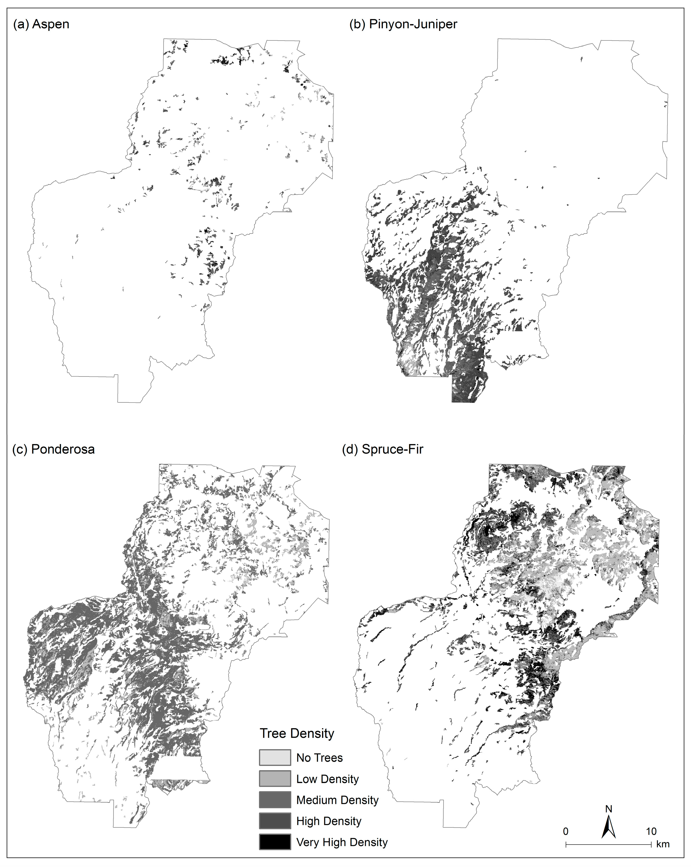
3.3. Tree Density Estimation

Based on the selected models, 4.21% of the areas classified as aspen and 7.69% of spruce-fir did not have trees, but most of the areas dominated by piñon-juniper and ponderosa had at least some trees (Figure 3). Most areas dominated by these four vegetation types (71.22% of aspen, 94.67% of piñon-juniper, 71.21% of ponderosa, and 55.30% of spruce-fir) had more than 100 trees per hectare, and more than 1000 trees per hectare were present in 13.14% of the spruce-fir areas (Figure 3 and Figure 4). A high proportion of piñon-juniper woodlands (54.11%) had more than 500 trees per hectare. Overall, 58.37% of the total study area had more than 100 trees per hectare, and 19% of the area had less than 100 trees per hectare.

4. Discussion

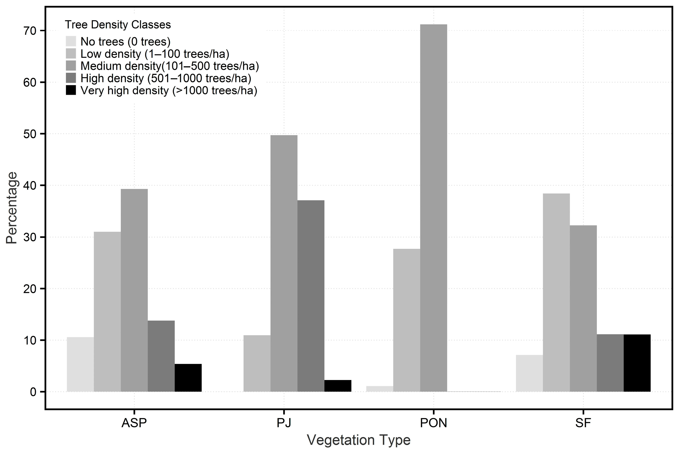
4.1. Current Forest Conditions

As of June 2014, most of the areas burned in the Las Conchas fire of 2011 had a low (62.90% of the burned area) or medium (23.69% of the burned area) density of live trees. We estimated similar composition in the areas burned in the Thompson Ridge fire of 2013 (

Table 2. Tree density as of June 2014.

Tree Density Class ↓	Area (%) *
Area (ha) →	Fire 2011 (9962.46)	Fire 2013 (8402.94)	Treated (670.23)	Planned (5793.48)	Not Treated (45361.71)
No trees	7.59	16.45	0.26	0.36	0.43
Low density (1–100 trees/ha)	62.90	44.54	45.29	18.35	16.08
Medium density (101–500 trees/ha)	23.69	32.40	42.22	64.08	56.82
High density (501–1000 tress/ha)	3.14	4.02	5.48	14.45	19.86
Very high density (>1000 trees/ha)	2.68	2.59	6.75	2.77	6.81

* Top values are in bold face.

). In addition, the areas treated with prescribed fire and thinning demonstrated similar patterns, with more than 87% of the treated areas estimated to have a low and medium density of trees. On the other hand, more than 80% of the area planned for immediate restoration treatments consisted of greater than 100 trees per hectare. Similarly, the remainder of the area which was neither treated nor planned for immediate treatment were also dominated by a medium to very high density of trees (83.49% of the area).

We predicted that conifer-dominated forests in the Jemez Mountains have a high density of trees, and that Landsat 8 imagery, particularly a combination of individual bands (bands 2, 3, 4, and 7) and transformed bands (ND57, NDVI, and simple ratios) can be a useful method for monitoring tree density in this region, which has complex vegetation types and topography. The high density of trees predicted by our model corresponds with [78], who also reported very high ponderosa pine densities in the Monument Canyon area of the Jemez Mountains. The density of young trees has been increasing in these forests due to the absence of fire and changes in management practices such as grazing [78,79].

The forests of the study area have significantly departed from historic conditions, with a higher tree density leading to a higher risk of losing key ecosystem components due to a high fire risk [65]. In similar mixed-conifer forests in Arizona, historical tree densities were estimated at ~140 live trees/ha [80]. Our density estimates for the Jemez Mountains study area greatly exceed this, with more than 500 live trees/ha in more than 36% of the area. These high densities are primarily in areas which were not burned in the big fires of 2011 and 2013, and have not yet been treated with thinning or prescribed burning, but are considered for either immediate or future restoration treatments. The method we use here could therefore help managers to identify and prioritize areas with higher tree densities to consider for upcoming restoration treatments. Our estimation of the current conditions of these forests also demonstrates the effectiveness of treatment procedures, as indicated by the lower tree densities in the treated areas.

4.2. Predicting Tree Density

Model performance, a derivative of reflectance, is influenced by the leaf area index (LAI), and several factors such as leaf structure, leaf orientation, and ground exposure have an impact on LAI [81]. Model performance for the aspen-dominated areas was better than for the other vegetation types because of the broad leaf type which allows less ground exposure, thereby reducing background noise. Among the conifer-dominated forests, the model for spruce-fir performed better, because of the higher density branches and needles reducing background influence, than the ponderosa pine- and pinyon-juniper-dominated areas. In addition to the plant architecture, the optical properties of the atmosphere have an impact on the TOA reflectance of the shortwave bands [82], which could have resulted in the low accuracy pinyon-juniper and ponderosa pine models. Even though the inclusion of band 2 produced a better ponderosa pine model, we excluded it from the process to avoid overprediction because of its high correlation with band 3 (r = 0.98).

The near and middle infrared bands, individually or used in ratios, had an important role in the predictive capabilities of our models. Similar studies have reported that infrared bands are effective for forest density prediction, including [23], who postulated that dense stands have higher infrared reflectance than low density stands. However, the conifer forests in our study did not show strong correlation between infrared bands and tree density because of the leaf orientation and leaf structure [83]. Studies have shown that the amount of near infrared energy reflected in this region of the spectrum is controlled by the spongy mesophyll layers in green leaves due to internal scattering at the cell wall–air interfaces within the leaf [83]. Therefore, the amount of green healthy leaves present in a specific area will have an impact on the overall near infrared reflectance. Similarly, there is a strong relationship between reflectance in the middle infrared region from 1.3 to 2.5 µm and the amount of water present in the leaves of a plant canopy, which is stored in the spongy mesophyll layers of the leaves. Water is a good absorber of middle infrared energy, so the greater the turgidity of the leaves, the lower the middle infrared reflectance [83]. Because of this, the high predictability of vegetation density by ratios using bands 5 and 7 (near infrared and middle infrared) in combination with bands 4 and 2 (visible bands controlled by photosynthetic pigments) was expected.

Nonetheless, the strength of the relationship between the visible and infrared bands with tree density is ecosystem dependent [83]. We found that some bands and band ratios explained more of the tree density in broadleaf aspen forests, followed by the spruce-fir, piñon-juniper, and ponderosa pine forests, respectively. Using ratios as explanatory variables in this study, the R² values for the predicted live tree density in different types of coniferous forests achieved values between 0.46 and 0.66, which are higher than those found for the lodgepole pine forest (R² = 0.34) in Yellowstone National Park [20]. The results from this study are comparable to predictions in commercially managed and mixed-aged loblolly pine forests in Texas (R² = 0.60; [23]). The R² values for aspen forests in this study were higher than those in similar studies of homogenous and broad-leaved forested landscapes in Iran studied by [4] as well. We also found similar results for spruce-fir mixed forests (R² = 0.63) compared to those that were reported for mixed forests in Turkey [22].

In our study, even though the Landsat data had been geometrically corrected prior to analysis, some areas showed an unusually predicted high density of pinyon-juniper trees, particularly in steep slopes (Figure 3 and Figure 4b). This is probably related to a strong viewing angle effect causing lower reflectance values for the visible wavelengths in such areas [84]. Other possible sources of error could be related to the transect method of sampling trees rather than squared plots, as the density was predicted for pixels of 30 × 30 square meters rather than for a line that potentially crossed multiple pixels.

5. Conclusions

The use of Landsat 8 imagery to predict tree density patterns in areas with complex vegetation types, terrain, and wildfire history is an important advance that will aid in management decisions. Forests in Southwestern USA are increasingly the targets of study and for the implementation of restoration treatments (e.g., [48,85,86,87]), and models based on remotely sensed spectral reflectance values provide a landscape-scale perspective for areas to be treated by mechanical thinning, prescribed fire, or other treatments based on spatial patterns of tree density for each vegetation type. Forest managers could use a combination of on-the-ground density data, calculated from measurements such as the point-center-quarter method [88], and combine these with vegetation indices to predict tree density. The use of near infrared and middle infrared spectral bands should be considered for predicting tree density, either as individual predictors or in band ratios, as these provide the most accurate results. However, the estimation could be influenced by plant architecture, such as leaf structure, leaf orientation, and ground exposure. These results could be further improved by measuring tree data via a sampling design fitted to match the spatial resolution of satellite imagery and an integrated analysis with data from active remote sensing techniques. Further steps in remote sensing research in this region should include the estimation of other forest parameters, such as DBH, aboveground biomass, and stand age characteristics using remote sensing data. Forest managers could use our findings to identify the most susceptible areas for uncontrolled wildfire, and to consider those areas for immediate restoration plans.

References

1. Roberts, M.R.; Gilliam, F.S. Patterns and mechanisms of plant diversity in forested ecosystems: Implications for forest management. Ecol. Appl. 1995, 5, 969–977. [Google Scholar] [CrossRef]
2. Franklin, J.F.; Spies, T.A.; Van Pelt, R.; Carey, A.B.; Thornburgh, D.A.; Berg, D.R.; Lindenmayer, D.B.; Harmon, M.E.; Keeton, W.S.; Shaw, D.C.; et al. Disturbances and structural development of natural forest ecosystems with silvicultural implications, using Douglas-fir forests as an example. For. Ecol. Manag. 2002, 155, 399–423. [Google Scholar] [CrossRef]
3. Propastin, P. Relations between Landsat ETM+ imagery and forest structure parameters in tropical rainforests: A case study from Lore-Lindu National Park in Sulawesi, Indonesia. EARSeL eProc. 2009, 8, 93–106. [Google Scholar]
4. Mohammadi, J.; Joibary, S.S.; Yaghmaee, F.; Mahiny, A.S. Modelling forest stand volume and tree density using Landsat ETM+ data. Int. J. Remote Sens. 2010, 31, 2959–2975. [Google Scholar] [CrossRef]
5. Rocchini, D. Seeing the unseen by remote sensing: Satellite imagery applied to species distribution modelling. J. Veg. Sci. 2013, 24, 209–210. [Google Scholar] [CrossRef]
6. Varga, P.; Chen, H.Y.; Klinka, K. Tree-Size diversity between single-and mixed-species stands in three forest types in western Canada. Can. J. For. Res. 2005, 35, 593–601. [Google Scholar] [CrossRef]
7. McRoberts, R.E.; Winter, S.; Chirici, G.; Hauk, E.; Pelz, D.R.; Moser, W.K.; Hatfield, M.A. Large-Scale spatial patterns of forest structural diversity. Can. J. For. Res. 2008, 38, 429–438. [Google Scholar] [CrossRef]
8. Legendre, P.; Dale, M.R.; Fortin, M.J.; Gurevitch, J.; Hohn, M.; Myers, D. The consequences of spatial structure for the design and analysis of ecological field surveys. Ecography 2002, 25, 601–615. [Google Scholar] [CrossRef]
9. Edwards, T.C.; Cutler, D.R.; Zimmermann, N.E.; Geiser, L.; Moisen, G.G. Effects of sample survey design on the accuracy of classification tree models in species distribution models. Ecol. Model. 2006, 199, 132–141. [Google Scholar] [CrossRef]
10. Heywood, V. Global Biodiversity Assessment; Cambridge University Press: Cambridge, UK, 1995; ISBN 9780521564816. [Google Scholar]
11. Palmer, M.W. Species–Area curves and the geometry of nature. In Scaling Biodiversity, 1st ed.; Storch, D., Marquet, P.L., Brown, J.H., Eds.; Cambridge University Press: Cambridge, UK, 2007; pp. 15–31. ISBN 9780521876025. [Google Scholar]
12. Ozdemir, I.; Karnieli, A. Predicting forest structural parameters using the image texture derived from WorldView-2 multispectral imagery in a dryland forest, Israel. Int. J. Appl. Earth Obs. Geoinform. 2011, 13, 701–710. [Google Scholar] [CrossRef]
13. Hernández-Stefanoni, J.L.; Gallardo-Cruz, J.A.; Meave, J.A.; Rocchini, D.; Bello-Pineda, J.; López-Martínez, J.O. Modeling α-and β-diversity in a tropical forest from remotely sensed and spatial data. Int. J. Appl. Earth Obs. Geoinform. 2012, 19, 359–368. [Google Scholar] [CrossRef]
14. Kerr, J.T.; Ostrovsky, M. From space to species: Ecological applications for remote sensing. Trends Ecol. Evol. 2003, 18, 299–305. [Google Scholar] [CrossRef]
15. Hudak, A.T.; Crookston, N.L.; Evans, J.S.; Falkowski, M.J.; Smith, A.M.; Gessler, P.E.; Morgan, P. Regression modeling and mapping of coniferous forest basal area and tree density from discrete-return lidar and multispectral satellite data. Can. J. Remote Sens. 2006, 32, 126–138. [Google Scholar] [CrossRef]
16. Nagendra, H. Using remote sensing to assess biodiversity. Int. J. Remote Sens. 2001, 22, 2377–2400. [Google Scholar] [CrossRef]
17. Palmer, M.W.; Earls, P.; Hoagland, B.W.; White, P.S.; Wohlgemuth, T. Quantitative tools for perfecting species lists. Environmetrics 2002, 13, 121–137. [Google Scholar] [CrossRef]
18. Hernández-Stefanoni, J.; Dupuy, J. Mapping species density of trees, shrubs and vines in a tropical forest, using field measurements, satellite multispectral imagery and spatial interpolation. Biodivers. Conserv. 2007, 16, 3817–3833. [Google Scholar] [CrossRef]
19. Feilhauer, H.; Schmidtlein, S. Mapping continuous fields of forest α- and β-diversity. Appl. Veg. Sci. 2009, 12, 429–439. [Google Scholar] [CrossRef]
20. Jakubauskas, M.E.; Price, K.P. Empirical relationships between structural and spectral factors of Yellowstone lodgepole pine forests. Photogramm. Eng. Remote Sens. 1997, 63, 1375–1380. [Google Scholar]
21. Smith, A.M.; Falkowski, M.J.; Hudak, A.T.; Evans, J.S.; Robinson, A.P.; Steele, C.M. A cross-comparison of field, spectral, and lidar estimates of forest canopy cover. Can. J. Remote Sens. 2009, 35, 447–459. [Google Scholar] [CrossRef]
22. Kahriman, A.; Günlü, A.; Karahalil, U. Estimation of crown closure and tree density using Landsat TM satellite images in mixed forest stands. J. Indian Soc. Remote Sens. 2014, 42, 559–567. [Google Scholar] [CrossRef]
23. Sivanpillai, R.; Smith, C.T.; Srinivasan, R.; Messina, M.G.; Wu, X.B. Estimation of managed loblolly pine stand age and density with Landsat ETM+ data. For. Ecol. Manag. 2006, 223, 247–254. [Google Scholar] [CrossRef]
24. Tucker, C.J.; Fung, Y.; Keeling, C.D.; Gammon, R.H. Relationship between atmospheric CO2 variations and a satellite-derived vegetation index. Nature 1986, 319, 195–199. [Google Scholar] [CrossRef]
25. Song, C.; Zhang, Y. Forest Cover in China from 1949 to 2006. In Reforesting Landscapes: Linking Pattern and Process, Landscape Series; Nagendra, H., Southworth, J., Eds.; Springer: Dordrecht, The Netherlands, 2010; Volume 10, pp. 341–356. ISBN 978-1-4020-9656-3. [Google Scholar]
26. Gould, W. Remote sensing of vegetation, plant species richness, and regional biodiversity hotspots. Ecol. Appl. 2000, 10, 1861–1870. [Google Scholar] [CrossRef]
27. Fairbanks, D.H.; McGwire, K.C. Patterns of floristic richness in vegetation communities of California: Regional scale analysis with multi-temporal NDVI. Glob. Ecol. Biogeogr. 2004, 13, 221–235. [Google Scholar] [CrossRef]
28. Gillespie, T.W. Predicting woody-plant species richness in tropical dry forests: A case study from south Florida, USA. Ecol. Appl. 2005, 15, 27–37. [Google Scholar] [CrossRef]
29. Rocchini, D.; Hernández-Stefanoni, J.L.; He, K.S. Advancing species diversity estimate by remotely sensed proxies: A conceptual review. Ecol. Inform. 2015, 25, 22–28. [Google Scholar] [CrossRef]
30. Lu, D.; Mausel, P.; Brondızio, E.; Moran, E. Relationships between forests stand parameters and Landsat TM spectral responses in the Brazilian Amazon Basin. For. Ecol. Manag. 2004, 198, 149–167. [Google Scholar] [CrossRef]
31. He, K.S.; Zhang, J.; Zhang, Q. Linking variability in species composition and MODIS NDVI based on beta diversity measurements. Acta Oecol. 2009, 35, 14–21. [Google Scholar] [CrossRef]
32. Meng, R.; Dennison, P.E.; Huang, C.; Moritz, M.A.; D’Antonio, C. Effects of fire severity and post-fire climate on short-term vegetation recovery of mixed-conifer and red fir forests in the Sierra Nevada Mountains of California. Remote Sens. Environ. 2015, 171, 311–325. [Google Scholar] [CrossRef]
33. Feilhauer, H.; He, K.S.; Rocchini, D. Modelling species distribution using niche-based proxies derived from composite bioclimatic variables and MODIS NDVI. Remote Sens. 2012, 4, 2057–2075. [Google Scholar] [CrossRef]
34. Vacchiano, G.; Motta, R. An improved species distribution model for Scots pine and downy oak under future climate change in the NW Italian Alps. Ann. For. Sci. 2015, 72, 321–334. [Google Scholar] [CrossRef]
35. Irisarri, J.G.N.; Oesterheld, M.; Paruelo, J.M.; Texeira, M.A. Patterns and controls of above-ground net primary production in meadows of Patagonia: A remote sensing approach. J. Veg. Sci. 2012, 23, 114–126. [Google Scholar] [CrossRef]
36. Borowik, T.; Pettorelli, N.; Sönnichsen, L.; Jędrzejewska, B. Normalized difference vegetation index (NDVI) as a predictor of forage availability for ungulates in forest and field habitats. Eur. J. Wildl. Res. 2013, 59, 675–682. [Google Scholar] [CrossRef]
37. Vogelmann, J.E.; Tolk, B.; Zhu, Z. Monitoring forest changes in the southwestern United States using multitemporal Landsat data. Remote Sens. Environ. 2009, 113, 1739–1748. [Google Scholar] [CrossRef]
38. Madurapperuma, B.D.; Kuruppuarachchi, K.A.J.M. Detecting land-cover change using mappable vegetation related indices: A case study from Sinharaja Man and the Biosphere Reserve. J. Trop. For. Environ. 2014, 4, 50–58. [Google Scholar]
39. Franklin, S.E.; Hall, R.J.; Smith, L.; Gerylo, G.R. Discrimination of conifer height, age and crown closure classes using Landsat-5 TM imagery in the Canadian Northwest Territories. Int. J. Remote Sens. 2003, 24, 1823–1834. [Google Scholar] [CrossRef]
40. Freitas, S.R.; Mello, M.C.; Cruz, C.B. Relationships between forest structure and vegetation indices in Atlantic Rainforest. For. Ecol. Manag. 2005, 218, 353–362. [Google Scholar] [CrossRef]
41. Fulé, P.Z.; Covington, W.W.; Moore, M.M. Determining reference conditions for ecosystem management of southwestern ponderosa pine forests. Ecol. Appl. 1997, 7, 895–908. [Google Scholar] [CrossRef]
42. Moore, M.M.; Huffman, D.W.; Fulé, P.Z.; Covington, W.W.; Crouse, J.E. Comparison of historical and contemporary forest structure and composition on permanent plots in southwestern ponderosa pine forests. For. Sci. 2004, 50, 162–176. [Google Scholar]
43. Covington, W.W.; Moore, M.M. Postsettlement changes in natural fire regimes and forest structure. J. Sustain. For. 1994, 2, 153–181. [Google Scholar] [CrossRef]
44. Kenneth, L.; Dye, I.I.; Ueckert, D.N.; Whisenant, S.G. Redberry juniper-herbaceous understory interactions. J. Range Manag. 1995, 48, 100–107. [Google Scholar] [CrossRef]
45. Touchan, R.; Allen, C.D.; Swetnam, T.W. Fire history and climatic patterns in ponderosa pine and mixed-conifer forests of the Jemez Mountains, northern New Mexico. In Fire Effects in Southwestern Forests, Proceedings of the Second La Mesa Fire Symposium RM-GTR-286, Los Alamos, New Mexico, USA, 29–31 March 1996; USDA-Rocky Mountain Forest and Range Experiment Station: Fort Collins, CO, USA, 1996; pp. 33–46. [Google Scholar]
46. Miller, C.; Urban, D.L. Modeling the effects of fire management alternatives on Sierra Nevada mixed-conifer forests. Ecol. Appl. 2000, 10, 85–94. [Google Scholar] [CrossRef]
47. Lydersen, J.M.; Collins, B.M.; Miller, J.D.; Fry, D.L.; Stephens, S.L. Relating fire-caused change in forest structure to remotely sensed estimates of fire severity. Fire Ecol. 2016, 12, 99–116. [Google Scholar] [CrossRef]
48. Mast, J.N.; Fulé, P.J.; Moore, M.M.; Covington, W.W.; Waltz, A.E.M. Restoration of presettlement age structure of an Arizona ponderosa pine forest. Ecol. Appl. 1999, 9, 228–239. [Google Scholar] [CrossRef]
49. Kaye, J.P.; Hart, S.C.; Fulé, P.Z.; Covington, W.W.; Moore, M.M.; Kaye, M.W. Initial carbon, nitrogen, and phosphorus fluxes following ponderosa pine restoration treatments. Ecol. Appl. 2005, 15, 1581–1593. [Google Scholar] [CrossRef]
50. Finkral, A.J.; Evans, A.M. The effects of a thinning treatment on carbon stocks in a northern Arizona ponderosa pine forest. For. Ecol. Manag. 2008, 255, 2743–2750. [Google Scholar] [CrossRef]
51. Fulé, P.Z.; Crouse, J.E.; Cocke, A.E.; Moore, M.M.; Covington, W.W. Changes in canopy fuels and potential fire behavior 1880–2040: Grand Canyon, Arizona. Ecol. Model. 2004, 175, 231–248. [Google Scholar] [CrossRef]
52. Gass, T.M.; Robinson, A.P. A hierarchical analysis of stand structure, composition, and burn patterns as indicators of stand age in an Engelmann spruce–subalpine fir forest. Can. J. For. Res. 2007, 37, 884–894. [Google Scholar] [CrossRef]
53. Hayes, J.J.; Robeson, S.M. Spatial variability of landscape pattern change following a ponderosa pine wildfire in northeastern New Mexico, USA. Phys. Geogr. 2009, 30, 410–429. [Google Scholar] [CrossRef]
54. Lydersen, J.M.; North, M.P.; Collins, B.M. Severity of an uncharacteristically large wildfire, the Rim Fire, in forests with relatively restored frequent fire regimes. For. Ecol. Manag. 2014, 328, 326–334. [Google Scholar] [CrossRef]
55. Stevens, J.T.; Safford, H.D.; North, M.P.; Fried, J.S.; Gray, A.N.; Brown, P.M.; Dolanc, C.R.; Dobrowski, S.Z.; Falk, D.A.; Farris, C.A.; et al. Average stand age from forest inventory plots does not describe historical fire regimes in ponderosa pine and mixed-conifer forests of western North America. PLoS ONE 2016, 11, e0147688. [Google Scholar] [CrossRef] [PubMed]
56. Butera, M.K. A correlation and regression analysis of percent canopy closure versus TMS spectral response for selected forest sites in the San Juan National Forest, Colorado. IEEE Trans. Geosci. Remote Sens. 1986, 1, 122–129. [Google Scholar] [CrossRef]
57. Cohen, W.B.; Spies, T.A. Estimating structural attributes of Douglas Fir-western hemlock forest stands from Landsat and SPOT imagery. Remote Sens. Environ. 1992, 41, 1–17. [Google Scholar] [CrossRef]
58. Fiorella, M.; Ripple, W.J. Analysis of conifer forest regeneration using Landsat Thematic Mapper data. Photogramm. Eng. Remote Sens. 1993, 59, 1383–1388. [Google Scholar]
59. Peterson, D.L.; Westman, W.E.; Stephenson, N.J.; Ambrosia, V.G.; Brass, J.A.; Spanner, M.A. Analysis of forest structure using Thematic Mapper Simulator data. IEEE Trans. Geosci. Remote Sens. 1986, 24, 113–121. [Google Scholar] [CrossRef]
60. Oladi, J. Developing diameter at breast height (DBH) and a height estimation model from remotely sensed data. J. Agric. Sci. 2005, 7, 95–102. [Google Scholar]
61. Coop, J.D.; Givnish, T.J. Spatial and temporal patterns of recent forest encroachment in montane grasslands of the Valles Caldera, New Mexico, USA. J. Biogeogr. 2007, 34, 914–927. [Google Scholar] [CrossRef]
62. Zapata-Rios, X.; McIntosh, J.; Rademacher, L.; Troch, P.A.; Brooks, P.D.; Rasmussen, C.; Chorover, J. Climatic and landscape controls on water transit times and silicate mineral weathering in the critical zone. Water Resour. Res. 2015, 51, 6036–6051. [Google Scholar] [CrossRef]
63. Dick-Peddie, W.A.; Moir, W.H.; Spellenberg, R. New Mexico Vegetation: Past, Present, and Future; University of New Mexico Press: Albuquerque, NM, USA, 1999; ISBN 978-0-8263-2164-0. [Google Scholar]
64. SWJ-CFLRP. Southwest Jemez Mountains Collaborative Forest Landscape Restoration Proposal for Funding; Santa Fe National Forest and Valles Caldera National Preserve: Jemez Springs, NM, USA, 2010. [Google Scholar]
65. Reynolds, R.T.; Sanchez Meador, A.J.; Youtz, J.A.; Nicolet, T.; Mantonis, M.S.; Jackson, P.L.; DeLorenzo, D.G.; Graves, A.D. Restoring Composition and Structure in Southwestern Frequent-Fire Forests: A Science-Based Framework for Improving Ecosystem Resiliency; Gen. Tech. Rep. RMRSGTR-310; U.S. Department of Agriculture, Forest Service, Rocky Mountain Research Station: Fort Collins, CO, USA, 2013; 76 p. [Google Scholar]
66. Mitchell, K. Quantitative Analysis by the Point-Centered Quarter Method. Hobart and William Smith Colleges: Geneva, NY, USA. arXiv. 2015. Available online: https://arxiv.org/abs/1010.3303 (accessed on 25 August 2015).
67. Bryant, D.M.; Ducey, M.J.; Innes, J.C.; Lee, T.D.; Eckert, R.T.; Zarin, D.L. Forest community analysis and the point-centered quarter method. Plant Ecol. 2005, 175, 193–203. [Google Scholar] [CrossRef]
68. Bhardwaj, A.; Joshi, P.K.; Sam, L.; Singh, M.K.; Singh, S.; Kumar, R. Applicability of Landsat 8 data for characterizing glacier facies and supraglacial debris. Int. J. Appl. Earth Obs. Geoinf. 2015, 38, 51–56. [Google Scholar] [CrossRef]
69. USGS. Landsat 8 (L8) Data Users Handbook, version 1.0 (LSDS-1574); United States Geological Survey, Earth Resources Observation System (EROS): Sioux Falls, SD, USA, 2015. [Google Scholar]
70. Ding, Y.; Zhao, K.; Zheng, X.; Jiang, T. Temporal dynamics of spatial heterogeneity over cropland quantified by time-series NDVI, near infrared and red reflectance of Landsat 8 OLI imagery. Int. J. Appl. Earth Obs. Geoinf. 2014, 30, 139–145. [Google Scholar] [CrossRef]
71. Dube, T.; Mutanga, O. Evaluating the utility of the medium-spatial resolution Landsat 8 multispectral sensor in quantifying aboveground biomass in uMgeni catchment, South Africa. ISPRS J. Photogramm. Remote Sens. 2015, 101, 36–46. [Google Scholar] [CrossRef]
72. Scheiner, S.; Gurevitch, J. Design and Analysis of Ecological Experiments; Chapman and Hall: New York, NY, USA, 1998; ISBN 10:0412035618. [Google Scholar]
73. Venables, W.N.; Smith, D.M. An introduction to R; Network Theory Limited: East Sussex, UK, 2009; ISBN 0954612086. [Google Scholar]
74. United States Department of Agriculture Forest Service, Santa Fe National Forest GIS Data. Available online: https://www.fs.usda.gov/detail/r3/landmanagement/gis/?cid=stelprdb5203736 (accessed on 10 September 2015).
75. Stauffer, H.B. Contemporary Bayesian and Frequentist Statistical Research Methods for Natural Resource Scientists; John Wiley & Sons: Hoboken, NJ, USA, 2007; ISBN 978-0-470-16504-1. [Google Scholar]
76. Dobrowski, S.Z.; Safford, H.D.; Cheng, Y.B.; Ustin, S.L. Mapping mountain vegetation using species distribution modeling, image-based texture analysis, and object-based classification. Appl. Veg. Sci. 2008, 11, 499–508. [Google Scholar] [CrossRef]
77. Yang, L.; Huang, C.; Homer, C.G.; Wylie, B.K.; Coan, M.J. An approach for mapping large-area impervious surfaces: Synergistic use of Landsat-7 ETM+ and high spatial resolution imagery. Can. J. For. Res. 2003, 29, 230–240. [Google Scholar] [CrossRef]
78. Allen, C.D. A ponderosa pine natural area reveals its secrets. In Status and Trends of the Nation’s Biological Resources; Opler, P.A., Haecker, C.E., Eds.; US Geological Survey: Reston, VA, USA, 1998; Volume 2, pp. 551–552. [Google Scholar]
79. Sisk, T.D.; Prather, J.W.; Hampton, H.M.; Aumack, E.N.; Xu, Y.; Dickson, B.G. Participatory landscape analysis to guide restoration of ponderosa pine ecosystems in the American Southwest. Landsc. Urban Plan. 2006, 78, 300–310. [Google Scholar] [CrossRef]
80. Rodman, K.C.; Sánchez Meador, A.J.; Huffman, D.W.; Waring, K.M. Reference conditions and historical fine-scale spatial dynamics in a dry mixed-conifer forest, Arizona, USA. For. Sci. 2016, 62, 268–280. [Google Scholar] [CrossRef]
81. Darvishzadeh, R.; Skidmore, A.; Atzberger, C.; van Wieren, S. Estimation of vegetation LAI from hyperspectral reflectance data: Effects of soil type and plant architecture. Int. J. Appl. Earth Obs. Geoinform. 2008, 10, 358–373. [Google Scholar] [CrossRef]
82. Verhoef, W.; Bach, H. Coupled soil–leaf-canopy and atmosphere radiative transfer modeling to simulate hyperspectral multi-angular surface reflectance and TOA radiance data. Remote Sens. Environ. 2007, 109, 166–182. [Google Scholar] [CrossRef]
83. Jensen, J.R. Remote Sensing of Environment: An Earth Resource Perspective; Pearson Prentice Hall: Upper Saddle River, NJ, USA, 2007; ISBN 0131889508. [Google Scholar]
84. Song, C.; Woodcock, C.E. Monitoring forest succession with multitemporal Landsat images: Factors of uncertainty. IEEE Trans. Geosci. Remote Sens. 2003, 41, 2557–2567. [Google Scholar] [CrossRef]
85. North, M.; Innes, J.; Zald, H. Comparison of thinning and prescribed fire restoration treatments to Sierran mixed-conifer historic conditions. Can. J. For. Res. 2007, 37, 331–342. [Google Scholar] [CrossRef]
86. Korb, J.E.; Fulé, P.Z.; Stoddard, M.T. Forest restoration in a surface fire-dependent ecosystem: An example from a mixed conifer forest, southwestern Colorado, USA. For. Ecol. Manag. 2012, 269, 10–18. [Google Scholar] [CrossRef]
87. Erickson, C.C.; Waring, K.M. Old Pinus ponderosa growth responses to restoration treatments, climate and drought in a southwestern US landscape. Appl. Veg. Sci. 2014, 17, 97–108. [Google Scholar] [CrossRef]
88. Cottam, G.; Curtis, J.T. The use of distance measures in phytosociological sampling. Ecology 1956, 37, 451–460. [Google Scholar] [CrossRef]
Figure 1. Study area of the Southwest Jemez Mountains (Sandoval Co., NM, USA) showing major wildfires, treated areas as of 2014, planned areas for treatment, and distribution of sampling transects.
Forests 08 00287 g001
Figure 2. Measured density (individuals/ha) in forest stands burned in 2011 and 2013 vs. unburned stands in the Southwest Jemez Mountains, New Mexico, USA. Tuckey Honest Significant Difference (HSD) showed significant difference in the mean densities. Wider shaded areas represent a higher number of points. SD, standard deviation.
Forests 08 00287 g002
Figure 3. Percent of predicted density classes by vegetation type (ASP, Aspen; PJ, Piñon-Juniper; PON, Ponderosa; and SF, Spruce-Fir) in the Southwest Jemez Mountains, New Mexico, USA.
Forests 08 00287 g003
Figure 4. Predicted tree density maps by vegetation types: (a) Aspen, (b) Piñon-Juniper, (c) Ponderosa, and (d) Spruce Fir. (No trees: 0 trees, Low density: 1–100 trees/hectare, Medium density: 101–500 trees/hectare, High Density: 501–1000 trees/hectare, and Very high density: more than 1000 trees/hectare) in the Southwest Jemez Mountains, Sandoval Co., NM, USA.
Forests 08 00287 g004