Edyn: Dynamic Signaling of Changes to Forests Using Exponentially Weighted Moving Average Charts


1
Department of Forest Resources and Environmental Conservation, Virginia Polytechnic Institute and State University, 310 West Campus Drive, Blacksburg, VA 24061, USA
2
Department of Forest Ecosystems and Society, Oregon State University, Corvallis, OR 97331, USA
*
Author to whom correspondence should be addressed.
Forests 2017, 8(9), 304; https://doi.org/10.3390/f8090304
Submission received: 21 July 2017
/
Revised: 15 August 2017
/
Accepted: 18 August 2017
/
Published: 24 August 2017
(This article belongs to the Special Issue Remote Sensing of Forest Disturbance)
Abstract
:Remote detection of forest disturbance remains a key area of interest for scientists and land managers. Subtle disturbances such as drought, disease, insect activity, and thinning harvests have a significant impact on carbon budgeting and forest productivity, but current change detection algorithms struggle to accurately identify them, especially over decadal timeframes. We introduce an algorithm called Edyn, which inputs a time series of residuals from harmonic regression into a control chart to signal low-magnitude, consistent deviations from the curve as disturbances. After signaling, Edyn retrains a new baseline curve. We compared Edyn with its parent algorithm (EWMACD—Exponentially Weighted Moving Average Change Detection) on over 3500 visually interpreted Landsat pixels from across the contiguous USA, with reference data for timing and type of disturbance. For disturbed forested pixels, Edyn had a mean per-pixel commission error of 31.1% and omission error of 70.0%, while commission and omission errors for EWMACD were 39.9% and 65.2%, respectively. Edyn had significantly less overall error than EWMACD (F1 = 0.19 versus F1 = 0.13). These patterns generally held for all of the reference data, including a direct comparison to other contemporary change detection algorithms, wherein Edyn and EWMACD were found to have lower omission error rates for a category of subtle changes over long periods.
Keywords:
change detection; EWMACD; forest disturbance; Fourier; Landsat; quality control; remote sensing1. Introduction
Remote sensing, with Landsat in particular, has long been used to detect forest disturbance at a wide variety of scales [1,2,3,4]. Since the Landsat archive was made freely available, numerous change detection algorithms have been developed which use up to decades-long time series of observations to signal, quantify, and attribute forest disturbance [5,6,7,8,9,10,11]. These time series algorithms improve on more traditional bi-temporal, or image-to-image, approaches.
Disturbances that occur abruptly in the temporal domain such as clearcut harvests, fires and land-use conversions tend to be easier to detect than more subtle changes brought on by thinning, drought, insects and other within-class changes [12,13,14,15]. These subtle changes are harder to detect but may still contribute significantly to the overall forest carbon budget [16,17,18]. For example, Cohen et al. [13] found evidence of a more general forest decline, defined there as canopy loss not associated with or attributable to other common classes (in the case of that study: fire, harvest, wind, water, land use conversion, or debris), that has a wide extent and an increasingly sizable impact on forest productivity and carbon flow. Given that these subtle changes can affect the structure and functioning of forests over large areas, there is a great need to identify them and other such within-class changes (e.g., a thinned or drought-stressed forest) using remote sensing.
Exponentially Weighted Moving Average Change Detection (EWMACD) [5] is a freely available, open-source [19] pixel-level time series change detection algorithm originally designed to detect a wide variety of persistent changes to forested pixels. EWMACD uses exponentially weighted moving average (EWMA) control charts to analyze residual values resulting from fitting the input time series to harmonic (e.g., Fourier) curves to account for seasonal patterns. The result is a time series of signals which convey not only the presence of a disturbance but also the magnitude and timing, up to the temporal resolution of the input data. Part of the class of memory control charts, EWMA charts are specifically designed to detect subtle shifts from the in-control state, the state in which a process (in this case, forest status) continues to behave according to its historically observed or intended characteristics (e.g., stable forest) [20,21,22]. This makes them ideally suited to detect not only acute changes, such as harvests and fires, but also longer, slower periods of gradual forest decline.
EWMACD trains its harmonic curves on an initialization period, the training period, then compares all subsequent data against this initial training. This results in it being a time series-based change detection method that can be interpreted in a bi-temporal manner. Used this way, EWAMCD has previously been shown to detect subtle forest disturbance, in particular thinning, at a sub-pixel spatial scale using Landsat data [5].
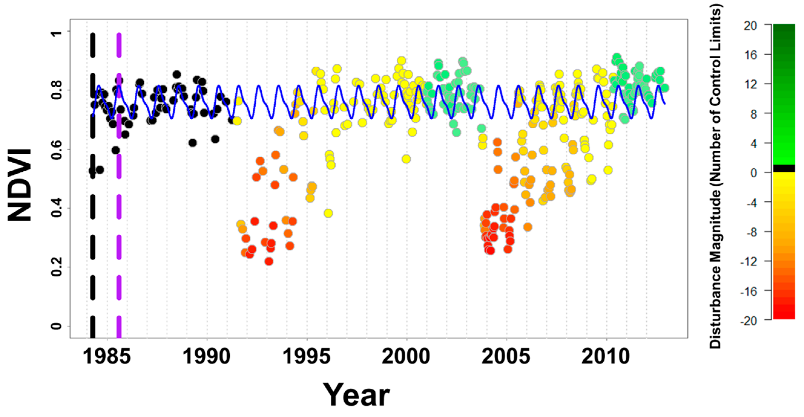
However, EWMACD continues to measure departures from the initial curve even after signaling a disturbance. While this can be helpful in comparing a pixel’s status from one time to the next, it does not effectively monitor the pixel’s trajectory in a continuous fashion [5]. For analyses spanning decades, a single training period is often insufficient to effectively capture forest change. Figure 1 offers an example of this problem. In this example, the pixel covers a pine forest plantation in North Carolina, USA, which exhibits a typical growth and harvest pattern. EWMACD is initialized during a condition of forest maturity, and it correctly signals the disturbance in 1991. However, it continues to treat the mature forest as the baseline for comparison, resulting in a consistent loss signal even when the forest clearly recovers; the pattern repeats for the disturbance in 2003–2004. While this example is not of a subtle disturbance, it does illustrate the problem associated with using a fixed reference curve.
Other contemporary change detection algorithms incorporate methods for long-term trend analysis. LandTrendr [7], ITRA (Image Trends from Regression Analysis) [8], VCT (Vegetation Change Tracker) [6], and VeRDET (Vegetation Regeneration and Disturbance Estimates through Time) [11] automatically target multi-year disturbances, but they do not directly use all available data and are constrained to an annual time step, which can reduce their ability to precisely identify disturbance timing. The Continuous Change Detection and Classification algorithm (CCDC) [9], an algorithm based on harmonic regression principles similar to those underlying EWMACD, has built-in methods for retraining curves and does use the full time series. However, CCDC is specifically focused on between-class changes and has difficulty signaling for “partially changed” pixels [9], the area in which EWMACD specializes.
Thus, what is needed is a dynamic update to EWMACD: an algorithm which can detect subtle forest disturbances in a long-term, flexible fashion. Accordingly, our objective is to present and assess Edyn (dynamic EWMACD), an EWMACD-based change detection algorithm that retrains its harmonic reference curves after a disturbance is registered. In this study we describe the differences between Edyn and EWMACD, then compare the two algorithms in an agreement assessment on over 3500 forested pixels from across the contiguous United States (CONUS) using decades-long time spans.
2. Materials and Methods
2.1. Reference Data and Spectral Data
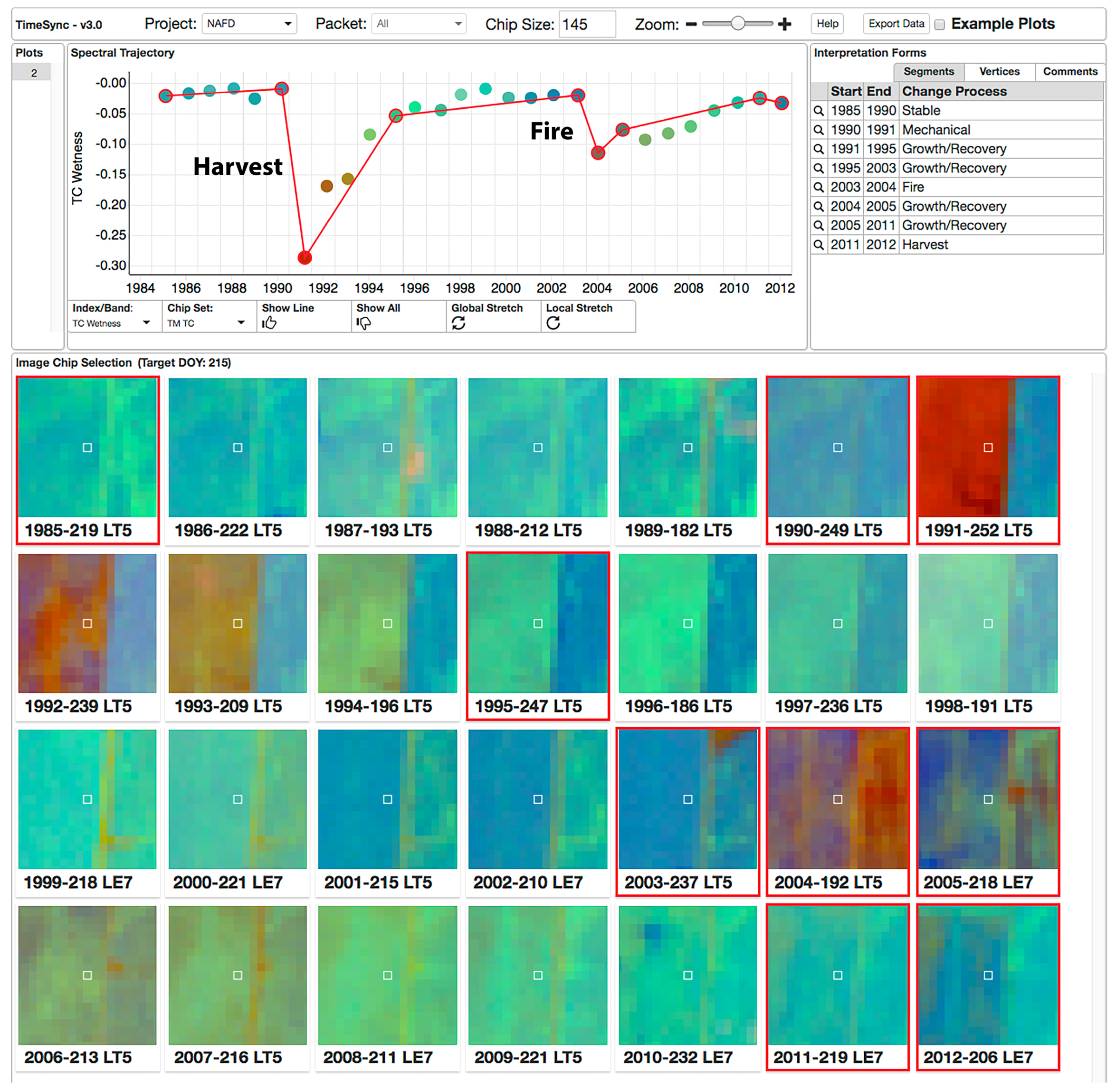
For reference data in our assessment, we used a collection of pixels interpreted by users of the TimeSync software [23], a web application hosted by Oregon State University. (TimeSync version 2.0 was used for generating the reference data.) These pixels were randomly sampled from a collection of 179 Landsat scenes covering a diverse subset of the CONUS ([13], Figure 1), with each scene hosting different forest types and disturbance regimes. Figure 2 shows the same pixel from Figure 1, when processed by TimeSync. All available Landsat images within the growing season (approximately May through October) were acquired for a 200 × 200-pixel area around each sample pixel. Each pixel’s time series was input into TimeSync and visually interpreted by a pair of expert analysts, with disagreements adjudicated by a third interpreter. For further information about the TimeSync process the reader is referred to [23]; for more on the reference dataset used in this study, please refer to [13].
For our study, we selected a subset of these reference data which corresponded to time series representing forested pixels. Typical timeframes ranged from 1985 to 2012, covering multiple Landsat sensors and platforms. Spectral data for each pixel were provided, as were data regarding the TimeSync disturbance interpretations. The dataset used in this study comprised 3751 pixels in total. We excluded all data marked by the associated Fmask codes [24] as non-clear, then computed NDVI (Normalized Difference Vegetation Index) values [25] for all remaining data to use as inputs to EWMACD and Edyn.
2.2. Review and Updates to EWMACD
While developing Edyn, we also updated EWMACD to improve general performance. A brief summary of the algorithm (Figure 3) and a description of these key modifications follows. For a full description of the original version of EWMACD, please refer to [5]. Vectors and matrices are in bold typeface; scalars are not.
Given an image time series of length , , and a corresponding Julian date time series , we first estimate harmonic coefficients for the first elements by ordinary least squares estimation using sine harmonics and cosine harmonics:
where is the design matrix consisting of a ones column and each harmonic adjustment to . In practice, we recompute after screening out all elements that have standardized residual values greater than a global, user-specifiable threshold. We then compute residuals for the full time series,
where is the full design matrix computed similarly. We then estimate the training period variance,
Next, we compute EWMA values for the full time series by setting and recursively calculating:
where is the smoothing parameter which indicates the weight of the current observation against the exponentially decayed weight of all prior observations. Note that we assume the mean of the in-control residuals (based on stable, undisturbed forest) to be 0, since OLS is an unbiased estimation technique.
At the same time, we compute signaling thresholds:
where (the control limit) determines how many standard deviations away from the in-control mean of 0 are required to signal. Then, we record the EWMACD outputs in relative form by dividing the EWMA values by the control limits and taking the floor of the absolute values multiplied by the original signs:
When the EWMA values extend beyond the signaling thresholds, EWMACD signals a disturbance; otherwise a value of 0 indicates no signaled disturbance. (The user can instead obtain an output of the raw EWMA chart values, if desired). Note that using this rule, EWMACD signals for both negative (e.g., removal) and positive (e.g., growth) deviations from the curve; EWMACD can be made to ignore positive deviations by setting the positive value of to infinity. EWMACD outputs correspond to each element of the input time series; thus they may be post-processed and summarized to give annual or similar summaries.
Parameter Updates
Many of the pre- and post-processing subroutines in EWMACD rely on a measure of persistence, defined here as a quantification of the number of consecutive elements in the time series that must occur before some decision is made (e.g., recording a signal as opposed to treating it as anomalous). This persistence was previously a global, user-specified parameter. However, due to inherently variable conditions and differences in image availability as functions of both time and location, the density of data for any given pixel or timeframe varies considerably. We therefore modified the persistence parameter into a persistence per year parameter, , allowing a user to specify what proportion of a year (or possibly multiple years) is considered to be “long enough” for the algorithm to act. Given this value, EWMACD now takes the mean number of elements per year in the time series, then modifies this value accordingly to obtain a per-pixel value for persistence. This value is thus data-driven yet more consistent with user expectations.
The quality of fit for the initial harmonic curve has a strong impact on EWMACD’s accuracy in general, making it important to have enough data to accurately and robustly fit this curve. Taking too little data into the training period risks overfitting and allowing the otherwise-unconstrained curves to deviate nonsensically [9,26,27], which can result in many false alarm signals when real data are compared to the extrapolations. On the other hand, taking too much data into the training period reduces the algorithm’s effectiveness by rendering a substantial portion of the time series unavailable for change detection, and doing so also increases the likelihood that the algorithm will attempt to train a curve on a disturbance. Thus, in an ideal situation EWMACD will take only the minimum amount of data required for an accurate curve-fitting. We achieve this by first determining a minimum training length of at least , where and are the number of harmonics for the sine and cosine terms being used in the Fourier expansion. Then, using a moving window starting at the beginning of the time series, the algorithm fits successive harmonic curves until it either achieves a minimum fit , denoted , or reaches the maximum training date (by default the point in the time series twice as large as the endpoint of the minimum training length), at which point it accepts the final curve. This process reduces the likelihood of training on a disturbance while ensuring that a well-fitted curve is found relatively early in the time series. Between specifying and , the user now has more flexible control over how likely EWMACD is to inadvertently train on a disturbance.
2.3. Edyn
When only a single disturbance occurs over a time series, EWMACD generally signals it and tracks the magnitude as it varies over time. This magnitude is valuable in its own right, as it is derived from the pixel’s trajectory and variability during the training period and in some sense incorporates that pixel’s unique characteristics as a result. Additionally, EWMACD is tuned to detect low-magnitude disturbances, as described in Section 2.2. Therefore, when determining when and how to retrain the harmonic curve after a signaled disturbance, we wanted to utilize this information and preserve the subtle change detection as much as possible.
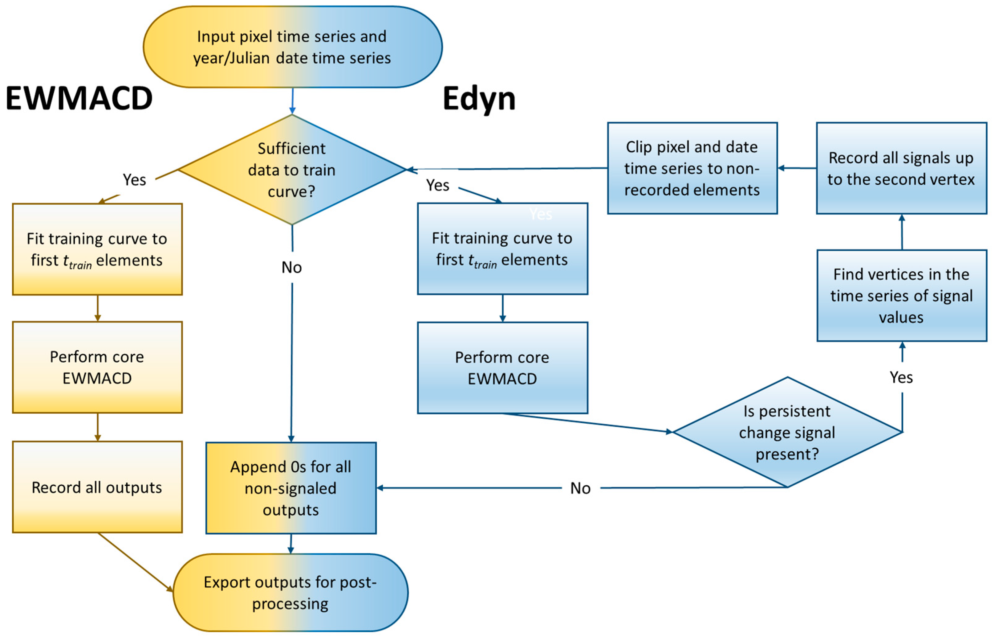
The workflow of the Edyn algorithm is given in Figure 4. Edyn initializes just as EWMACD does, with a harmonic curve fitted and EWMA values calculated to produce an output time series of signal values. However, when a disturbance is signaled, Edyn reinitializes on a subset of the original time series, restarting after the disturbance is presumed stabilized and recording the original outputs from the period before the new starting point. It then repeats the core EWMACD algorithm on the subset, reinitializing on further signals and repeating until either no disturbances are signaled or insufficient data remain. The resulting output is a spliced collection of EWMACD signal outputs, yielding a dynamic disturbance trajectory based on last-known-stable conditions.
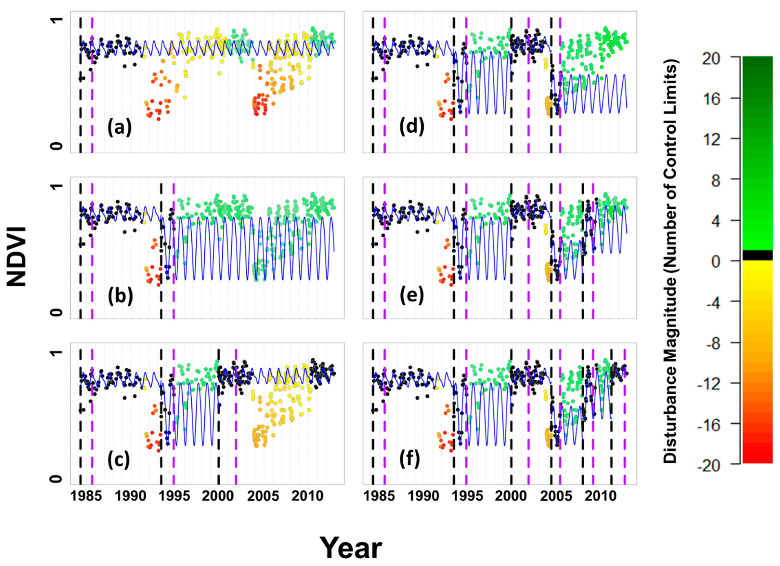
The crux of Edyn’s performance lies in accurately determining when a disturbance has stabilized. To do this, we make use of the previous EWMACD output as well as the persistence parameter and the training period demarcation, denoted here as , as follows. Given a time series of EWMACD outputs that signals a disturbance after the training period, we note that the outputs for the training period are assumed to be 0 (no change). Then, the first signaled disturbance represents a vertex in the output. However, simply reinitializing at this point would (1) most likely cause training on the continued disturbance or recovery thereof; or (2) cause the disturbance record to be overwritten as “retraining”. Therefore, we make the simplifying assumption that the second vertex in the signal time series represents the point at which the original disturbance has stabilized and the pixel has reached a new equilibrium, and we choose this point to reinitialize. Figure 5 illustrates this approach, using the same forested pixel shown in Figure 1 and Figure 2. Note that like EWMACD, Edyn signals for both negative and positive deviations from the curve by default.
We determine vertices in a manner similar to the methods used in LandTrendr [7], a segmentation-based change detection algorithm which inputs a time series (typically annual steps) and uses a sequence of linear interpolations to identify vertices. The segments defined by these vertices are then classified into disturbance, stable, and growth trends according to their slopes. In the case of Edyn, we find the line between the endpoints of a given segment, then find the point in the time series with the highest squared deviation from the line and designate it a vertex. We use this new vertex to partition the time series into two smaller ones and repeat, finding additional vertices. Candidate vertices are only considered if they are far enough away from previously identified vertices, using half the persistence value as the distance threshold (making a persistence-sized interval around a given vertex). The process is repeated until no more viable candidates can be found, at which point we identify the second vertex. Because EWMACD signals directly indicate observed changes, choosing this point generally ensures that the initial disturbance event is no longer active when retraining begins. Because EWMACD signals can capture subtle disturbances, they potentially offer more information than raw spectral or vegetation index values.
Figure 6 shows sample Edyn and EWMACD outputs for part of the study area of [5], a region of Alabama, USA that is dense in industrial pine plantations. In both cases, there is spatial coherence, indicating that both algorithms are likely capturing real change processes on the landscape, but note the stand in the north-central area, indicated by the arrow. Both algorithms signal a disturbance beginning in 2007. However, Edyn “resets” after a given time (the persistence: in this case, approximately one year’s worth of images) and ultimately signals growth in 2010–2011. EWMACD consistently signals the patch as a disturbance, although the degree does lessen from 2008 to 2011, as evidenced by the color shifting from reds to yellows. In both cases, the algorithms observe the disturbance, but they differ in how they quantify it.
2.4. Strengths and Limitations of EWMACD/Edyn
Like any change detection algorithm, EWAMCD and Edyn have both strengths and limitations that result from the underlying assumptions and model structure. Although it has not yet been employed across wide spatial extents, Edyn is based on the same core algorithm and thus shares many of the strengths and limitations of EWMACD, with the obvious exception being the ability to retrain its harmonic curves in support of long-term monitoring.
The most apparent strength of the two algorithms is their ability to detect subtle changes. EWMACD was shown to accurately detect forest thinning harvests in an industrial pine setting, including canopy reductions of as low as 25% based on visual inspection of aerial photographs [5]. EWMACD also detected stand-replacing disturbances with high accuracy, and the use of signal strength relative to pixel-specific control limits yielded maps which indicated both disturbance occurrence and relative magnitude, as well as direction (e.g., growth or removal). Furthermore, by using all available images instead of composites or annualized summaries, EWMACD signaled detected changes with good temporal precision, often signaling only one or two images after the disturbance occurred [5]. Finally, because the algorithms are defined generally, they can be employed on any remotely sensed time series regardless of land cover, sensor platform, or image frequency—provided sufficient data exist to train harmonic curves (two or three periods’ worth, as a rule of thumb).
However, this generality also underlies many of the algorithms’ limitations. EWMACD and Edyn are intended to detect and monitor change, but they are not in themselves designed to attribute such changes to particular causes (though their outputs could be used in an algorithm that does, such as that of [10] or [28]). The algorithms also rely on the harmonic curves for both the residual time series and the in-control statistics, so any pixel that normally exhibits non-harmonic patterns through time (e.g., vegetation in very arid climates) could confound the algorithms’ outputs. Similarly, a sparse time series for some pixels (e.g., from a cloud-covered rainforest) can lead to model overspecification, causing the in-control standard deviation estimate to be so small that the algorithms subsequently signal at the slightest fluctuation. In general, the algorithms’ focus on detecting subtle disturbances results in their being prone to larger commission error rates, as was seen in [14]. Finally, EWMACD/Edyn currently input a single spectral band or index at a time. While this may be sufficient for detecting typical changes in forests [29], in general the availability of multiple spectral bands represents a wealth of information that in many cases is already preprocessed and should be utilized. While rigorously adapting EWMACD/Edyn to a multiband input is outside the scope of the current study, we have already begun to do so.
2.5. Agreement Assessment
We used a simplified classification of disturbance to compare both EWMACD and Edyn against the TimeSync reference dataset. In particular, we computed EWMACD and Edyn outputs for NDVI time series derived from each of the 3751 forested pixels, using the full time series in each case and using the same default parameters given in Table 1. Note that our choice of the control limit, L, is slightly higher than the conventional value of [21]. We did this to better reflect the choice of parameters used in [14], as that study used similar reference data.
We summarized the Edyn/EWMACD outputs to an annual time step using a simple mean value per year approach. We then reclassified the annualized outputs into −1 (removal/decline) for negative values or 0 (no change/growth) for nonnegative values. Accordingly, any year in which a negative signal was generated for a given date would be a year in which the signal value was automatically −1. Similarly, we reclassified TimeSync segments into −1 and 0 and converted the TimeSync trajectories to annual timesteps and assigned the status from the corresponding segment to each year. For example, the pixel shown in Figure 2 had “Harvest” for 1990, “Growth/Recovery” for 1991–2003, and “Fire” for 2004, based on the corresponding TimeSync segment designations. We also preserved a simplified listing of disturbance agents as designated by TimeSync: Fire (4.4% of all annualized disturbances), Harvest (39.8%, including mechanical clearing), Stress (33.8%), and Other (21.9%, including wind, debris, water, and other agents which could not be attributed to another cause).
In general, disturbance of any type is a rare event [30]: across all forested TimeSync pixels and years, approximately 4% of the recorded values were disturbances, with 56% being no change and 40% being growth of some kind. This led us to use metrics which emphasize the algorithms’ ability to detect disturbances’ occurrence and timing within the general time series. In particular, we wanted to compare the overall disturbance record on a per-pixel basis, assessing whether the Edyn or EWMACD outputs successfully mimicked the TimeSync data in pattern as well as signal amounts. Thus, for each pixel we generated an error matrix for Edyn against the TimeSync data by treating each available year as a data point, then computed commission on disturbance (total false positive Edyn signals over all Edyn positive signals) and omission on disturbance (total false negative Edyn signals over all TimeSync positive signals). To assess general agreement between the time series, we also computed overall error (the false positive and false negative Edyn signals over all years). We performed the same process for EWMACD against TimeSync, generating in each case a collection of 3751 matched commission error, omission error, and overall error rates: one set per forested pixel.
To illustrate the error-generation process, some example pixels are given in Figure 7. For the case of low omission and high commission (Figure 7a), the NDVI series begins a decline circa 1990, with a minimum circa 1992 followed by a rise through the remainder of the 1990s. Edyn signals the initial decrease in 1990, one year ahead of TimeSync, but it continues to signal the disturbance through 2000 because the recovering NDVI trajectory does not level off sufficiently until that time. This results in a high commission error (82%) and a 0% omission error (since TimeSync never signals disturbance when Edyn does not). The failure of Edyn to retrain sooner in this example suggests a persistence value that was too high to capture the dynamic; it is notable that this occurred in the pre-Landsat 7 era, when the data density was lower. In Figure 7b, the NDVI time series is relatively stable to visual inspection, with a slight decrease over 2000–2006. TimeSync signals the beginning of this decrease but not the end; Edyn signals the end (including 2007) but not the beginning, yielding a 100% commission error and a 100% omission error. In the case of Figure 7c, both Edyn and TimeSync signal a single-year disturbance in 2004 corresponding to a clear drop in the NDVI time series, resulting in 0% commission and 0% omission errors for Edyn. Finally, in the case of high omission and low commission (Figure 7d), the original training data from 1984 to 1986 are noisy. Due to its burn-in period, Edyn has no chance to signal the disturbance registered by TimeSync in those years but fits a curve around the stable portion of the data. However, the resultant high in-control SD dulls the algorithm’s sensitivity for the remainder of the time series, causing it to also miss the slight decreases to NDVI in 1996 and 2001–2002. These four examples, while by no means exhaustive, do illustrate possible causes of disagreement between Edyn and the TimeSync data and highlight the need for caution when interpreting the results.
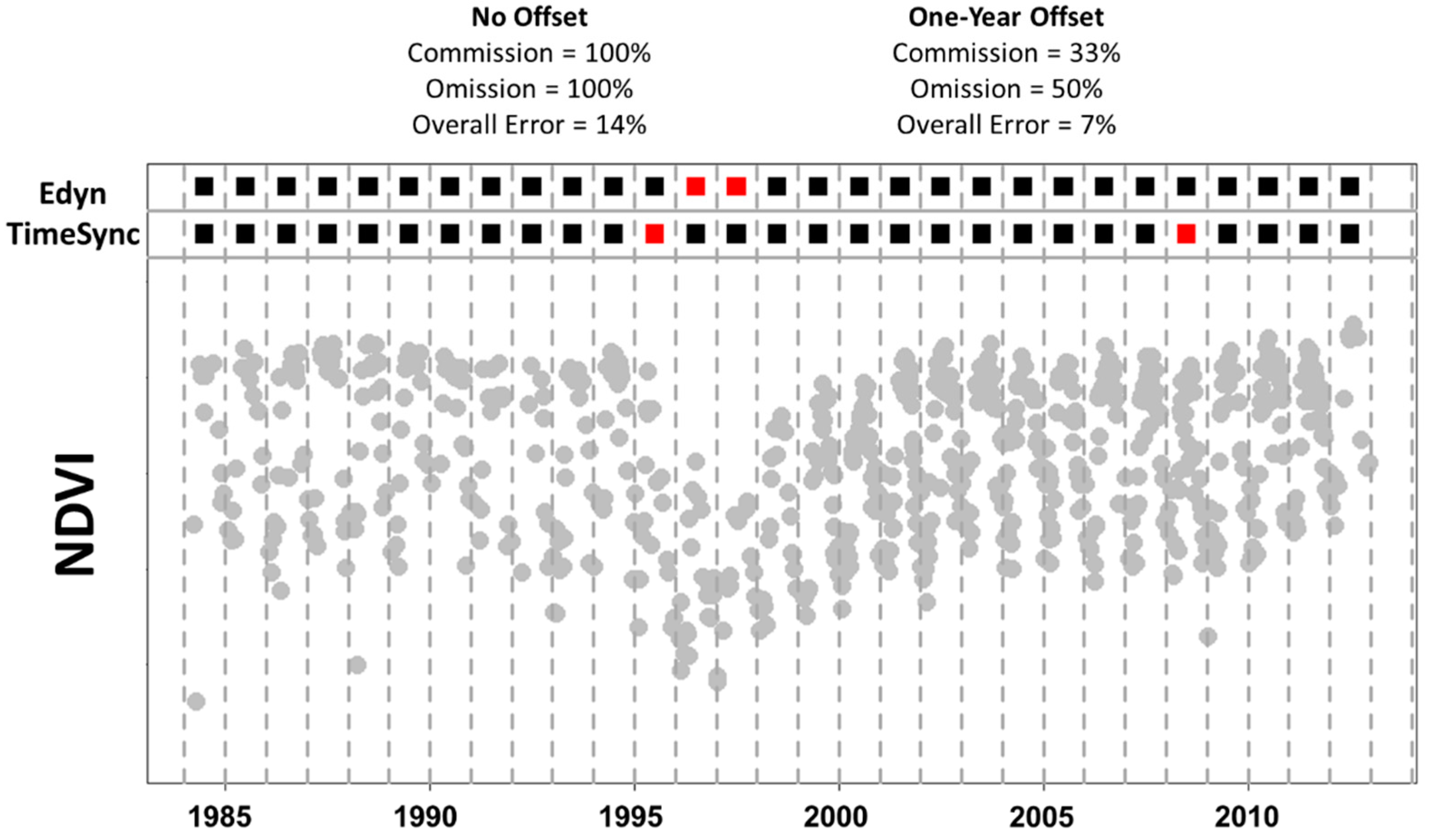
This approach to calculating error did not allow for timing disagreements; however, it was not uncommon to have pixels for which both Edyn and TimeSync were signaling the same disturbance but disagreed on the exact timing and duration. Figure 8 provides an example of this case: under the strict year-by-year method, the resultant 100% commission and omission error rates do not offer any numerical evidence that the two time series were clearly signaling the same basic disturbance in 1995–1996. As such disagreements could be explained by noting that Edyn could begin signaling at any date within the year (and thus a single-year signal could be stretched over two years, as seems to be the case in mid-1995 through mid-1996), we additionally generated a set of more flexible signal time series by allowing a potential one-year offset on signaled disturbances to improve matching. Using this rule, the signal time series in Figure 8 would be adjusted so that the TimeSync signal in 1995 would count as an agreed disturbance with Edyn by virtue of the Edyn signal in 1996, while the Edyn signal in 1997 would still count as commission error because there was no TimeSync signal recorded in 1996–1998. Similarly, the TimeSync signal in 2008 still generates an omission error for Edyn, as there were no Edyn signals in 2007–2009. Using these “blurred” time series, we computed per-pixel error matrices as before and generated collections of commission, omission, and overall error rates, noting that such error rates may be biased to smaller values by virtue of “double-counting” overlapped years of agreement.
We made the error comparison for all 3751 forested pixels in the reference data, but we were also interested in particular subsets relating to Edyn’s ability to detect various types of disturbances. In particular, we assessed agreement for pixels which included at least one TimeSync disturbance (1620 pixels). We also partitioned this into the subset of forested pixels for which the disturbing agent was not stress (1408 pixels) as well as considering the case where the disturbing agent was stress (212 pixels), as Edyn and EWMACD are specifically designed to detect subtle, persistent changes.
In all cases, we considered the distributions of the errors of commission and omission on disturbance, as well as overall error against the TimeSync data. To complement the commission, omission and overall error rates, we also computed the F1 score (or balanced F score):
where precision is the complement of commission error and recall is the complement of omission error. This score is a single-number summary of accuracy that treats omission and commission as being equally important. Finally, in each case we compared the error rates from Edyn and EWMACD using paired t-tests to assess whether the difference in algorithm performance was statistically significant. Results are presented separately for the no-offset and one-year temporal offset groups.
3. Results
The main results of the agreement assessment are shown in Table 2. Differences in the mean error rates between Edyn and EWMACD were generally significant, with the only exceptions being the commission and overall error rates for the stress-only subset, most likely due to a small relative difference and a relatively small sample size.
In general, Edyn had lower per-pixel rates of commission error than EWMACD, and in general Edyn had higher per-pixel rates of omission error. Since Edyn retrains the harmonic curves after a disturbance, it might reasonably be expected to have a lower commission error than EWMACD, as it will no longer signal “outdated” disturbances (as in Figure 1). Similarly, because it removes data to achieve retraining, it is reasonable to expect Edyn to also have a higher omission error rate, as years during such retraining are treated as non-disturbed. Edyn also exhibited lower overall error rates than EWMACD in every case (albeit less so for stressed forested pixels), which suggests that it is more faithfully mimicking the TimeSync data by virtue of its retraining. Allowing for a one-year offset in disturbance timing decreased the error rates in all cases and all subsets, but the overall pattern remained the same.
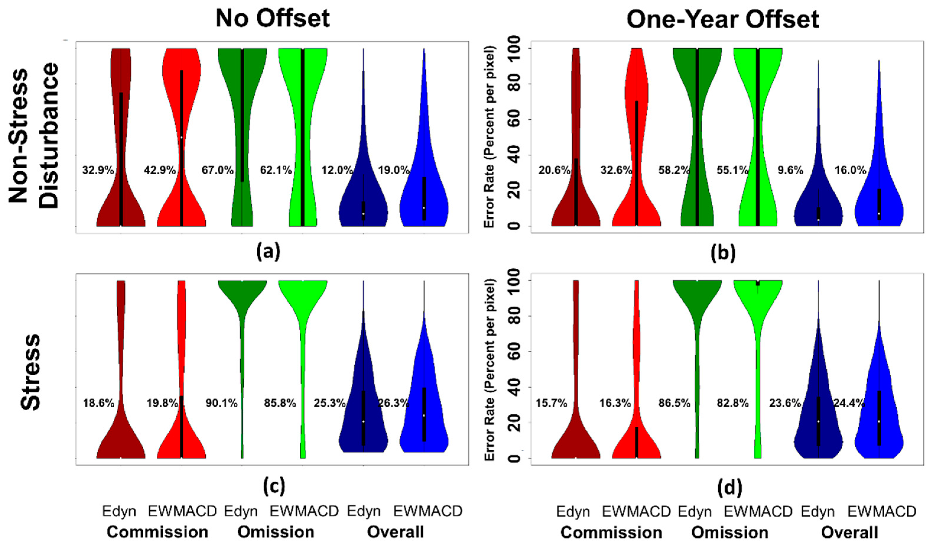
Because disturbance-based error rates depend greatly on the number of disturbance signals in a given time series, we also considered the distribution of the error rates, in this case the commission on disturbance, omission on disturbance, and overall disagreement between the algorithm and TimeSync data. Figure 9 shows such distributions in the form of violin plots, in this case for disturbed forests pixels excluding stress and stressed forested pixels with no timing offset (Figure 9a,b) and the same when allowing a one-year timing offset (Figure 9c,d). From the figures it is clear that the commission and omission error rates are generally bimodally distributed, with distinct subsets of pixels for which there were either very high or very low error rates. Given that a commission (or omission) error of 100% can easily be achieved by mismatching a single year in an otherwise stable trajectory, the plots illustrate the importance of interpreting the error rates carefully. It is interesting to note that allowing the one-year offset reduced the non-stress commission and omission errors more than for the stressed forested pixels subset; this is most likely due to the acute nature of many such disturbances (e.g., harvest or fire) and justifies the use of the offset to compensate for algorithmic differences in disturbance timing. Finally, the overall error rate in each plot is generally clustered around small values, suggesting that per-time-series agreement between both Edyn and EWMACD, as compared to the TimeSync data, was relatively good.
Since Edyn and EWMACD offer signals for both disturbance timing and severity, we also further analyzed the distribution of their disagreements with TimeSync by binning them into severity classes (Severe, Moderate, Subtle, No Signal and Growth) based on the observed relative magnitude of NDVI change (in signal thresholds) signaled by the algorithms (Table 3). We did this on an annualized basis, not on a per-pixel basis, so there was no offset to consider here. We found that for both algorithms, omission errors were higher in the Stress category than for all other types of disturbance, while the magnitudes for correctly signaled stress were generally in the Subtle category, both of which are to be expected given the low magnitude of change and general detection difficulty associated with stress [12,13,14,15]. However, EWMACD misclassifies almost twice as many stressed years as being growth years compared to Edyn (13.6% versus 7.8%), suggesting that the Edyn signals, when available, are generally better at detecting stress than the EWMACD signals. Importantly, when excluding the no-signal bin, Edyn had a general omission error rate of 19.2%, less than the omission error rate of 26.9% for EWMACD. While we did not explicitly filter out the exact years in which Edyn retrained, this reversal of the usual omission rate pattern in Table 2 strongly suggests that when these retraining periods are excluded, Edyn agrees with TimeSync more than EWMACD does.
Based on the consistency of the results, we conclude that Edyn generally performed better than EWMACD in terms of overall agreement and lower commission error for forested pixels. EWMACD still outperformed Edyn in terms of omission error rates, but this appears to be largely a reflection of the opportunity costs of retraining the harmonic curves for Edyn. This cost may be compensated by the generally higher accuracy Edyn exhibited in detecting disturbances while not retraining.
4. Discussion
Several questions and caveats arise from the study presented here, some of which may prove fruitful avenues for future work. A brief discussion of these points follows.
There are fundamental differences in the way TimeSync and Edyn handle spectral data. Most importantly, the analysts developing the TimeSync reference data utilized all spectral bands and numerous indices for the images. As currently designed, Edyn inputs one band or index. This increases processing speed but fails to take full advantage of all available data. For example, in Figure 7d we observed TimeSync signaling a disturbance where Edyn did not. Visual inspection of the NDVI time series offers only vague intuition that a disturbance has occurred, but further inspection of the short-wave infrared band time series revealed distinct vertices at the associated year. Without using these other bands there is no way for Edyn to detect this disturbance, short of training a curve so tightly that even the slightest deviation would trigger a signal. Thus, there is certainly incentive to develop a multi-band approach based on the assumptions underlying Edyn; EWMACD could similarly be modified.
Conversely, we must note that while the TimeSync data were used here as a reference, they are also subject to error. Sun et al. [31] found that while mutual visual interpretation can produce consistent results among the interpreters, that in itself is no guarantee of accuracy. In general, the relative unavailability of ground truth data (which also contains errors, even discounting the differences due to top-down and bottom-up perspectives), particularly historical ground truth data, continues to impact the community’s ability to assess the accuracy of time series-based approaches. This can be alleviated for more recent historical periods as the era of big data and frequent measurements begins, but the issue will continue to remain a challenge for long-term studies.
Another important potential issue arises from the nature of the data set and the persistence-per-year parameter, . In computing it as the mean number of data points (available images) per year for a given pixel, we are assuming a certain regularity in data frequency. However, the data frequency doubled in 1999 with the establishment of Landsat 7. Thus, Edyn/EWMACD may have treated the 1983–1999 period differently from the 1999–2012 period. We saw an example of this in Figure 7a. It is possible that establishing two persistence parameters, or dividing a 1999-present value by 2, could mitigate this if a user finds problems as a result of the divide.
The error rates reported in the agreement assessment are generally lower than those reported in [14], which made a general comparison between seven change detection algorithms—CCDC [9], LandTrendr [7], ITRA [8], MIICA (Multi-Index Integrated Change Analysis) [32], VCT [6], VeRDET [11], and the then-current version of EWMACD—across a sample of 1800 pixels drawn from six Landsat scenes across the CONUS. There, EWMACD was seen to have commission and omission rates of approximately 80% and 70%, respectively. The difference lies in part in the methods for computing error. In [14], a generalized error matrix was created, summing all yearly agreements/disagreements over all pixels before computing the error rates. In this study, we summed yearly disagreements for each pixel independently and computed error on a per-pixel basis because we were also interested in the algorithms’ ability to mimic the overall time series patterns observed in the TimeSync data, including non-disturbance pattern and timing. Thus we also performed an agreement assessment using such a generalized error matrix, finding that for all forested pixels Edyn had commission and omission error rates of 86.1% and 77.0%, respectively, while EWMACD had error rates of 89.5% (commission) and 71.9% (omission) when using no offset allowance. When a one-year offset was allowed, Edyn had error rates of 72.0% commission and 57.6% omission, while EWMACD had 78.0% commission and 50.8% omission. This suggests again that a considerable number of omission errors were in actuality one-year timing disagreements between Edyn/EWMACD and TimeSync. In any case, the pattern of results—Edyn having fewer commission errors and better overall agreement with TimeSync while having more omission errors than EWMACD—remained the same. Finally, we also made a direct comparison with the algorithms in [14] by implementing Edyn and EWMACD using the same data and methods from that study, where possible using the same input parameters as were used for EWMACD there. Compared to the other algorithms, Edyn had the fourth lowest general commission rate and the fourth lowest general omission rate; EWMACD had the fifth lowest commission rate and the second lowest omission rate. Partitioning agreement by the disturbance agents used in [14] (Table 4), we found that for the subset of forested pixels in decline, both Edyn and EWMACD had lower rates of omission error than almost every other algorithm [14] (Table 3), with the exceptions of the previous version of EWMACD and LandTrendr. The discrepancy in EWMACD results can be explained by new parameters such as ; LandTrendr had the advantage of being similar in nature to the TimeSync reference data with which it was being compared, as both rely on temporal segmentation of annual time series [7,23].
A natural question that arises from this study is whether there is a condition or circumstance in which a user might prefer EWMACD over Edyn—or more generally, when an algorithm that uses a fixed reference might be preferable to one that updates such references. To answer this, we note that while Edyn had better overall agreement with TimeSync than EWMACD did, this agreement reflects the time series-based approach to error calculation. This in turn places assumed value on the algorithms’ ability to mirror the full time series, including time steps with no disturbance. Reconsidering Figure 1 and Figure 5, if the question of interest relied on comparing status between two points in time, EWMACD might be the more appropriate choice between the two because it maintains the initial baseline. A user could simply initialize EWMACD at the “before” time and run until the “after” time, as in [5]. In fact, based on the observed high omission error rates, using Edyn may cause the user to completely miss changes of interest if it happens to be retraining during the second timeframe.
Ultimately, when discussing change detection and accuracy, one must be careful to precisely define what “change” is. Current state-of-the-art change detection algorithms are tested according to their creators’ and users’ needs, and a great many are specialized to particular use cases. These algorithms can often be used on general image stacks, but it is essential to understand their intended uses and keep their underlying assumptions in mind when doing so. For example, despite their generality in accepting input data, Edyn and EWMACD were designed for use on vegetated pixels assumed to exhibit some degree of harmonic variation throughout the year. The algorithms will yield results for other types of pixels, but those results may be unintuitive or easily misinterpreted.
Given the sheer number of change detection algorithms available today, there is incentive and potential benefit to designing algorithms to fill certain niches, not only to help distinguish them for the end user but also to aid ensemble efforts that seek to leverage algorithm differences to improve results, as in [33,34]. As an example, while the high omission error rates for stress in the agreement assessment indicate ample remaining room for improvement, both Edyn and EWMACD returned lower omission error rates for decline than all but one other algorithm from [14] in direct comparison. Thus, while they by no means captured the subtle, persistent disturbances in the reference data as hoped for, they at least were relatively good at doing so among contemporary change detection algorithms.
5. Conclusions
In this study we found that Edyn agreed better with the TimeSync reference data than EWMACD did, with a mean disagreement rate of 13.7% (Table 2) when considering a binary disturbance/non-disturbance case for disturbed forested pixels, compared to 19.9% for EWMACD. When allowing a one-year offset for timing discrepancies on this subset, Edyn had a mean overall disagreement rate of 8.2%, still smaller than 14.0% for EWMACD. We also found that Edyn generally yielded lower rates of commission error on disturbances, while it yielded higher rates of omission error.
Edyn and EWMACD will continue to be freely available and open-source [19], and they will be usable for any remotely sensed time series with sufficient temporal data. The results of this study show that Edyn represents a small improvement over its parent algorithm, EWMACD, in terms of long-term subtle disturbance detection, though we note that the relatively small sample size of 212 pixels is insufficient to make a robust claim. Nevertheless, it is our hope that as end users continue to monitor the landscape for long-term changes, they now have an additional tool to utilize.
Acknowledgments
This work was supported in part by the RPA Land Use Modeling Grant/Contract ID 14-JV-11330145-108, funded by the USDA Forest Service; the Pine Integrated Network: Education, Mitigation, and Adaptation Project (PINEMAP), a Coordinated Agricultural Project funded by the US Department of Agriculture (USDA) National Institute of Food and Agriculture (NIFA), Award No. 2011-68002-30185; and the US Geological Survey Grant G12PC00073, “Making Multitemporal Work”. Funding for R.H.W.’s and V.A.T.’s participation was also provided in part by the Virginia Agricultural Experiment Station and the McIntire-Stennis Program of NIFA, USDA (Project Number 1007054, “Detecting and Forecasting the Consequences of Subtle and Gross Disturbance on Forest Carbon Cycling”). Funding for Z.Y.’s participation was provided through the Landscape Change Monitoring System (LCMS) funded by the USDA Forest Service. The costs for publishing in open access were discounted by institutional membership with MDPI through the Virginia Tech library. The authors thank the anonymous reviewers for their insightful feedback on the original manuscript.
Author Contributions
E.B.B., V.A.T. and R.H.W. conceived the study; Z.Y. provided the TimeSync reference data; E.B.B. created the algorithm, assisted by V.A.T. and R.H.W.; E.B.B. designed and coordinated the study; E.B.B. and Z.Y. performed the accuracy assessment; E.B.B. led the writing, assisted by V.A.T., R.H.W. and Z.Y.
Conflicts of Interest
The authors declare no conflict of interest. The funding sponsors had no role in the design of the study; in the collection, analyses, or interpretation of data; in the writing of the manuscript, or in the decision to publish the results.
References
- Cohen, W.B.; Goward, S.N. Landsat’s role in ecological applications of remote sensing. BioScience 2004, 54, 535–545. [Google Scholar] [CrossRef]
- Hansen, M.C.; Loveland, T.R. A review of large area monitoring of land cover change using Landsat data. Remote Sens. Environ. 2012, 122, 66–74. [Google Scholar] [CrossRef]
- Hirschmugl, M.; Gallaun, H.; Dees, M.; Datta, P.; Deutscher, J.; Koutsias, N.; Schardt, M. Methods for mapping forest disturbance and degradation from optical earth observation data: A review. Curr. For. Rep. 2017, 3, 32–45. [Google Scholar] [CrossRef]
- Potapov, P.V.; Turubanova, S.A.; Hansen, M.C.; Adusei, B.; Broich, M.; Altstatt, A.; Mane, L.; Justice, C.O. Quantifying forest cover loss in Democratic Republic of the Congo, 2000–2010, with Landsat ETM+ data. Remote Sens. Environ. 2012, 122, 106–116. [Google Scholar] [CrossRef]
- Brooks, E.B.; Wynne, R.H.; Thomas, V.A.; Blinn, C.E.; Coulston, J.W. On-the-fly massively multitemporal change detection using statistical quality control charts and Landsat data. IEEE Trans. Geosci. Remote Sens. 2014, 52, 3316–3332. [Google Scholar] [CrossRef]
- Huang, C.; Goward, S.N.; Masek, J.G.; Thomas, N.; Zhu, Z.; Vogelmann, J.E. An automated approach for reconstructing recent forest disturbance history using dense Landsat time series stacks. Remote Sens. Environ. 2010, 114, 183–198. [Google Scholar] [CrossRef]
- Kennedy, R.E.; Yang, Z.; Cohen, W.B. Detecting trends in forest disturbance and recovery using yearly Landsat time series: 1. LandTrendr—Temporal segmentation algorithms. Remote Sens. Environ. 2010, 114, 2897–2910. [Google Scholar] [CrossRef]
- Vogelmann, J.E.; Xian, G.; Homer, C.; Tolk, B. Monitoring gradual ecosystem change using Landsat time series analyses: Case studies in selected forest and rangeland ecosystems. Remote Sens. Environ. 2012, 122, 92–105. [Google Scholar] [CrossRef]
- Zhu, Z.; Woodcock, C.E. Continuous change detection and classification of land cover using all available Landsat data. Remote Sens. Environ. 2014, 144, 152–171. [Google Scholar] [CrossRef]
- Moisen, G.G.; Meyer, M.C.; Schroeder, T.A.; Liao, X.; Schleeweis, K.G.; Freeman, E.A.; Toney, C. Shape selection in Landsat time series: A tool for monitoring forest dynamics. Glob. Chang. Biol. 2016, 22, 3518–3528. [Google Scholar] [CrossRef] [PubMed]
- Hughes, M.; Kaylor, S.; Hayes, D. Patch-based forest change detection from Landsat time series. Forests 2017, 8, 166. [Google Scholar] [CrossRef]
- McDowell, N.G.; Coops, N.C.; Beck, P.S.A.; Chambers, J.Q.; Gangodagamage, C.; Hicke, J.A.; Huang, C.Y.; Kennedy, R.; Krofcheck, D.J.; Litvak, M.; et al. Global satellite monitoring of climate-induced vegetation disturbances. Trends Plant Sci. 2015, 20, 114–123. [Google Scholar] [CrossRef] [PubMed]
- Cohen, W.B.; Yang, Z.; Stehman, S.V.; Schroeder, T.A.; Bell, D.M.; Masek, J.G.; Huang, C.; Meigs, G.W. Forest disturbance across the conterminous United States from 1985–2012: The emerging dominance of forest decline. For. Ecol. Manag. 2016, 360, 242–252. [Google Scholar] [CrossRef]
- Cohen, W.; Healey, S.; Yang, Z.; Stehman, S.; Brewer, C.; Brooks, E.; Gorelick, N.; Huang, C.; Hughes, M.; Kennedy, R.; et al. How similar are forest disturbance maps derived from different Landsat time series algorithms? Forests 2017, 8, 98. [Google Scholar] [CrossRef]
- Neigh, C.S.R.; Bolton, D.K.; Williams, J.J.; Diabate, M. Evaluating an automated approach for monitoring forest disturbances in the Pacific Northwest from logging, fire and insect outbreaks with Landsat time series data. Forests 2014, 5, 3169–3198. [Google Scholar] [CrossRef]
- Kurz, W.A.; Dymond, C.C.; Stinson, G.; Rampley, G.J.; Neilson, E.T.; Carroll, A.L.; Ebata, T.; Safranyik, L. Mountain pine beetle and forest carbon feedback to climate change. Nature 2008, 452, 987–990. [Google Scholar] [CrossRef] [PubMed]
- Running, S.W. Climate change—Ecosystem disturbance, carbon, and climate. Science 2008, 321, 652–653. [Google Scholar] [CrossRef] [PubMed]
- Seidl, R.; Schelhaas, M.J.; Rammer, W.; Verkerk, P.J. Increasing forest disturbances in Europe and their impact on carbon storage. Nat. Clim. Chang. 2014, 4, 806–810. [Google Scholar] [CrossRef] [PubMed]
- Exponentially Weighted Moving Average Change Detection—Script and Sample Data. Available online: https://vtechworks.lib.vt.edu/handle/10919/50543?show=full (accessed on 2 June 2017).
- Raza, S.M.M.; Siddiqi, A.F. EWMA and DEWMA control charts for poisson-exponential distribution: Conditional median approach for censored data. Qual. Reliab. Eng. Int. 2017, 33, 387–399. [Google Scholar] [CrossRef]
- Reynolds, M.R.; Stoumbos, Z.G. Comparisons of some exponentially weighted moving average control charts for monitoring the process mean and variance. Technometrics 2006, 48, 550–567. [Google Scholar] [CrossRef]
- Woodall, W.H.; Mahmoud, M.A. The inertial properties of quality control charts. Technometrics 2005, 47, 425–436. [Google Scholar] [CrossRef]
- Cohen, W.B.; Yang, Z.; Kennedy, R. Detecting trends in forest disturbance and recovery using yearly Landsat time series: 2. TimeSync—Tools for calibration and validation. Remote Sens. Environ. 2010, 114, 2911–2924. [Google Scholar] [CrossRef]
- Zhu, Z.; Woodcock, C.E. Object-based cloud and cloud shadow detection in Landsat imagery. Remote Sens. Environ. 2012, 118, 83–94. [Google Scholar] [CrossRef]
- Tucker, C.J. Red and photographic infrared linear combinations for monitoring vegetation. Remote Sens. Environ. 1979, 8, 127–150. [Google Scholar] [CrossRef]
- Brooks, E.B.; Thomas, V.A.; Wynne, R.H.; Coulston, J.W. Fitting the multitemporal curve: A fourier series approach to the missing data problem in remote sensing analysis. IEEE Trans. Geosci. Remote Sens. 2012, 50, 3340–3353. [Google Scholar] [CrossRef]
- Hermance, J.F. Stabilizing high-order, non-classical harmonic analysis of NDVI data for average annual models by damping model roughness. Int. J. Remote Sens. 2007, 28, 2801–2819. [Google Scholar] [CrossRef]
- Schroeder, T.A.; Schleeweis, K.G.; Moisen, G.G.; Toney, C.; Cohen, W.B.; Freeman, E.A.; Yang, Z.Q.; Huang, C.Q. Testing a Landsat-based approach for mapping disturbance causality in U.S. forests. Remote Sens. Environ. 2017, 195, 230–243. [Google Scholar] [CrossRef]
- Zhu, Z.; Woodcock, C.E.; Olofsson, P. Continuous monitoring of forest disturbance using all available Landsat imagery. Remote Sens. Environ. 2012, 122, 75–91. [Google Scholar] [CrossRef]
- Masek, J.G.; Goward, S.N.; Kennedy, R.E.; Cohen, W.B.; Moisen, G.G.; Schleeweis, K.; Huang, C.Q. United States forest disturbance trends observed using Landsat time series. Ecosystems 2013, 16, 1087–1104. [Google Scholar] [CrossRef]
- Sun, B.; Chen, X.; Zhou, Q. Analyzing the uncertainties of ground validation for remote sensing land cover mapping in the era of big geographic data. In Spatial Data Handling in Big Data Era; Zhou, C., Su, F., Harvey, F., Xu, J., Eds.; Springer Nature: Singapore, 2017; pp. 31–38. [Google Scholar]
- Jin, S.; Yang, L.; Danielson, P.; Homer, C.; Fry, J.; Xian, G. A comprehensive change detection method for updating the National Land Cover Database to circa 2011. Remote Sens. Environ. 2013, 132, 159–175. [Google Scholar] [CrossRef]
- Healey, S.P.; Cohen, W.B.; Zhiqiang, Y.; Brewer, C.K.; Brooks, E.B.; Gorelick, N.; Hernandez, A.J.; Huang, C.; Hughes, M.J.; Kennedy, R.E.; et al. Mapping forest change using stacked generalization: An ensemble approach. Remote Sens. Environ. 2017. in review. [Google Scholar]
- Saxena, R.; Watson, L.T.; Wynne, R.H.; Thomas, V.A. Scaling constituent algorithms of a trend and change detection polyalgorithm. In Proceedings of the 2017 Spring Simulation Multi Conference on High Performance Computing Symposium, Virginia Beach, VA, USA, 23–26 April 2017. [Google Scholar]
Figure 1.
EWMACD (Exponentially Weighted Moving Average Change Detection) outputs based on an NDVI (Normalized Difference Vegetation Index) time series for an example pixel covering a planted pine stand. The blue line represents the baseline fitted harmonic curve from which residuals are taken. Black and purple dashed vertical lines demarcate the beginning and ending of the curve’s training period, respectively. The algorithm successfully signals the disturbances in 1991 and 2003–2004, but it is unable to detect the subsequent regrowth from either because it continues to use the original training curve. The disturbance magnitude represents the distance of the EWMACD signals from 0 (stable) in units of control limits (the signaling threshold for the underlying exponentially weighted moving average chart).

Figure 2.
TimeSync interpretation of the pine forest pixel from Figure 1, covering the same time span. Note the signaled disturbances in 1991 and 2004, similar to Figure 1.

Figure 3.
Core EWMACD process for a given pixel/time series.
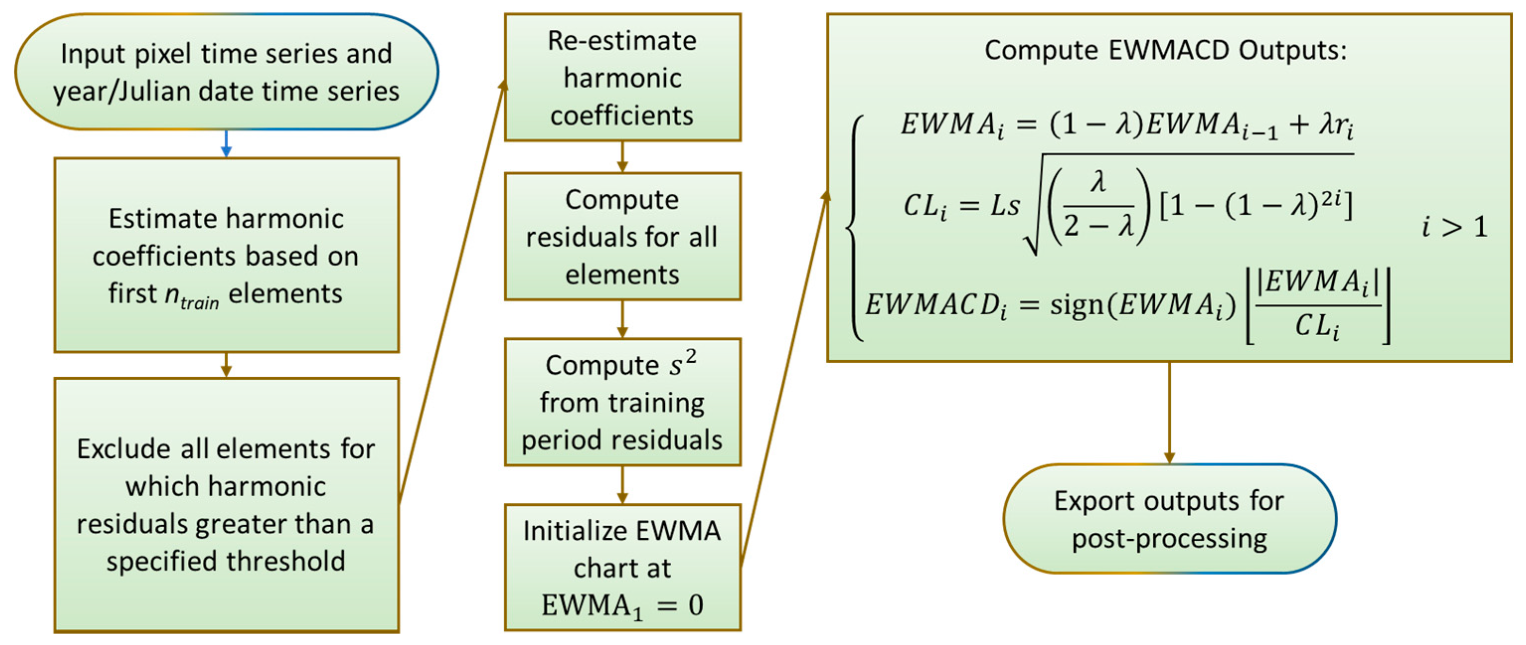
Figure 4.
Workflow for EWAMCD and Edyn algorithms. Complete details for core EWMACD processing can be found in Brooks et al., 2014 [5]; a brief description can be found in Section 2.2 and Figure 3.
Figure 4.
Workflow for EWAMCD and Edyn algorithms. Complete details for core EWMACD processing can be found in Brooks et al., 2014 [5]; a brief description can be found in Section 2.2 and Figure 3.

Figure 5.
Edyn algorithm, step by step, using the same forested pine pixel from Figure 1 and Figure 2. (a) The first pass of the algorithm is identical to a normal EWMACD run (the blue curve is the harmonic fit and the black and purple lines demarcate the beginning and end of the curve training period); (b) the second pass retrains the harmonic curve after the initial disturbance (in this case in 1991) is determined to have stabilized; (c–f) subsequent passes continue until no further signals are detected or insufficient training data remain.

Figure 6.
Edyn and EWMACD outputs for a subset of the study area in central Alabama, USA from Brooks et al., 2014 [5]. Note the north-central patch (indicated by the arrows) as an example of Edyn retraining reference curves.
Figure 6.
Edyn and EWMACD outputs for a subset of the study area in central Alabama, USA from Brooks et al., 2014 [5]. Note the north-central patch (indicated by the arrows) as an example of Edyn retraining reference curves.
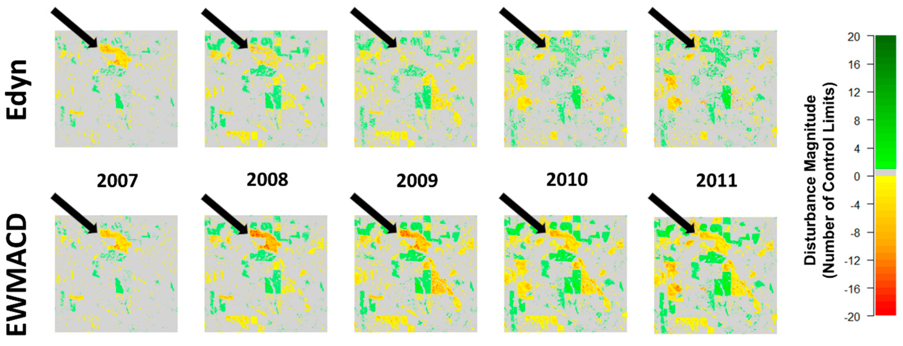
Figure 7.
Commission and omission errors for Edyn against the TimeSync reference data, for four example pixels. NDVI (gray) time series and disturbance (red)/non-disturbance (black) signals are given for each, with Edyn above the corresponding TimeSync signals. Error rates are given as well. (a) High commission and low omission; (b) high commission and high omission; (c) low commission and low omission; (d) low commission and high omission.
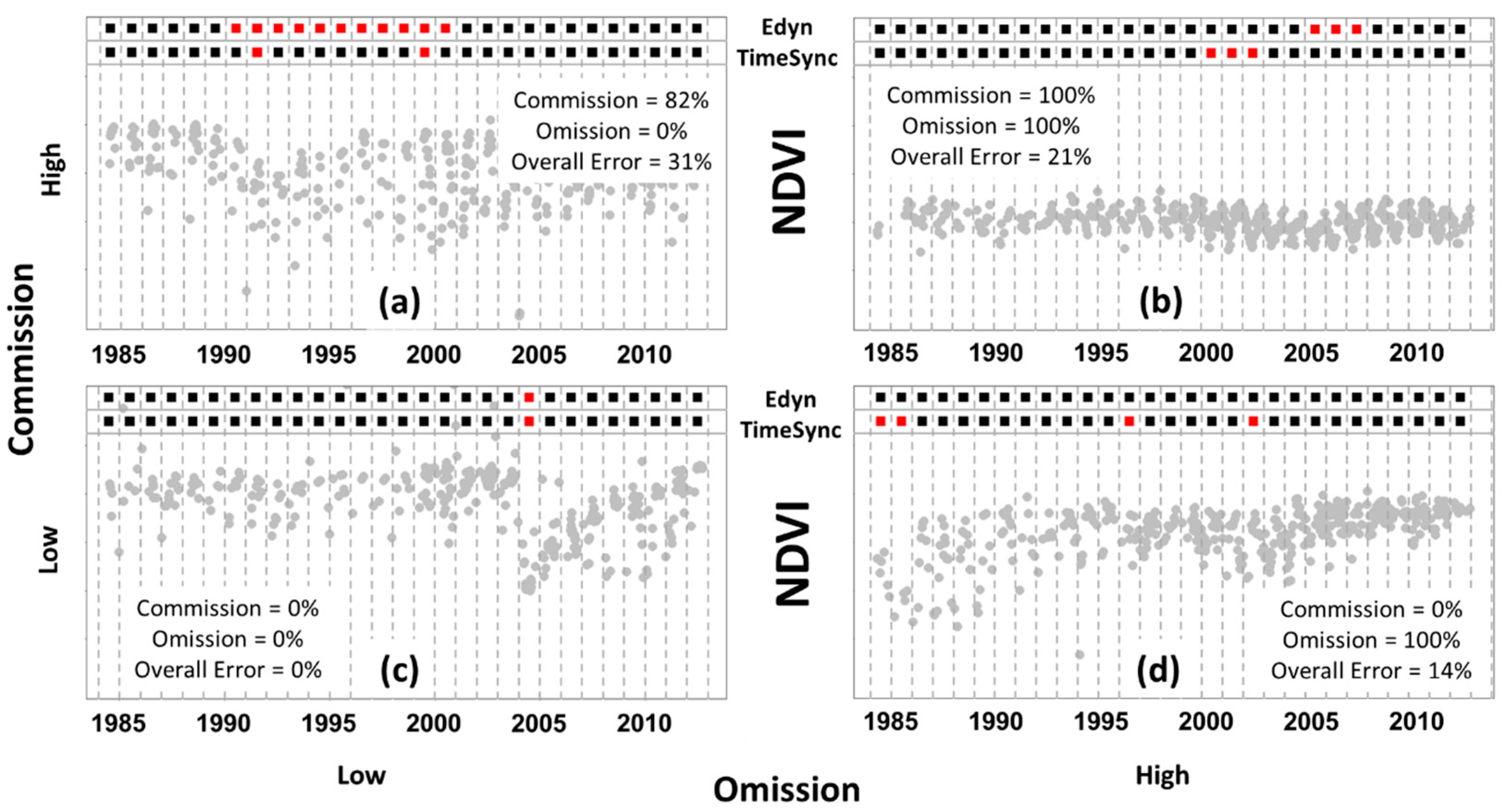
Figure 8.
Effect of the one-year offset on error rates of Edyn and TimeSync algorithms, for an example time series (29 years). Note that the offset “extends” the disturbance signal for a given year if and only if there is a pre-existing disturbance signal from the other data source within one year.
Figure 8.
Effect of the one-year offset on error rates of Edyn and TimeSync algorithms, for an example time series (29 years). Note that the offset “extends” the disturbance signal for a given year if and only if there is a pre-existing disturbance signal from the other data source within one year.

Figure 9.
Violin plots of the commission, omission and overall error rates for the subsets of (a) disturbed forested pixels excluding stress with no timing offset (1408 pixels); (b) disturbed forested pixels excluding stress with a one-year offset (1408 pixels); (c) stressed forested pixels with no timing offset (212 pixels); and (d) stressed forested pixels with a one-year offset (212 pixels). Mean errors are listed to the left of each violin. Note the bimodal distributions for the commission and omission error rates, as well as the decrease in commission and omission errors for non-stressed forest pixels when allowing the one-year offset.

Table 1.
Selected parameters for Edyn/EWMACD used in this study.
| Parameter | Description | Value |
|---|---|---|
| Smoothing parameter; weight of current observation against prior history | 0.3 | |
| Control limit; number of standard deviations away from 0 required to signal | 5 | |
| Proportion of a typical year desired to designate “consistent” change | 1 | |
| Number of cosine and sine harmonics used in the curve-fitting, respectively | 2, 2 | |
| Minimum required to accept harmonic curve | 0.7 |
Table 2.
Mean error rates and F1 scores for Edyn and EWMACD outputs compared as time series against various subsets of the TimeSync reference data. Mean error rates when allowing a one-year offset are given in parentheses below the associated results. Pairings with significantly different mean error rates are marked by an asterisk.
| Pixel Subset | Total Pixels | Commission | Omission | Overall Error | F1 Score | ||||
|---|---|---|---|---|---|---|---|---|---|
| Edyn | EWMACD | Edyn | EWMACD | Edyn | EWMACD | Edyn | EWMACD | ||
| All Forested Pixels | 3751 | 20.6% * (15.8% *) | 24.0% * (19.9% *) | 34.6% * (26.7%*) | 32.5% * (25.4% *) | 7.8% * (6.7% *) | 11.1% * (9.7% *) | 0.54 * (0.63 *) | 0.52 * (0.60 *) |
| Disturbed Forested Pixels | 1620 | 31.1% * (19.9% *) | 39.9% * (30.4% *) | 70.0% * (61.9% *) | 65.2% * (58.7% *) | 13.7% * (11.4% *) | 19.9% * (17.1% *) | 0.19 * (0.30 *) | 0.13 * (0.23 *) |
| Disturbed Forested Pixels (No Stress) | 1408 | 32.9% * (20.6% *) | 42.9% * (32.6% *) | 67.0% * (58.2% *) | 62.1% * (55.1% *) | 12.0% * (9.6% *) | 19.0% * (16.0% *) | 0.21 * (0.33 *) | 0.13 * (0.25 *) |
| Disturbed Forested Pixels (Stress Only) | 212 | 18.60% −15.70% | 19.80% −16.30% | 90.1% * (86.5% *) | 85.8% * (82.8% *) | 25.30% −23.60% | 26.30% −24.40% | 0.09 −0.12 | 0.1 −0.13 |
Table 3.
Edyn/EWMACD signal magnitudes for forested pixels by TimeSync disturbance class, year-by-year. Note that an Edyn value of 0 can also indicate that it is retraining the reference curve. Percentages sum to 100% row-wise, within reference disturbance classes: for example, omission error rates may be derived for the disturbance classes by summing the No signal and Growth percentages within each row (except for Stable and Recovery).
| TimeSync Disturbance Class | Severe [−20, −3) | Moderate [−3, −1) | Subtle [−1, 0) | No signal [0, 1) | Growth [1, 20] |
|---|---|---|---|---|---|
| Edyn | |||||
| All Disturbances | 172 (4.4%) | 371 (9.5%) | 393 (10.1%) | 2734 (70.2%) | 223 (5.7%) |
| Fire | 13 (7.5%) | 37 (21.4%) | 24 (13.9%) | 92 (53.2%) | 7 (4.0%) |
| Harvest | 89 (5.7%) | 195 (12.5%) | 200 (12.9%) | 987 (63.6%) | 80 (5.2%) |
| Other | 67 (7.8%) | 99 (11.6%) | 91 (10.7%) | 564 (66.0%) | 33 (3.9%) |
| Stress | 3 (0.2%) | 40 (3.0%) | 78 (5.9%) | 1091 (83.0%) | 103 (7.8%) |
| Stable | 151 (0.2%) | 735 (1.2%) | 1715 (2.8%) | 54,113 (89.1%) | 4031 (6.6%) |
| Recovery | 285 (0.7%) | 952 (2.2%) | 1623 (3.7%) | 34,232 (78.9%) | 6300 (14.5%) |
| EWMACD | |||||
| All Disturbances | 325 (8.3%) | 464 (11.9%) | 360 (9.2%) | 2321 (59.6%) | 423 (10.9%) |
| Fire | 38 (22.0%) | 44 (25.4%) | 18 (10.4%) | 56 (32.4%) | 17 (9.8%) |
| Harvest | 146 (9.4%) | 210 (13.5%) | 172 (11.1%) | 838 (54.0%) | 185 (11.9%) |
| Other | 120 (14.1%) | 122 (14.3%) | 83 (9.7%) | 487 (57.0%) | 42 (4.9%) |
| Stress | 21 (1.6%) | 88 (6.7%) | 87 (6.6%) | 940 (71.5%) | 179 (13.6%) |
| Stable | 340 (0.6%) | 1052 (1.7%) | 2243 (3.7%) | 50,608 (83.3%) | 8103 (10.7%) |
| Recovery | 934 (2.2%) | 1755 (4.0%) | 2825 (6.5%) | 29,775 (68.6%) | 6502 (18.7%) |
Table 4.
Annualized disturbance/non-disturbance Edyn/EWMACD agreement with TimeSync for the 1800 pixels used in Cohen et al., 2017 [14], partitioned across TimeSync disturbance classes. Direct comparison may be made to Table 3 of [14].
| Algorithm Signal | Not Disturbed | Harvest | Fire | Decline | Wind | Other | All Disturbances |
|---|---|---|---|---|---|---|---|
| Edyn | |||||||
| Not Disturbed | 30,208 | 406 | 30 | 890 | 43 | 146 | 1515 |
| Disturbed | 1713 | 234 | 24 | 114 | 18 | 60 | 450 |
| Omission | N/A | 63.4% | 55.6% | 88.6% | 70.5% | 70.9% | 77.1% |
| EWMACD | |||||||
| Not Disturbed | 28,388 | 401 | 19 | 823 | 42 | 132 | 1417 |
| Disturbed | 3533 | 239 | 35 | 181 | 19 | 74 | 548 |
| Omission | N/A | 62.7% | 35.2% | 82.0% | 68.9% | 64.1% | 72.1% |
© 2017 by the authors. Licensee MDPI, Basel, Switzerland. This article is an open access article distributed under the terms and conditions of the Creative Commons Attribution (CC BY) license (http://creativecommons.org/licenses/by/4.0/).
Share and Cite
MDPI and ACS Style
Brooks, E.B.; Yang, Z.; Thomas, V.A.; Wynne, R.H. Edyn: Dynamic Signaling of Changes to Forests Using Exponentially Weighted Moving Average Charts. Forests 2017, 8, 304. https://doi.org/10.3390/f8090304
AMA Style
Brooks EB, Yang Z, Thomas VA, Wynne RH. Edyn: Dynamic Signaling of Changes to Forests Using Exponentially Weighted Moving Average Charts. Forests. 2017; 8(9):304. https://doi.org/10.3390/f8090304
Chicago/Turabian StyleBrooks, Evan B., Zhiqiang Yang, Valerie A. Thomas, and Randolph H. Wynne. 2017. "Edyn: Dynamic Signaling of Changes to Forests Using Exponentially Weighted Moving Average Charts" Forests 8, no. 9: 304. https://doi.org/10.3390/f8090304
Note that from the first issue of 2016, this journal uses article numbers instead of page numbers. See further details here.