Vertical Ozone Gradients above Forests. Comparison of Different Calculation Options with Direct Ozone Measurements above a Mature Forest and Consequences for Ozone Risk Assessment

Abstract

The estimation of the ozone (O₃) stomatal dose absorbed by a forest is a crucial step for O₃ risk assessment. For this purpose, data on O₃ concentrations at the forest top-canopy are needed. However, O₃ is barely measured at that height, while more often it is measured at a lower height above a different surface, typically a grassland near to the forest edge. The DO3SE model for O₃ stomatal flux calculation estimates the top-canopy O₃ concentration in near neutral stability conditions. However, near-neutrality is quite rare in the field, particularly in southern Europe. In this work, we present a modification of the DO3SE gradient calculation scheme to include the atmospheric stability. The performance of the new calculation scheme was tested against the direct measurements above a mature forest. Different gradient estimation options were also tested and evaluated. These options include simplified gradient calculation schemes and the techniques of the tabulated gradients described in the UN/ECE Mapping Manual for O₃ risk assessment. The results highlight that the inclusion of the atmospheric stability in the DO3SE model greatly improves the accuracy of the stomatal dose estimation. However, the simpler technique of the tabulated gradients had the best performance on a whole-season time frame.

1. Introduction

It has been reported that ozone levels have increased in the last decades both in rural and urban areas [1] while ozone peak values have decreased. Ozone negative effects on forest trees have been reported in a number of experimental trials (e.g., [2,3]) as well as in field observations (e.g., [4,5]).

The estimation of the accumulated ozone dose absorbed by a forest is a crucial step in every ozone risk assessment procedure. For this reason, ozone concentration just at the top of the forest canopy is needed. However, very few O₃ concentrations are measured at that height and more often they are measured at a lower height above a different surface, typically a grassland outside the forest edge where the meteorological station is located.

Above and below any measuring point over a vegetated surface, ozone shows a vertical gradient. This gradient, common to every scalar, assumes a typical logarithmic shape described by the Monin–Obukhov similarity theory (MOST), with a minimum ozone concentration near the vegetated surface and an increasing ozone concentration departing vertically from it.

The magnitude of this increase depends on several factors related to the characteristics of the surface (e.g., the geometry of the canopies and canopy shading [6]), to the rate of O₃ consumption by vegetation (through stomatal uptake and non-stomatal deposition) and soil [7], to the in-canopy chemical reactions [8,9] and to the stability conditions of the atmosphere as discussed, e.g., in Tuovinen and Simpson (2008) [10].

However, it is worth reiterating that the logarithmic shape of the gradient profiles predicted by the MOST should be regarded as a theoretical idealization. In the real world, many scalars measured in forest canopies may not exhibit MOST style decay, for example, when chemical reactions take place [9].

Moreover, the requirements of MOST are not always met in plant canopies, despite the ubiquitous application of this theory. These requirements include, e.g., the stationarity of scalars, the absence of sources and sinks between the measuring height and the exchanging surface, and the horizontal homogeneity of the underlying surface which fails when forest edges are present [11]. The reader can refer to Finnigan [12] and Katul et al. [13] for a complete critical review.

The direct consequence of the existence of an ozone gradient above the vegetation is that the direct use of the concentrations measured above the vegetation (Figure 1A) without any gradient correction will lead to an overestimation of the exposure and phytotoxic dose.

The situation is even more complicated when no measurements at all are available from above the forest top-canopy, and only measurements taken at the standard height (2 m) of a nearby automatic air quality monitoring station can be accessible. This latter is by far the most common situation, and is well represented in Figure 1B [14].

In this case, measurements at 2–5 m above the ground may underestimate ozone concentration at the top of the forest canopy (Figure 1B).

To cope with this problem, the DO3SE (Deposition of Ozone for Stomatal Exchange) model [15], which is widely used to estimate the stomatal ozone fluxes to vegetation across Europe, implemented a methodology to estimate the top-forest O₃ concentration based on the MOST. This methodology, firstly outlined by Tuovinen et al. [14], is partially described in the Mapping Manual of the CLRTAP (Convention on Long-Range Transboundary Air Pollution) of the UN/ECE (The United Nations Economic Commission for Europe) [16] and assumes the near neutrality atmospheric stability condition, which is very rare in field conditions, particularly in southern Europe.

In this work, we present a modification of the DO3SE gradient calculation scheme to explicitly account for the different atmospheric stability conditions, as introduced by Tuovinen and Simpson [10]. For this purpose, the similarity functions Ψ_M and Ψ_H [17] and the stability parameter L (Monin–Obukhov length) have been introduced in the equations to calculate the atmospheric resistance to ozone R_a and the friction velocity u*. Then, we extended the calculation scheme for the estimation of the top-canopy ozone concentration over a forest to the case in which the ozone concentrations are measured on a grassy area apart from the target forest. Furthermore, we tested the performance of the new calculation scheme by comparing the calculated top-canopy O₃ concentrations with real data, i.e., with the ozone concentrations directly measured above a mature forest during the whole year 2013.

The calculations were made on the ozone concentrations and meteorological measurements at 2 m a.g.l. (above ground level), available from an air quality monitoring station. This monitoring station was located above a short grass field, a few kilometers upwind of the forest edge, in an area where the ozone concentration field is homogeneous [18].

Different gradient estimation options with increasing levels of data input requirements were tested and evaluated. These options included simplified gradient calculation schemes and the techniques of the tabulated gradients described in the UN/ECE Mapping Manual for ozone risk assessment [16].

The consequences of these gradient calculation methods on the estimation of the ozone stomatal dose taken up by the forest were assessed by comparing the calculated Phytotoxic Ozone Dose (POD) with the O₃ stomatal flux derived from direct eddy covariance measurements performed above the forest top-canopy.

2. Materials and Methods

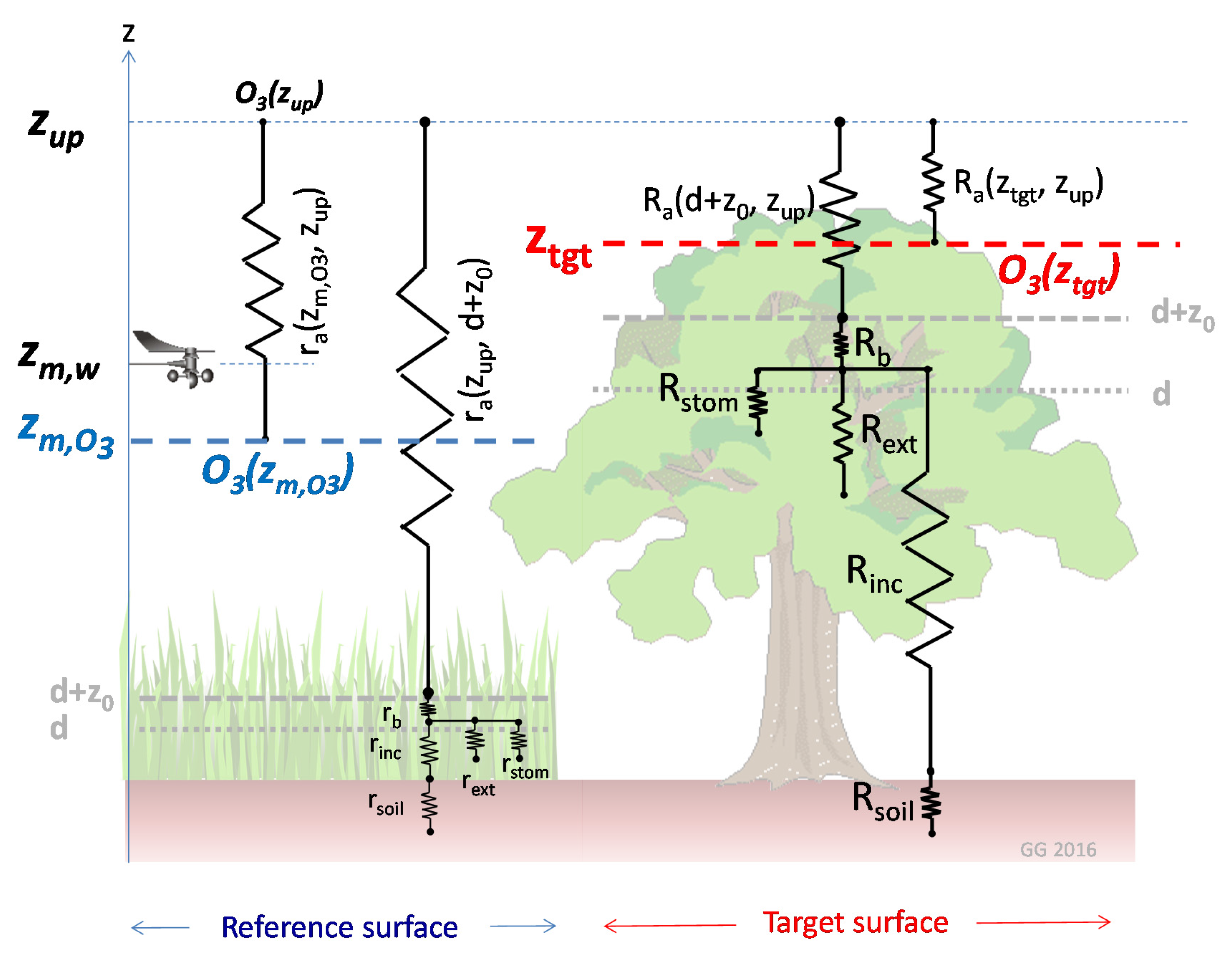
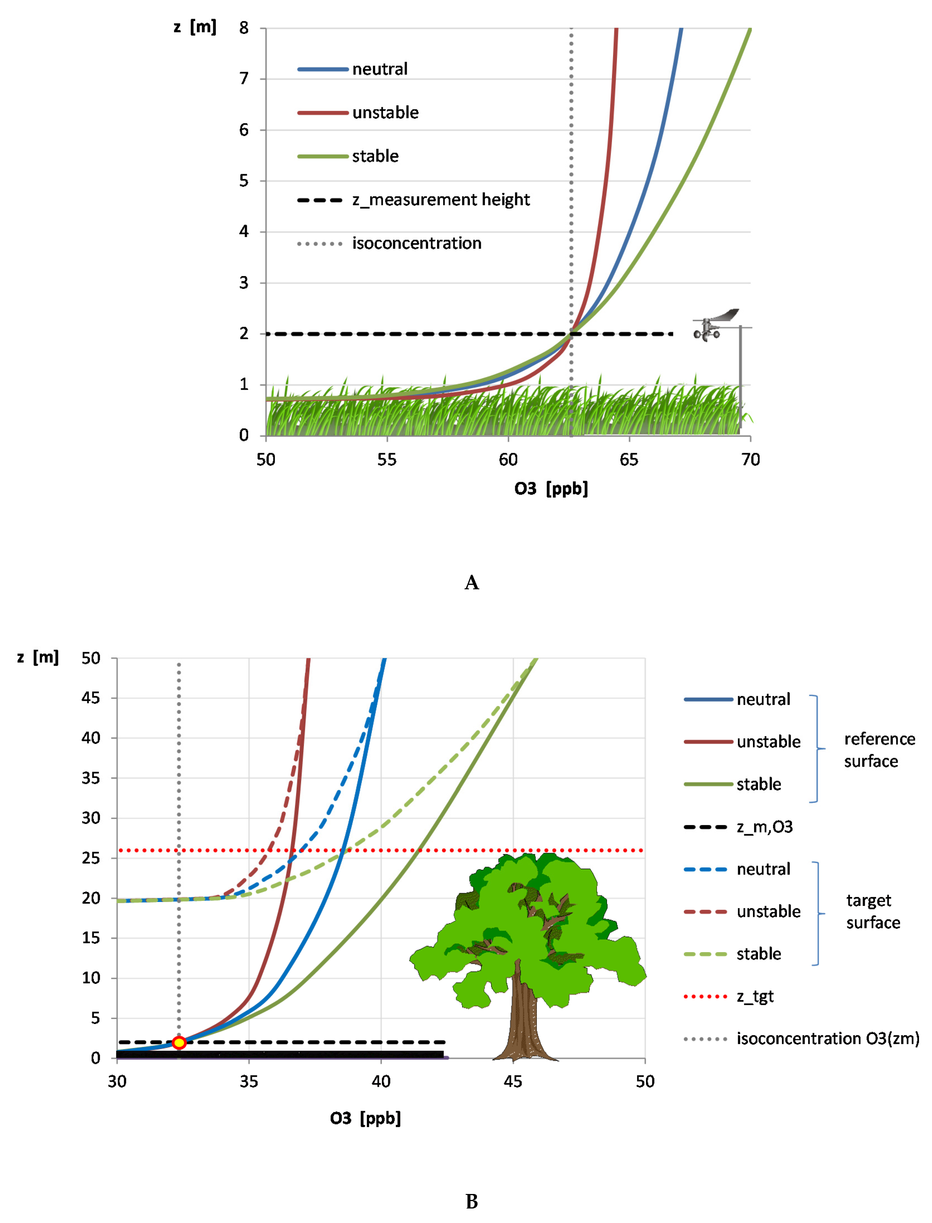
2.1. Estimation of Ozone Concentrations at the Top of the Forest Canopy from Measurements Taken above a Nearby Short Grassland

Ozone concentrations measured over a short grassland were used to estimate the O₃ concentrations at a reference height greater than the forest height, and then the appropriate gradient profile for the forest surface was applied to derive the concentrations at the top of the forest canopy.

The situation is described in Figure 2, where O₃(z_m,O3) and u(z_m,O3) are the ozone concentration and the wind speed measured over the grassland (hereafter called reference surface) at the measuring heights z_m,O3 and z_m,w respectively. The aerodynamic features of the reference surface have been reported in

Table 1. Parameters used for the gradient calculation exercise. For the meaning of the parameters listed in the section ‘Stomatal conductance’ of the Table, please refer to the Mapping Manual UN/ECE [16].

Geometry	Grassland (Reference surface)		Forest (Target surface)
Canopy height	href	0.05 m	htgt	26 m
Displacement height	dref	0.035 m	dtgt	18.2 m
Roughness length	z0,ref	0.005 m	z0,tgt	2.6 m
Leaf Area Index	LAI	3.5	LAI	3.5
Surface Area Index	SAI	3.5	SAI	4.5
[O3] measuring height	Zm,O3	2 m
Wind speed measuring height	Zm,w	2 m
Target height for [O3] calc.			ztgt	24 m
Decoupling height	zup	50 m
Constant Resistances
Cuticular resistance to O3 dep.	rext	2500 s/m	Rext	2500 s/m
Soil resistance to O3 dep.	rsoil	200 s/m	Rsoil	200 s/m
Stomatal Conductance (gs)
Maximum gs to H2O	gmax,H20	270 mmol m−2 s−1	gmax,H20	230 mmol m−2 s−1
Fmin	fmin	0.01	fmin	0.06
fPAR	alight	0.009	alight	0.003
fT	Tmin	12 °C	Tmin	0 °C
	Topt	26 °C	Topt	20 °C
	Tmax	40 °C	Tmax	35 °C
	b	1	b	0.75
fVPD	VPDmax	1.3 KPa	VPDmax	1.0 KPa
	VPDmin	3.0 KPa	VPDmin	3.25 KPa
fSWP	SWPmin	−1.5 MPa	SWPmin	−1.2 MPa
	SWPmax	−0.49 MPa	SWPmax	−0.5 MPa
fPHEN	SGS	1 DOY	SGS	105 DOY
	fphen_1	0 days	fphen_1	20 days
	fphen_4	0 days	fphen_4	30 days
	fphen_a	1	fphen_a	0
	fphen_e	1	fphen_e	0
	EGS	365 DOY	EGS	297 DOY
Soil Water
Soil type	Clay-loam		Clay-loam
Water content at field capacity	SWCfc	0.37 m3/m3	SWCfc	0.37 m3/m3
Water content at wilting point	SWCwp	0.1676 m3/m3	SWCwp	0.1676 m3/m3
	Ψe	−0.00588 MPa	Ψe	−0.00588 MPa
	bsoil	7	bsoil	7
Root depth	rdepth	0.80 m	rdepth	1.00 m

while the calculation of all the resistances to ozone deposition over the reference surface (r_a, r_b, r_stom, r_ext, r_inc, r_soil) will be described below. Table 1 reports also the aerodynamic features of the target surface (e.g., forest). The resistances to ozone deposition over the forest (R_a, R_b, R_stom, R_ext, R_inc, R_soil) will be also described below.

The ozone concentration at the top of the forest canopy (the target height z_tgt) was obtained with the big-leaf model approximation [6] and the constant-flux assumption [5] for the definition of the aerodynamic resistances. In the following, the roughness sub-layer affecting the concentration profiles near the canopy top was neglected, but a method for correcting the roughness sub-layer can be found in [10]. Moreover, extensive homogeneous surfaces (i.e., an adequate fetch) were assumed and the measurements used were not taken too close to the forest edge [14].

As a first step, the ozone concentration was calculated at the height z_up, which is not influenced by variation in the properties of the underlying surface. This height was assumed to be 50 m [19] and it is consistent with the outputs of the EMEP (European Monitoring and Evaluation Program) Chemical Transport Model [10] which feeds the DO3SE model.

The O₃ concentration at the height z_up is given by:

$$O_3\left(z_{up}\right)=\frac{O_3\left(z_{m,O3}\right)}{1-\frac{r_a\left(z_{m,O3}, z_{up}\right)}{r_a\left(d_{ref}+z_0, z_{up}\right)+r_b+r_{surf}}}$$

(1)

where $O_3\left(z_{m,O3}\right)$ is the available ozone measurement above the grassland canopy; $r_a\left(z_{m,O3},z_{up}\right)$ is the aerodynamic resistance between the height where ozone was measured and the height z_up; $r_a\left(d_{ref}+z_0,z_{up}\right)$ is the aerodynamic resistance to ozone deposition, i.e., the atmospheric resistance between the height z_up and the height of the upper boundary of the laminar sub-layer of the theoretical big-leaf surface which represents the grassland; r_b is the resistance to ozone diffusion in the laminar sub-layer; and r_surf is the overall resistance to ozone deposition, to the grassland leaves and the underlying soil. The latter includes the stomatal resistance to ozone uptake r_stom, the resistance of the external cuticles r_ext, the soil resistance to ozone deposition r_soil and the air resistance to ozone transfer within the vegetation layer r_inc.

The two atmospheric resistances are given by the following expressions:

$$r_a\left(z_{m,O3}, z_{up}\right)=\frac{1}{k·u_{ref}^{*}}\left[\ln \left(\frac{z_{up}-d_{ref}}{z_{m,O3}-d_{ref}}\right)-{\Psi }_H\left(\frac{z_{up}-d_{ref}}{L}\right)+{\Psi }_H\left(\frac{z_{m,O3}-d_{ref}}{L}\right)\right]$$

(2)

$${\mathit{r}}_a\left(d_{ref}+z_0, z_{up}\right)=\frac{1}{k·u_{ref}^{*}}\left[\ln \left(\frac{z_{up}-d_{ref}}{z_{0,ref}}\right)-{\Psi }_H\left(\frac{z_{up}-d_{ref}}{L}\right)+{\Psi }_H\left(\frac{z_{0,ref}}{L}\right)\right]$$

(3)

with $u_{ref}^{*}$ the friction velocity above the reference surface calculated as follows

$$u_{ref}^{*}=\frac{k·u\left(z_{m,w}\right)}{\ln \left(\frac{z_{m,w}-d_{ref}}{z_{0,ref}}\right)-{\Psi }_M\left(\frac{z_{m,w}-d_{ref}}{L}\right)+{\Psi }_M\left(\frac{z_{0,ref}}{L}\right)}$$

(4)

where k is the von Kármán constant (=0.41 [20]); $u\left(z_{m,w}\right)$ is the wind speed measured at the height z_m,w; d_ref is the displacement height assumed as two-thirds of the canopy height; z_0,ref is the roughness length assumed as 1/10 of the canopy height; and ${\Psi }_M(.)$ is the integral form of the similarity function for momentum which takes into account the stability of the atmospheric surface layer in terms of the Obukhov length L (1/L approaches zero if the atmosphere is neutral, 1/L < 0 if the atmosphere is unstable, 1/L > 0 if the atmosphere is stable) [17].

Taking the adimensional length $\zeta$ as argument, the function ${\Psi }_M(\zeta )$ is defined by the formulation of Garratt [17]:

$${\Psi }_M\left(\zeta \right)=\{\begin{array}{ll}\ln [\frac{1+x^2}{2}·{\left(\frac{1+x}{2}\right)}^2]-2\arctan (x)+\frac{\pi }{2},& when \zeta <0\\ -5\zeta ,& when \zeta \ge 0\end{array}$$

(5)

with $x={\left(1-16·\zeta \right)}^{1/4}$.

Instead, the ${\Psi }_H(.)$ function which appears in Equations (2) and (3) is the similarity function for heat defined by Garratt [17] as:

$${\Psi }_M\left(\zeta \right)=\{\begin{array}{ll}2\ln \left[\frac{1+x^2}{2}\right],& when \zeta <0\\ -5,& when \zeta \ge 0\end{array}$$

(6)

with x as defined in Equation (5).

The Obukhov length needed to account for the atmospheric stability is defined as in [21]:

$$L=-\frac{u_{*}^3}{k \frac{g}{T}\frac{H}{\rho c_p}}$$

(7)

where u* is the friction velocity (m/s), k is the Von Kármán constant (0.41, adim), g is the gravity acceleration (9.8 m s⁻²), T is the air temperature (K), H is the sensible heat flux (W m⁻²), ρ is the air density (kg m⁻³), c_p is the specific heat at constant pressure (1048 J kg⁻¹ K⁻¹).

The values of u* and H for the calculation of L can be obtained from eddy covariance measurements (see the following Section 2.2) or L can be estimated from standard meteorological measurements by following the procedure illustrated in Appendix A.

The resistance to ozone diffusion in the laminar sub-layer r_b has been calculated with the formulation of Wesely and Hicks [7]:

$$r_b=\frac{2}{k·u_{ref}^{*}}{\left(\frac{Sc}{Pr}\right)}^{2/3}$$

(8)

where k is the von Kármán constant, Sc = 0.93 is the Schmidt number for ozone [22], and Pr = 0.71 is the Prandtl number for air.

The surface resistance to ozone deposition r_surf was defined as follows:

$$r_{surf}=\frac{1}{\frac{LAI}{r_{stom}}+\frac{SAI}{r_{ext}}+\frac{1}{r_{inc}+r_{soil}}}$$

(9)

where $r_{stom}$ is the leaf-scale stomatal resistance to ozone of the vegetated surface; $r_{ext}$ is the leaf-scale resistance of the external vegetation surfaces (e.g., cuticles) to ozone deposition; $r_{soil}$ is the soil resistance to ozone deposition; $r_{inc}$ is the in-canopy air resistance to the ozone transfer to the soil; LAI is the projected leaf area index (m²_leaves m⁻²_ground); and SAI is the surface area of the grassland canopy (green LAI + senescent LAI +stem surfaces).

$r_{stom}$ is a plant species-specific function of air temperature and humidity, solar radiation and soil water content. It was modelled by means of the Jarvis–Stewart algorithm [15,23] as follows:

$$r_{stom}=\frac{1}{g_{stom}}=\frac{1}{g_{max}·f_{PHEN}\left(DOY\right)·\max [ f_{min};f_{PAR}\left(PAR\right)·f_T\left(T\right)·f_{VPD}\left(VPD\right)·f_{SWP}\left(SWP\right)]}$$

(10)

where g_max is the stomatal conductance of ozone in non-limiting conditions and the f functions $f_{PHEN}, f_{PAR}, f_T, f_{VPD}, f_{SWP}$. are species-specific functions which describe the variation of the stomatal conductance with phenology (i.e., with the DOY = the Julian day of the year), light (PAR), air temperature (T), leaf-to-air vapour pressure deficit (VPD) and soil water potential (SWP), respectively.

For details, please see the section on the modelling of the stomatal conductance in the UN/ECE Mapping Manual [16]. The ‘grassland’ parameterization was adopted for this comparison (Table 1).

The resistance to the cuticular deposition of O₃, r_ext, and the soil resistance to O₃ deposition, r_soil, were set respectively to 2500 s m⁻¹ and 200 s m⁻¹ for consistency with the EMEP model [19].

The in-canopy resistance r_inc was calculated according to van Pul and Jacobs [20]:

$$R_{inc}=b·SAI·h/u_{}^{*}$$

(11)

where b = 14 m⁻¹ is an empirical constant, h is the height of the grassland canopy and SAI is the surface area of the canopy.

The conversion of the stomatal conductance values from mmol m⁻² s⁻¹ to m s⁻¹ was done by multiplying them by $R·T/P$ with R = 8.314 J mol⁻¹ K⁻¹ the gas constant, T the air temperature in Kelvin and P the atmospheric pressure in Pa. Stomatal conductances to water vapour were converted to stomatal conductances to ozone by multiplying them by the diffusivity ratio between water and O₃, equal to 0.663.

Once the O₃ concentration at the height z_up was known, the O₃ concentration at the desired height z_tgt above the forest $O_3\left(z_{tgt}\right)$ could be calculated:

$$O_3\left(z_{tgt}\right)=O_3\left(z_{up}\right)·\left[1-\frac{R_a\left(z_{tgt},z_{up}\right)}{R_a\left(d+z_0,z_{up}\right)+R_b+R_{surf}}\right]$$

(12)

where $O_3\left(z_{up}\right)$ was the O₃ concentration calculated with Equation (1), and the two atmospheric resistances—which here refer to the target surface—were given by the following expressions:

$$R_a\left(z_{tgt}, z_{up}\right)=\frac{1}{k·u_{tgt}^{*}}\left[\ln \left(\frac{z_{up}-d_{tgt}}{z_{tgt}-d_{tgt}}\right)-{\Psi }_H\left(\frac{z_{up}-d_{tgt}}{L}\right)+{\Psi }_H\left(\frac{z_{tgt}-d_{tgt}}{L}\right) \right]$$

(13)

$$R_a\left(d+z_0, z_{up}\right)=\frac{1}{k·u_{tgt}^{*}}\left[\ln \left(\frac{z_{up}-d_{tgt}}{z_{0,tgt}}\right)-{\Psi }_H\left(\frac{z_{up}-d_{tgt}}{L}\right)+{\Psi }_H\left(\frac{z_{0,tgt}}{L}\right) \right]$$

(14)

with ${\Psi }_H(.)$ the similarity function defined in Equation (6).

The friction velocity above the forest $u_{tgt}^{*}$ which appears in Equations (13) and (14) was obtained as

$$u_{tgt}^{*}=\frac{k·u\left(z_{up}\right)}{\ln \left(\frac{z_{up}-d_{tgt}}{z_{0,tgt}}\right)-{\Psi }_M\left(\frac{z_{up}-d_{tgt}}{L}\right)+{\Psi }_M\left(\frac{z_{0,tgt}}{L}\right)}$$

(15)

where d and z₀ now refer to the forest target surface (‘tgt’ suffix).

$u\left(z_{up}\right)$ is the wind speed at the height (z_up) at which the wind is assumed to be not influenced by variations in the underlying surface, and it was calculated above the grassland surface by the following formula:

$$u\left(z_{up}\right)=\frac{u_{ref}^{*}}{k}·\left[\ln \left(\frac{z_{up}-d_{ref}}{z_{0,ref}}\right)-{\Psi }_M\left(\frac{z_{up}-d_{ref}}{L}\right)+{\Psi }_M\left(\frac{z_{0,ref}}{L}\right)\right]$$

(16)

where d and z₀ refer to the reference surface (i.e., the grassland).

The resistance R_b which appears in Equation (12) was calculated with Equation (8) by using $u_{tgt}^{*}$ instead of $u_{ref}^{*}$. The resistance $R_{surf}$ of Equation (12) was calculated in a way analogous to that explained for the grassland (Equations (9)–(11)) but by taking into account the appropriate geometry, LAI, SAI and the f functions for the forest (target canopy). Here, the parameterization for a ‘Temperate oak’ forest of the UN/ECE Mapping Manual [16] has been adopted. The soil water parameterisation has been taken from Büker et al. [24].

2.2. Experimental Data and Site Description

The experimental data used for this comparison were taken from the measurements made on a 42-m tall tower installed at Bosco Fontana, Italy (45°11’52.2” N, 10°44’31.2” E) in the summer of 2013 for the ECLAIRE FP7 EU-project.

The measurement site is located inside a 235 hectares nature reserve formed of a mature mixed oak–hornbeam forest on the outskirts of the city of Mantua, in the middle of the Po Valley, Italy.

The tree species of the dominant layer are Carpinus betulus L. and Quercus robur L. (57%) with a minor presence of Acer campestre L., Prunus avium L., Fraxinus ornus L. and F. oxycarpa Willd., Ulmus minor Mill., and Alnus glutinosa L. along the little rivers.

The dominant tree layer is formed of Corylus avellana, Sambuscus spp, Cornus mas, Crataegus oxyacantha and C. monogyna and Sorbus torminalis, with a dense nemoral layer of Ruscus aculeatus. Alien species are also present: Quercus rubra, Juglans nigra, Platanus orientalis and Robinia pseudoacacia.

The average canopy height at the measuring site was 26 m.

The aspect is flat (25 m a.s.l.) and the site climate is typical of the Po Valley, with cold winters and hot summers [25]. The mean annual temperature in 2013 was 13.97 °C, with an average temperature of 3.34 °C in the coldest month (February) and 25.94 °C in the warmest month (July). The annual precipitation was 551 mm with two maxima in March and October, and a prolonged minimum in May–June. The atmospheric stability during the summer months was unstable or very unstable for more than the 90% of the hours (Figure 3) while the neutral stability conditions were extremely rare during the daylight hours (0.46%) and rare on a 24 h basis (3.8%). During the same months, the median value of the Monin–Obukhov length L was −28.3 m.

2.3. Ozone Concentration Measurements

Ozone concentrations as well as air temperature and humidity were measured at four heights above ground (2 m, 18 m, 30 m, 42 m), two of them above and two below the forest canopy. Samples of air from the different levels were directed through four PTFE tubes of the same length (50 m) to a four-solenoid-valves switching system (TEQCOM, Santa Ana, CA, USA) by a 5 L/min pump. A Labview program opened sequentially the four valves conveying the air to an UV-photometer (API 400, Houston, TX, USA) for O₃ concentration detection. Each valve remained open for 7 min and 30 s: half of the time was used for tubes flushing and analyser stabilization and the remaining time was used for actual O₃ concentrations recording.

2.4. Ozone Flux Measurements and POD Calculation

Ozone fluxes were measured at the top of the tower with the eddy covariance technique (EC) by means of a chemiluminescent fast ozone analyser (COFA, Ecometrics srl, Brescia, Italy) similar to that described by Güsten et al. [26,27] coupled with a 3-D ultrasonic anemometer (USA-1, Metek, D). The data acquisition frequency was set to 20 Hz.

The raw EC data were despiked [28,29] and a double rotation was applied to the instantaneous wind vectors in order to align the reference x coordinate to the mean horizontal wind stream direction and to zero the mean vertical wind component [29]. Then, the data were linearly detrended [29,30] and the covariances of the fast vertical wind speed (w) and O₃ concentration measurements were calculated, by applying the lag time which maximized the covariances between w and O₃.

In order to assess the high frequency flux loss of the sensor, an Ogive-analysis was used, where the cospectra of w and O3 were adjusted to match the cospectra of w and the sonic temperature [31]. The correction adopted ranged between 0 and 1.5% according to the different stability conditions, with a mean value of 1.01%.

The ozone fluxes have been calculated from the covariances of w and O₃ by applying the ratiometric method (RM) described by Muller et al. [32].

Finally, a WPL correction [29,33] was applied to account for the density fluctuations due to sensible (H) and latent (λE) heat fluxes. Data quality checks were also applied to ensure the applicability of the EC technique. The stationarity condition was checked following Foken and Wichura [34] and non-stationary samples were excluded.

The measured ozone fluxes were then partitioned between a stomatal and a non-stomatal component through the estimation of the bulk stomatal resistance by means of the Penman Monteith equation [35]. For dry and closed canopies, this approach implies an energy balance between the energy received by the canopy with the solar radiation and the energy lost evaporating water from leaves’ stomata plus the energy lost as sensible heat toward the atmosphere or inside the ground.

Details on the measuring system and the flux partition procedure can be found in Gerosa et al. [35,36].

Finally, the Phytotoxic Ozone Dose above a threshold of 1 nmol O₃ m⁻² s⁻¹ (POD₁) was calculated from all the half-hourly stomatal fluxes of the six-month period according to the UN/ECE Mapping Manual and the DO3SE model [16]:

$$POD1={\displaystyle \int }\left(Fst-1\right)dt$$

(17)

where Fst are the stomatal fluxes of ozone in nmol m⁻² s⁻¹ and 1 (nmol m⁻² s⁻¹) is the instantaneous flux threshold adopted to account for detoxification in forest trees [16].

2.5. Simulations and Comparisons (Tested Calculation Options)

The O₃ concentrations measured at 30 m on the micrometeorological tower of Bosco Fontana from May to October 2013 (during which time plants had leaves) were compared with the 30 m ozone concentrations estimated above the forest with the procedure illustrated in the previous section starting from the measurements made at 2 m height on a grassland surface located 4.3 km away from the tower at Porto Mantovano, in the upwind direction during the daylight hours (E).

The O₃ concentrations and the meteorological measurements at 2 m were taken from the air quality monitoring station of the Regional Agency for Environment Protection (ARPA) of the Lombardy region classified as ‘background station’.

The 30 m O₃ concentration above the forest was estimated with the following calculation options:

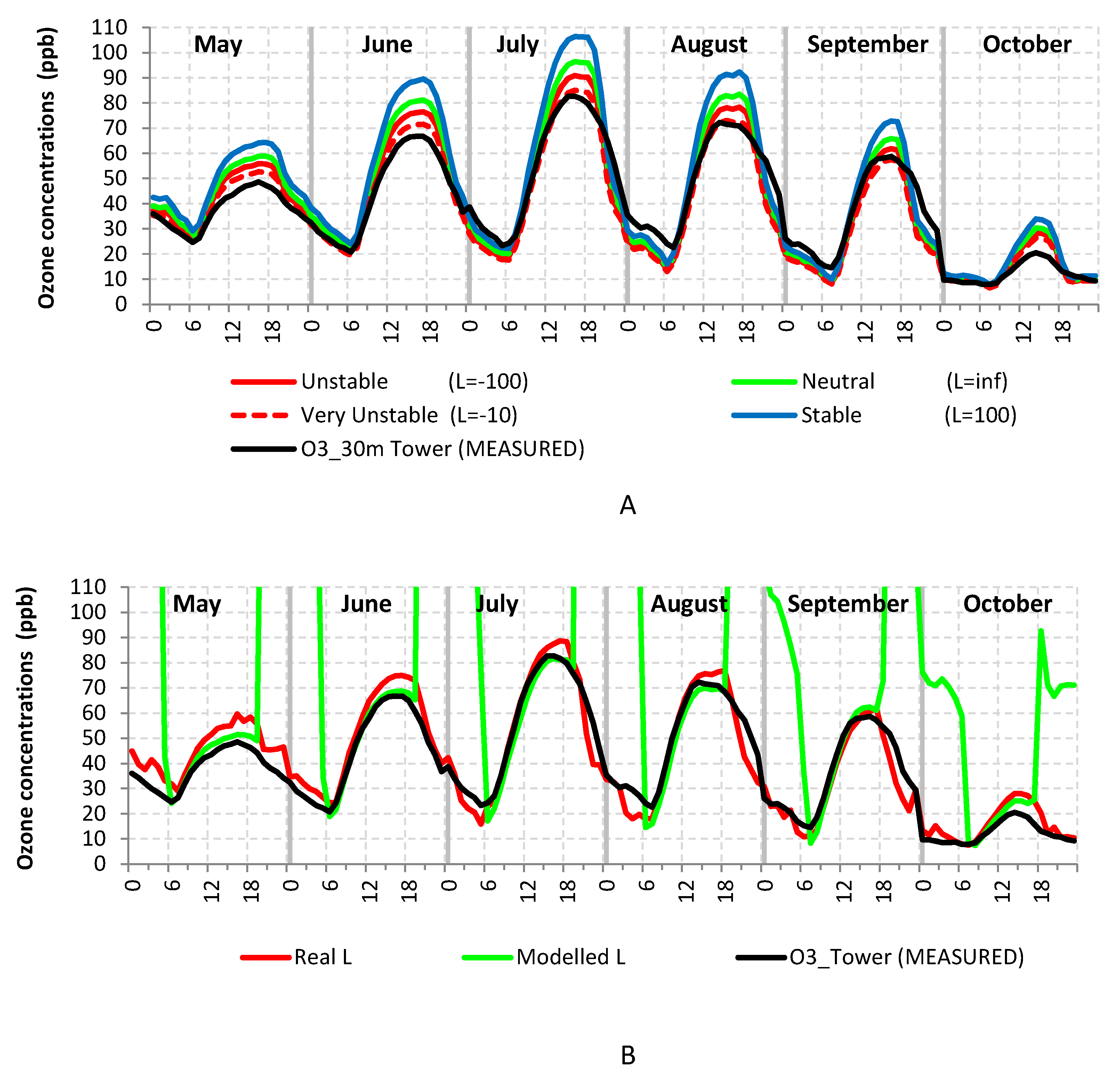
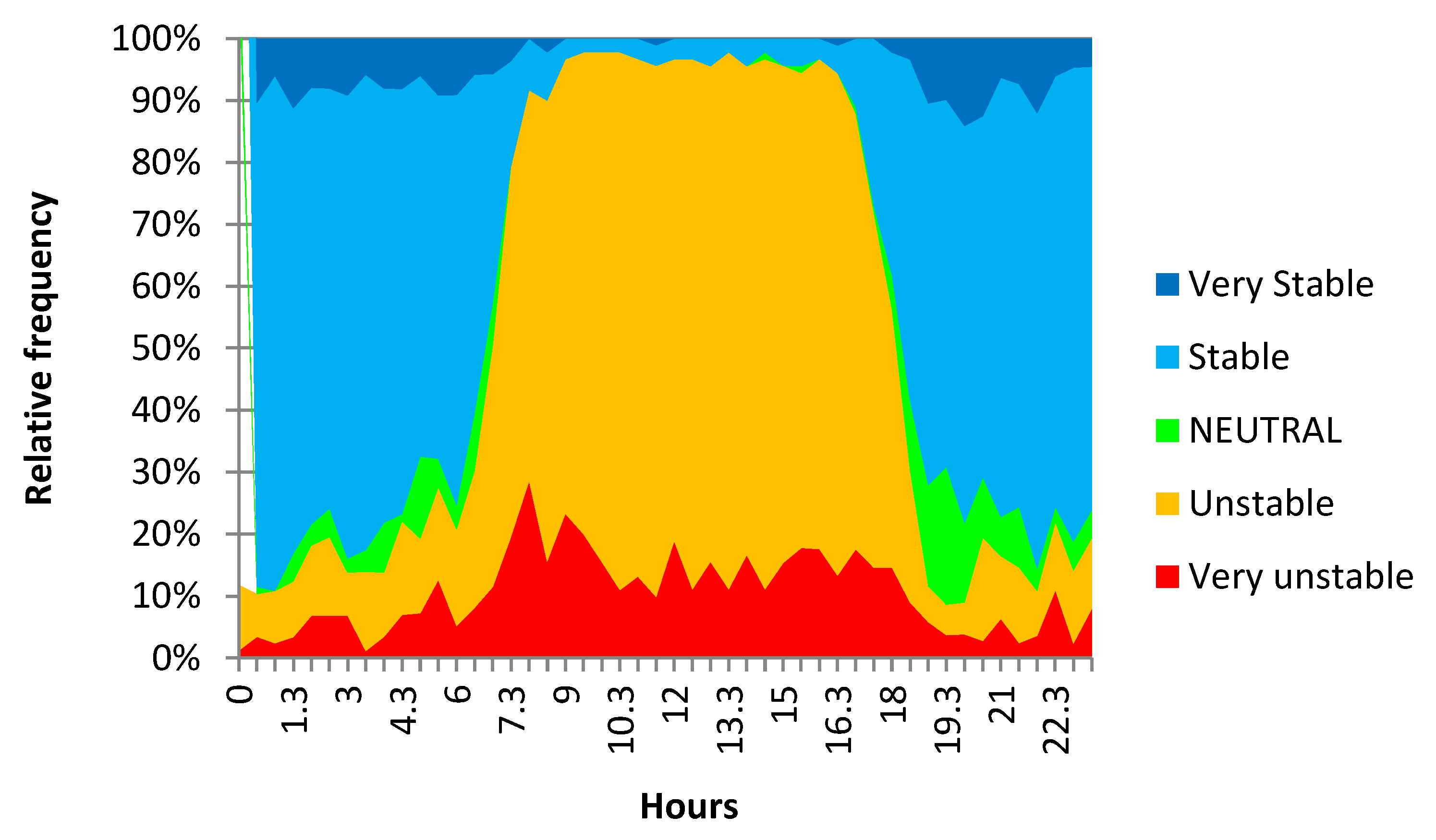
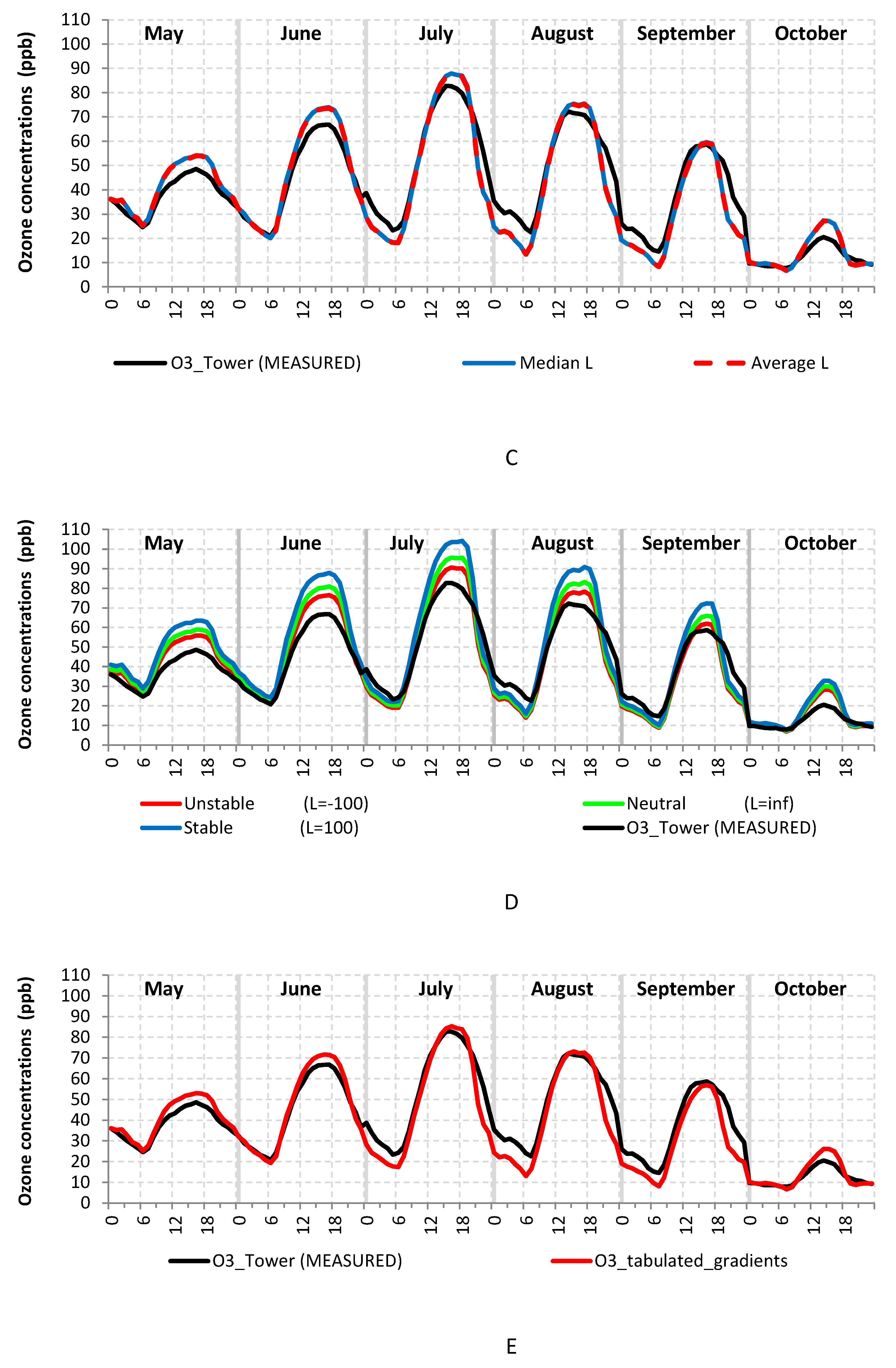
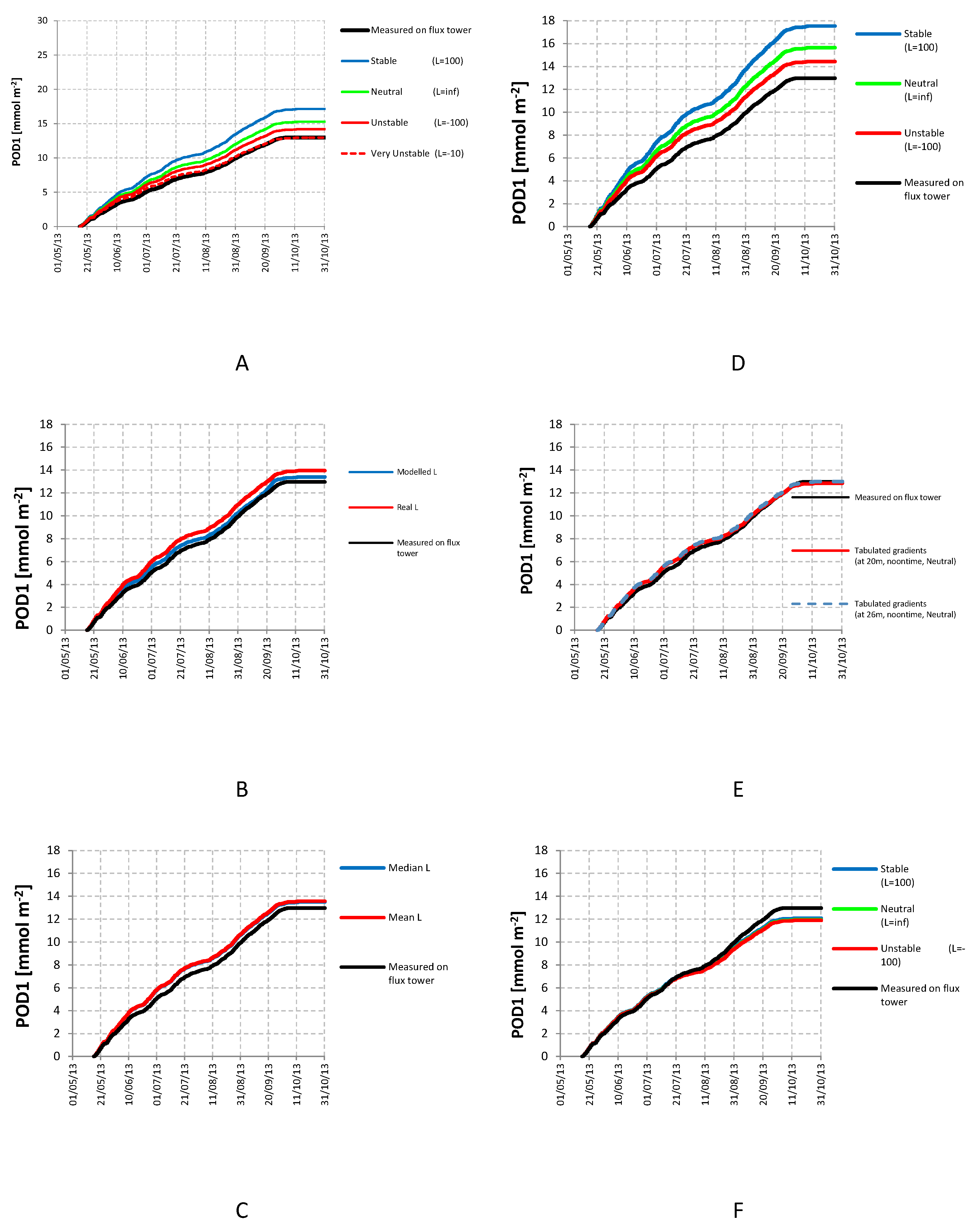
• By using a constant L value representing the different theoretical stability classes of the testing area: 1/L approaching 0 for neutral conditions, 1/L = −0.01 for unstable conditions, 1/L = −0.1 for very unstable conditions, 1/L = +0.01 for stable conditions.
• By using the hourly value of the M-O length L which was obtained:

  (a)

  directly from the eddy covariance measurements;

  (b)

  Bestimation from standard meteorological measurements following the procedure illustrated in Appendix A.

• By using the seasonal average and the median values of the in situ measured M-O length L.
• By using only Equation (1) to calculate the O₃ concentration above the forest top-canopy (by setting z_up = 30 m), i.e., by assuming that the O₃ gradient above the forest was the same as the one calculated above the grassland, thus neglecting the effect of forest geometry and physiology on the O₃ deposition flux.
• By using the noon concentration gradients tabulated in the UN/ECE Mapping Manual [16] suggested for case studies without available meteorological measurements to estimate the value of the M-O length L.
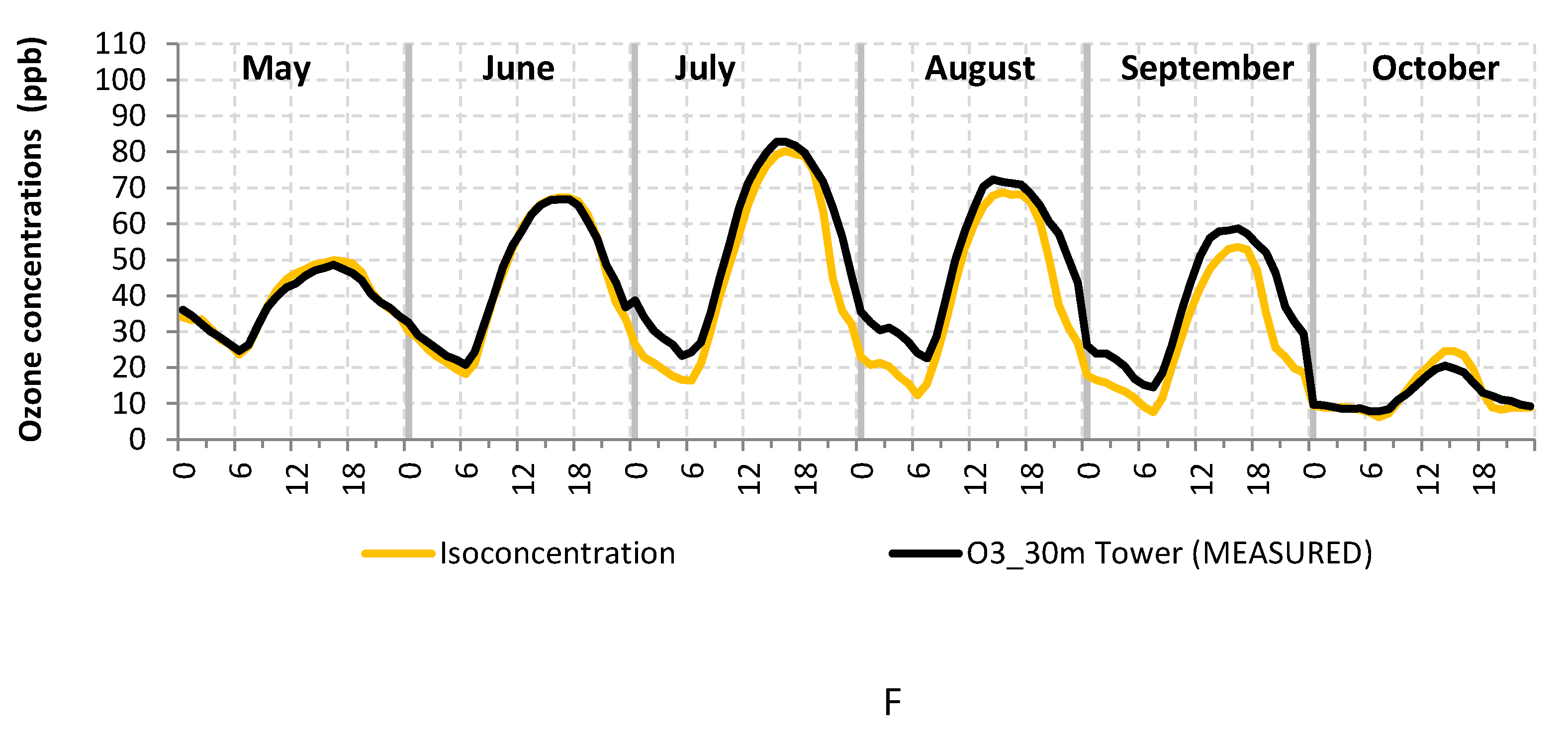
• By directly using the O₃ concentration measured at 2 m above the grassland as a surrogate of the O₃ concentration above the forest top-canopy (no gradients calculation), i.e., by assuming a vertical isoconcentration profile.

Then, the estimated 30 m O₃ concentrations were used to calculate the POD₁ of the forest trees by means of this calculation scheme, and the results were compared with the POD₁ values obtained with the O₃ concentrations measured on the micrometeorological tower according to the procedure illustrated in the previous section.

3. Results

Figure 4 shows the results of the estimations of the O₃ concentration at 30 m a.g.l. above the forest with the different calculation options. When the theoretical stability classes are used (option 1), the estimate that best matched the measured O₃ concentration during the daylight hours was that calculated assuming very unstable conditions (Figure 4A), particularly in the mid-summer months. In the same months, the best match during nighttime was reached when stable conditions were assumed. These results are not surprising observing that the unstable conditions are particularly frequent during daytime while the stable conditions dominate during nighttime (Figure 3). The neutral stability condition, currently assumed in the Mapping Manual [16], implies an overestimation of the ozone concentration by 15% as a median value on a 24-h basis (

Table 2. Differences between the calculated and the measured ozone concentrations above the forest using the different calculation options (see text). For comparison purpose: the Neutral case of option 1 is the output of the current version of the DO3SE model.

Calculation options			Max difference with the O3 measured	Median difference with the O3 measured
1—Theoretical stability	Stable	(L = 100 m)	33%	26%
	Neutral	(L→∞ m)	20%	15%
	Unstable	(L = −100 m)	1%	9%
	Very Unstable	(L = −10 m)	10%	2%
2—Actual stability(*)	Real stability	(measured L)	12%	7%
	Modelled stability	(estimated L)	7%	0%
3—Aver. actual stability	Mean stability	(L = 28.2 m)	12%	5%
	Median stability	(L = 32.4 m)	12%	5%
4—Gradients on ref. veg.	Stable	(L = 100 m)	34%	16%
	Neutral	(L→∞ m)	22%	10%
	Unstable	(L = −100 m)	18%	6%
5—Tab. gradients at 26 m			9%	2%
6—Isoconcentration	Stable	(L = 100 m)	−11%	−4%
	Neutral	(L→∞ m)	−11%	−4%
	Unstable	(L = −100 m)	−11%	−4%

* statistic only restricted to daylight hours.

).

The use of the actual stability (option 2), both derived from the EC measurements or obtained from standard meteorological measurements (modelled L), resulted in better daylight agreement between the estimates and the measurements (Figure 4B). However, during the evening and nighttime, the concentrations estimated with the modelled L are unrealistically high and should be discarded. This happens because the sensible heat flux H estimated with the methodology reported in Appendix A turns rapidly to negative when the solar radiation fades, and this affects the sign of the stability indicator L (Equation (7)) which turns to stable atmosphere. Moreover, when the sunlight fades, the turbulence fades as well, leading to lower values of the friction velocity. The combined effect leads to low positive values of L which indicates an unrealistically extremely stable and stratified atmosphere, where O₃ concentrations increase rapidly with the height.

Nevertheless, since stomata are closed during the night, nighttime O₃ concentrations are of little importance (negligible) for the POD1 accumulation. If we restrict the statistics to the daylight hours (as reported in Table 2), O₃ concentrations estimated when L was modelled show a very good agreement with the measured ones (−0.2% as median difference), while when L was taken from the measurements a median overestimation of 7% was obtained.

The use of the seasonal average of the measured L values (option 3), both as median and mean values, resulted in a better agreement between the estimated and the measured O₃ concentrations than using the actual hourly L values from the measurements (option 2): a 5% overestimation of the median 30 m ozone concentration (Table 2), with a maximum median deviation of 12% was obtained in June (Figure 4C).

When the O₃ gradients were calculated only above the reference surface (option 4), the above canopy O₃ concentrations were overestimated by 6% to 16% according to the different stability classes (Table 2), with the maximum deviation in the central hours of the day, ranging between 18% and 34% (Figure 4D).

The adoption of the noon concentration gradients tabulated in the Mapping Manual (option 5) [16] yielded a good agreement between the estimated and the measured O₃ concentrations, with a median deviation of 2% (Table 2) and a maximum deviation of 9% in the central hours of the day in June (Figure 4E).

Finally, when no gradient calculations were made at all and a vertical O₃ isoconcentration was assumed (option 6), the ground base O₃ concentration measured above the grassland underestimated the top forest O₃ concentration by a median value of −4% (Table 2), and by a maximum deviation of −11% in the central hours of the day (Figure 4F).

The consequences of the different options for the estimation of the top-canopy O₃ concentrations on the POD₁ calculated for a top-canopy leaf are described in Figure 5.

When the theoretical stability classes are used (option 1), the best match between the POD₁ estimated by this calculation procedure and the one obtained from the EC measurements was obtained assuming very unstable atmospheric conditions, which were by far the most frequent conditions at the testing site during the hours when stomata were open (Figure 5A). At the end of the summer semester, the POD₁ calculated with neutral stability conditions perfectly matched the one derived from EC: 12.965 vs. 12.975 mmol O₃ m⁻². When neutral stability conditions are assumed, as in the Mapping Manual [16], the POD₁ at the end of the season overestimated by 18% the one obtained from the EC measurements (

Table 3. Differences between the POD₁ obtained from the EC measurements and the POD₁ calculated with the different calculation options (see text). For comparison purpose: the Neutral case of option 1 is the output of the current version of the DO3SE model.

Calculation options			Diff. with the measured top-canopy POD1
1—Theoretical stability	Stable	(L = 100 m)	+32%
	Neutral	(L→∞ m)	+18%
	Unstable	(L = −100 m)	+9%
	Very Unstable	(L = −10 m)	0%
2—Actual stability	Real stability	(measured L)	+8%
	Modelled stability	(estimated L)	+3%
3—Aver. actual stability	Mean stability	(L = 28.2 m)	+4%
	Median stability	(L = 32.4 m)	+5%
4—Gradients on ref. veg	Stable	(L = 100 m)	+35%
	Neutral	(L→∞ m)	+21%
	Unstable	(L = −100 m)	+11%
5—Tab. gradients at 26radients above crops whenm			0%
6—Isoconcentration	Stable	(L = 100 m)	−7%
	Neutral	(L→∞ m)	−8%
	Unstable	(L = −100 m)	−8%

).

Even when the actual hourly stability values were used (option 2), both taken from the measurements or modelled, the POD₁ estimations were satisfactory, and only slight overestimations between 3% and 8% were obtained (Table 3). Similar results with overestimations between 4% and 5% were obtained when a unique seasonally averaged value of the stability indicator L was used (option 3).

The worst results were obtained when the top-forest ozone concentrations were assumed to be identical to those calculated above the reference surface at the same height of the forest (Figure 5D). With this option (option 4), a POD₁ overestimation of 21% was obtained in neutral conditions.

On the contrary, the POD₁ calculated with the O₃ concentrations obtained from the tabulated gradients of the Mapping Manual (option 5) was in perfect agreement with the one obtained from the EC measurements (Table 3): 13.003 vs. 19.972 mmol O₃ m⁻².

Finally, a −7% to −8% underestimation of the POD₁ was obtained when no vertical gradient corrections were made on the O₃ concentration measured at 2 m above the grassland field nearby.

4. Discussion

The results show that the best estimations of the forest-top ozone concentrations and of the consequent Phytotoxic Ozone Dose POD₁ are obtained when the typical instability conditions of the test site are considered, and even when the tabulated vertical gradient of the Mapping Manual is used.

The latter methodology was obtained from multiple runs of the EMEP deposition module with the meteorology of about 30 sites across Europe, and represents the average conditions at noon above a fully developed crop/forest. Being the atmosphere typically unstable at noon during the summer, it is not surprising that the POD₁ estimated with this methodology fits very well with the measured one. This methodology is the easiest to use compared to the other, and the approach is the most pragmatic one, but we envisage that these results could not be confirmed in all environmental conditions.

On the contrary, the methodologies that require the calculation of the actual hourly L (option 2 with the modeled L, and option 3 with both average and median values of the measured L) are the most scientifically sound but also the most laborious ones. However, the calculation efforts do not always lead to the optimal performances.

The methodology which employs a unique value of L (option 1) allows us to significantly reduce the calculation efforts required to adapt the results to the typical stability conditions of the site. However, optimal performances are reached only when a suitable value of L corresponding to the typical stability conditions is chosen (L = −10 in our testing case), otherwise a general overestimation is expected.

Regardless of the attempt to include the effects of the atmospheric stability, the methodologies that try to excessively simplify the gradient calculation—both completely neglecting the presence of the forest (option 4) or the presence of a vertical ozone gradient (option 6)—lead to significant estimation biases, both as overestimation (option 4) or underestimation (option 6).

In any case, it is worth noting that, in the neutral conditions implicitly assumed by the Mapping Manual methodology for gradient calculations, the POD₁ estimations are generally overestimated.

Since the ozone analyzers and the sampling systems employed to detect the ozone concentrations have accuracies of 1 ppb and precisions between 1 and 2 ppb, any bias in the O₃ measurements can also have an effect on the POD1 estimation. For the four best calculation options (option 1 with unstable conditions, option 2 with modeled L, option 3 with mean measured L, option 5), the introduction of biases of −2 ppb and +2 ppb in the O₃ concentrations resulted in changes between −6% and +7% of the POD₁ estimated with the respective options (

Table 4. Sensitivity of POD₁ estimations to inaccuracies in O₃ concentration measurements. The four best performing options and the current methodology in the Mapping Manual are presented.

Calculation options		Agreement with POD1 measured	+1 ppb	+2 ppb	−2 ppb
1—Theoretical stability	Very Unstable (L = −10 m)	0%	3%	7%	−6%
2—Actual stability	Modelled stability (estimated L)	3%	4%	7%	−7%
3—Aver. actual stability	Mean stability (L = 28.2 m)	4%	3%	6%	−7%
5—Tab. Gradients at 26 m		0%	5%	9%	−5%
Current Mapping Manual	Neutral (L→∞ m)	18%	3%	6%	−6%

). The changes are limited to +3.5% on average if a bias of +1 ppb in O₃ concentration is introduced, with a maximum deviation shown in the case of the tabulated gradients.

These changes in POD₁ estimations are not negligible and highlight the need for special attention to the measuring systems in order to get accurate and precise O₃ measurements. Frequent instrument calibrations and checks, as well as filter changes, are thus needed.

5. Conclusions

The calculation of vertical ozone gradients is needed to avoid erroneous POD₁ and exposure estimations.

The introduction of the atmospheric stability in the DO3SE scheme for the POD₁ calculation improves the accuracy of the stomatal dose estimation compared to that which is obtainable with the current version which implies neutral stability conditions. Actually, in the latter case, an overestimation of O₃ concentrations by 15% as a median value on a 24-h basis has been observed. This feature is likely to be valid in all environmental conditions since the methodology is adaptive.

The tabulated gradients methodology described in the UN/ECE Mapping Manual seems to combine simplicity with good estimation performance on a whole-season time frame, but we fear that this result could not be confirmed in all the different environmental conditions.

Tests on other suitable datasets where eddy covariance flux measurements are available are recommended.

Methodologies that try to excessively simplify the calculation of ozone vertical gradients or that completely neglect the presence of a vertical ozone gradient lead to significant estimation biases.

Inaccuracies in instrumental measurements also have a significant effect on the final POD₁ estimation for forests.

References

1. Paoletti, E.; de Marco, A.; Beddows, D.C.; Harrison, R.M.; Manning, W.J. Ozone levels in European and USA cities are increasing more than at rural sites, while peak values are decreasing. Environ. Pollut. 2014, 192, 295–299. [Google Scholar] [CrossRef] [PubMed]
2. Büker, P.; Feng, Z.; Uddling, J.; Briolat, A.; Alonso, R.; Braun, S.; Elvira, S.; Gerosa, G.; Karlsson, P.E.; Le Thiec, D.; et al. New flux based dose–response relationships for ozone for European forest tree species. Environ. Pollut. 2015, 206, 163–174. [Google Scholar] [CrossRef] [PubMed]
3. Marzuoli, R.; Monga, R.; Finco, A.; Gerosa, G. Biomass and physiological responses of Quercus robur (L.) young trees during 2 years of treatments with different levels of ozone and nitrogen wet deposition. Trees 2016, 30, 1995–2010. [Google Scholar] [CrossRef]
4. Sicard, P.; de Marco, A.; Dalstein-Richier, L.; Tagliaferro, F.; Renou, C.; Paoletti, E. An epidemiological assessment of stomatal ozone flux-based critical levels for visible ozone injury in Southern European forests. Sci. Total Environ. 2016, 541, 729–741. [Google Scholar] [CrossRef] [PubMed]
5. Ochoa-Hueso, R.; Munzi, S.; Alonso, R.; Arroniz-Crespo, M.; Avila, A.; Bermejo, V.; Bobbink, R.; Branquinho, C.; Concostrina-Zubiri, L.; Cruz, C.; et al. Ecological impacts of atmospheric pollution and interactions with climate change in terrestrial ecosystems of the Mediterranean Basin: Current research and future directions. Environ. Pollut. 2017, 227, 194–206. [Google Scholar] [CrossRef] [PubMed]
6. Makar, P.A.; Staebler, R.M.; Akingunola, A.; Zhang, J.; McLinden, C.; Kharol, S.K.; Pabla, B.; Cheung, P.; Zheng, Q. The effects of forest canopy shading and turbulence on boundary layer ozone. Nat. Commun. 2017, 8. [Google Scholar] [CrossRef] [PubMed]
7. Wesely, M.L.; Hicks, B.B. Some factors that affect the deposition rates of sulfur dioxide and similar gases on vegetation. J. Air Pollut. Control Assoc. 1977, 27, 1110–1116. [Google Scholar] [CrossRef]
8. Wolfe, G.M.; Thornton, J.A.; McKay, M.; Goldstein, A.H. Forest-atmosphere exchange of ozone: Sensitivity to very reactive biogenic VOC emissions and implications for in-canopy photochemistry. Atmos. Chem. Phys. 2011, 11, 7875–7891. [Google Scholar] [CrossRef] [Green Version]
9. De Arellano, J.V.G.; Duynkerke, P.G. Influence of chemistry on the flux-gradient relationships for the NO-O3-NO2 system. Bound.-Layer Meteorol. 1992, 61, 375–387. [Google Scholar] [CrossRef]
10. Tuovinen, J.P.; Simpson, D. An aerodynamic correction for the European ozone risk assessment methodology. Atmos. Environ. 2008, 42, 8371–8381. [Google Scholar]
11. Grünhage, L.; Haenel, H.D.; Jäger, H.J. The exchange of ozone between vegetation and atmosphere: Micrometeorological measurement techniques and models. Environ. Pollut. 2000, 109, 373–392. [Google Scholar] [CrossRef]
12. Finnigan, J. Turbulence in plant canopies. Annu. Rev. Fluid Mech. 2000, 32, 519–571. [Google Scholar] [CrossRef]
13. Katul, G.; Cava, D.; Poggi, D.; Albertson, J.; Mahrt, L. Stationarity, Homogeneity, and Ergodicity in Canopy Turbulence. In Handbook of Micrometeorology; Lee, X., Massman, W., Law, B., Eds.; Springer: Dordrecht, The Netherlands, 2004; volume 29. [Google Scholar]
14. Tuovinen, J.P.; Emberson, L.; Simpson, D. Modelling ozone fluxes to forests for risk assessment: Status and prospects. Ann. For. Sci. 2009, 66, 1–14. [Google Scholar] [CrossRef]
15. Emberson, L.D.; Ashmore, M.R.; Cambridge, H.M.; Simpson, D.; Tuovinen, J.P. Modelling stomatal ozone flux across Europe. Environ. Pollut. 2000, 109, 403–413. [Google Scholar] [CrossRef]
16. CLRTAP-UNECE Convention on Long-Range Transboundary Air Pollution. Mapping Critical Levels for Vegetation. Chapter III of Manual on Methodologies and Criteria for Modelling and Mapping Critical Loads and Levels and Air Pollution Effects, Risks and Trends. 2015. Available online: http://icpvegetation.ceh.ac.uk/publications/documents/Ch3-MapMan-2016-05-03_vf.pdf (accessed on 15 October 2016).
17. Garratt, J.R. The atmospheric boundary layer. Earth-Sci. Rev. 1994, 37, 89–134. [Google Scholar] [CrossRef]
18. Gerosa, G.; Ballarin-Denti, A. Regional scale risk assessment of ozone and forests. Dev. Environ. Sci. 2003, 3, 119–139. [Google Scholar]
19. Simpson, D.; Benedictow, A.; Berge, H.; Bergström, R.; Emberson, L.D.; Fagerli, H.; Flechard, C.R.; Hayman, G.D.; Gauss, M.; Jonson, J.E.; et al. The EMEP MSC-W chemical transport model–technical description. Atmos. Chem. Phys. 2012, 12, 7825–7865. [Google Scholar] [CrossRef] [Green Version]
20. Van Pul, W.A.J.; Jacobs, A.F.G. The conductance of a maize crop and the underlying soil to ozone under various environmental conditions. Bound.-Layer Meteorol. 1994, 69, 83–99. [Google Scholar] [CrossRef]
21. Monin, A.S.; Obukhov, A.M. Osnovnye zakonomernosti turbulentnogo peremesivanija v prizemnom sloe atmosfery (Basic laws of turbulent mixing in the atmosphere near the ground). Trudy geofiz. Inst. AN SSSR 1954, 24, 163–187. [Google Scholar]
22. Gerosa, G.; Finco, A.; Marzuoli, R.; Tuovinen, J.P. Evaluation of the uncertainty in the ozone flux effect modelling: From the experiments to the dose–response relationships. Atmos. Environ. 2012, 54, 44–52. [Google Scholar] [CrossRef]
23. Jarvis, P.G. The interpretation of the variations in leaf water potential and stomatal conductance found in canopies in the field. Philos. Trans. R. Soc. Lond. Ser. B: Biol. Sci. 1976, 273, 593–610. [Google Scholar] [CrossRef]
24. Büker, P.; Morrissey, T.; Briolat, A.; Falk, R.; Simpson, D.; Tuovinen, J.P.; Alonso, R.; Barth, S.; Baumgarten, M.; Grulke, N.; et al. DO3SE modelling of soil moisture to determine ozone flux to European forest trees. Atmos. Chem. Phys. Discuss. 2011, 11, 33583–33650. [Google Scholar] [CrossRef] [Green Version]
25. Longo, L. Rapporti Scientifici 1. Centro Nazionale Biodiversità Forestale Verona-Bosco della Fontana. In Dinamica di una foresta della Pianura Padana. Bosco della Fontana. Seconda edizione con Linee di gestione forestale; Mason, F., Ed.; Gianluigi Arcari Editore: Mantua, Italy, 2006; pp. 16–17. [Google Scholar]
26. Güsten, H.; Heinrich, G.; Schmidt, R.W.H.; Schurath, U. A novel ozone sensor for direct eddy flux measurements. J. Atmos. Chem. 1992, 14, 73–84. [Google Scholar]
27. Güsten, H.; Heinrich, G. On-line measurements of ozone surface fluxes: Part I. Methodology and instrumentation. Atmos. Environ. 1996, 6, 897–909. [Google Scholar] [CrossRef]
28. Vickers, D.; Mahrt, L. Quality Control and Flux Sampling Problems for Tower and Aircraft Data. J. Atmos. Ocean. Technol. 1997, 14, 512–526. [Google Scholar] [CrossRef]
29. Lee, X.; Massman, W.; Law, B. Handbook of Micrometeorology: A Guide for Surface Flux Measurements and Analysis; Springer: Dordrecht, The Netherlands, 2004. [Google Scholar]
30. Aubinet, M.; Vesala, T.; Papale, D. Eddy Covariance: A Practical Guide to Measurement and Data Analysis; Springer: Dordrecht, The Netherlands, 2012; p. 438. [Google Scholar]
31. Rummel, U.; Ammann, C.; Kirkman, G.A.; Moura, M.A.L.; Foken, T.; Andreae, M.O.; Meixner, F.X. Seasonal variation of ozone deposition to a tropical rain forest in southwest Amazonia. Atmos. Chem. Phys. 2007, 7, 5415–5435. [Google Scholar] [CrossRef]
32. Muller, J.B.A.; Percival, C.J.; Gallagher, M.W.; Fowler, D.; Coyle, M.; Nemitz, E. Sources of uncertainty in eddy covariance ozone flux measurements made by dry chemiluminescence fast response analysers. Atmos. Meas. Tech. 2010, 3, 163–176. [Google Scholar] [CrossRef]
33. Webb, E.K.; Pearman, G.I.; Leuning, R. Correction of flux measurements for density effects due to heat and water vapour transfer. Q. J. R. Meteorol. Soc. 1980, 106, 85–100. [Google Scholar] [CrossRef]
34. Foken, T.; Wichura, B. Tools for quality assessment of surface-based flux measurements. Agric. For. Meteorol. 1996, 78, 83–105. [Google Scholar] [CrossRef]
35. Gerosa, G.; Vitale, M.; Finco, A.; Manes, F.; Ballarin-Denti, A.; Cieslik, S. Ozone uptake by an evergreen Mediterranean forest (Quercus ilex) in Italy. Part I: Micrometeorological flux measurements and flux partitioning. Atmos. Environ. 2005, 39, 3255–3266. [Google Scholar] [CrossRef]
36. Gerosa, G.; Cieslik, S.; Ballarin-Denti, A. Micrometeorological determination of time-integrated stomatal ozone fluxes over wheat: A case study in Northern Italy. Atmos. Environ. 2003, 37, 777–788. [Google Scholar] [CrossRef]
37. Holtslag, A.A.; van Ulden, A.P. A simple scheme for daytime estimates of the surface fluxes from routine weather data. J. Appl. Meteorol. Climatol. 1983, 22, 517–529. [Google Scholar] [CrossRef]
38. NOAA, US Department of Commerce: National Oceanic and Atmospheric Administration. Solar Calculation Details. Available online: http://www.esrl.noaa.gov/gmd/grad/solcalc/calcdetails.html (accessed on 15 October 2016).
39. Beljaars, A.C.M.; Holtslag, A.A. A software library for the calculation of surface fluxes over land and sea. Environ. Softw. 1989, 5, 60–68. [Google Scholar] [CrossRef]
40. Beljaars, A.C.M.; Holtslag, A.A. Flux parametrization over land surfaces for atmospheric models. J. Appl. Meteorol. 1991, 30, 327–341. [Google Scholar] [CrossRef]
41. Hanna, S.R.; Chang, J.C. Boundary layer parametrizations for applied dispersion modeling over urban areas. Bound.-Layer Meteorol. 1992, 58, 229–259. [Google Scholar] [CrossRef]
42. Doll, D.; Ching, J.K.S.; Kaneshire, J. Parametrization of subsurfaces heating for soil and concrete using new radiation data. Bound.-Layer Meteorol. 1985, 32, 351–372. [Google Scholar] [CrossRef]
43. Bassin, S.; Calanca, P.; Weidinger, T.; Gerosa, G.; Fuhrer, J. Modeling seasonal ozone fluxes to grassland and wheat: Model improvement, testing and application. Atmos. Environ. 2003, 38, 2349–2359. [Google Scholar] [CrossRef]
44. WMO (World Meteorological Organization). Guide to Meteorological Instruments and Methods of Observation, 7th Edition ed. 2008. Available online: https://www.wmo.int/pages/prog/gcos/documents/gruanmanuals/CIMO/CIMO_Guide-7th_Edition-2008.pdf (accessed on 15 October 2016).
Figure 1. Ozone gradients with different atmospheric stability conditions (neutral, stable, unstable). A Gradients above crops when O3 is measured above the canopy top. B gradients above a forest (target surface) when O3 concentration is measured above a reference surface with lower vegetation near to the forest edge at a height which is lower than the forest top-canopy height. Thick curves are the O3 gradients above the reference surface generated from the measuring point (yellow/red dot); dashed curves are the O3 gradients above the forest canopy.
Forests 08 00337 g001
Figure 2. Resistive network for the calculation of the O3 concentration at the top of a target canopy (e.g., forest) when ozone and meteorological measurements are available above a different vegetated surface (e.g., grassland). Uppercase resistances refer to the forest while lowercase resistances refer to the grassland. See the text for the meaning of the symbols.
Forests 08 00337 g002
Figure 3. Atmospheric stability conditions between May and July 2013 at the Bosco Fontana forest site.
Forests 08 00337 g003
Figure 4. Average daily course of ozone concentrations estimated at 30 m a.g.l. above the forest in the indicated months by following the different calculation options (see text): A theoretical stability (option 1); B actual stability (options 2A and 2B); C average stability (option 3); D ozone above grassland (option 4); E tabulated gradients (option 5); F isoconcentration (option 6). For comparison purpose: the Neutral case of option 1 (Figure 4A) is the output of the current version of the DO3SE model.
Forests 08 00337 g004aForests 08 00337 g004bForests 08 00337 g004c
Figure 5. Phytotoxic Ozone Dose (POD1) for a top-canopy leaf: comparison of the POD1 obtained from the eddy covariance (EC) measurements and the POD1 calculated with the different calculation options (see text): A theoretical stability (option 1); B actual stability (options 2A and 2B); C average stability (option 3); D ozone above grassland (option 4); E tabulated gradients (option 5); F isoconcentration (option 6). For comparison purpose: the Neutral case of option 1 (Figure 5A) is the output of the current version of the DO3SE model.
Forests 08 00337 g005