Relationship between Soil Characteristics and Stand Structure of Robinia pseudoacacia L. and Pinus tabulaeformis Carr. Mixed Plantations in the Caijiachuan Watershed: An Application of Structural Equation Modeling

Abstract

In order to study the multi-factor coupling relationships between typical Robinia pseudoacacia L. and Pinus tabulaeformis Carr. mixed plantations in the Caijiachuan basin of the Loess Plateau of Shanxi Province, West China, 136 sample plots were selected for building a structural equation model (SEM) of three potential variables: terrain, stand structure, and soil characteristics. Additionally, the indicators (also known as observed variables) were studied in this paper, including slope, altitude, diameter at breast height (DBH), tree height (TH), tree crown area, canopy density, stand density, leaf area index (LAI), soil moisture content, soil maximum water holding capacity (WHC), soil organic matter (SOM), total nitrogen (TN), total phosphorus (TP), ammonia-nitrogen (NH₃-N), nitrate-nitrogen (NO₃-N), and available phosphorus (AP). The results showed that terrain was the most important factor influencing soil moisture and nutrients, with a total impact coefficient of 1.303 and a direct path coefficient of 0.03, which represented mainly positive impacts; while correspondingly stand structure had a smaller negative impact on soil characteristics, with a total impact coefficient of −0.585 and a direct path coefficient of −0.01. The terrain also had a positive impact on the stand structure, with a total impact coefficient of 0.487 and a direct path coefficient of 0.63, indicating that the topography factors were more suitable for site conditions and both the stand structure and the soil moisture and nutrient conditions were relatively superior. By affecting the stand structure, terrain could restrict some soil, water, and nutrient functions of soil and water conservation. The influence coefficients of the four observed variables of DBH, stand density, soil water content, and organic matter, and potential variable topography reached 0.686, −0.119, 1.117, and 0.732, respectively; and the influence coefficients of soil moisture, organic matter and stand structure were −0.502 and −0.329, respectively. Therefore, besides observing the corresponding latent variables, the observed variables had a considerable indirect influence on other related latent variables. These relationships showed that the measures, such as changing micro-topography and adjusting stand density, should effectively maintain or enhance soil moisture and nutrient content so as to achieve improved soil and water conservation benefits in the ecologically important Loess Area.

1. Introduction

Large-scale afforestation in the Western Shanxi Loess Area started in the early 1990s, and the area has been covered by larger-sized plantations over the past 20 years. Mixed afforestation methods—with plantations consisting of two or more tree species—are often used. In the mixed plantations, tree species other than the main tree species represent over 20% of the plantation, in terms of number of trees, cross-sectional area, or volume. The impact of vegetation construction on soil and water resources has also aroused great attention, both at home and abroad, particularly in the Loess Plateau—an area known for soil and water loss, a lack of water resources, a fragile ecological environment, and a lack of a strong conservation ethics. The main reasons for the creation of large-scale plantations in this region, and their impacts on soil and water conservation, water resources security, and regional sustainable development, have been a particular cause for concern. The relationships between the stand structures of the plantations and soil and water conservation have also gradually become the foci of academic research.

Many studies on the stand structure and soil and water conservation functions of the Loess Plateau, as well as other ecologically sensitive areas, have been carried out, usually aimed at one, or several, dimensions. For example, Bi Huaxing et al. utilized the principle of water balance to establish a suitable coverage calculation model based on spatial and temporal differentiation of soil moisture and water consumption [1]; Brzostek et al. proposed that chronic water stress could reduce the tree growth of forests, and also considered the extent to which forests ameliorate climate warming [2]; and Panagos et al. presented an assessment of soil loss due to water erosion in Europe, and also suggested some policy measures that should be targeted [3]. Other scholars have also presented research results on some factors related to the stand structure, soil moisture [4,5], and soil nutrients [6] in the Loess Plateau. However, research on the multi-factor coupling relationships between stand structure and soil moisture and nutrients [7] is relatively lacking. Traditionally, the main functions of water and soil conservation in gully areas of this type are regarded as water resource conservation and erosion reduction [8]. Water conservation has manifested as soil water storage capacity and soil conservation often incorporates the preservation, storage, recycling, conversion, and acquisition of soil organic matter, nitrogen, phosphorus, and other nutrients [9].

Structural equation modeling (SEM) has become increasingly precise and is now widely used in ecological studies [10,11,12,13], mainly for the purpose of quantifying the relationships between multiple factors. Essentially, SEM aims to generate strong and distinct links between theoretical and experimental ideas [14]. The ability to disentangle causal relationships and to test competing models and theories (as opposed to null hypotheses) are key strengths of SEM methods [15]. Due to their statistical strength and applicability, SEM approaches have been employed in a wide range of environmental and ecological studies [16,17,18,19]. For example, SEM has been applied to evaluate the effect of grazing on ecosystem processes [20,21]; the relationships between fire and edaphic factors and woody vegetation structure and composition [22]; the sensitivity of soil respiration to environmental factors [23]; the impacts of land uses on stream integrity [24]; the factors that affect plant richness in recovering forests [25,26]; the relationships associated with the decline in species richness, as natural landscapes undergo conversion to human-dominated landscapes [27]; and both the direct and indirect association of plant species richness to landscape conditions and local environmental factors [28,29]. However, to our knowledge, SEM methods have not been applied to study stand structure impacts on soil and water conservation.

In this paper, the covariance SEM is used to quantify the multi-factor coupling relationship between soil moisture and nutrients in typical plantations. Soil moisture content and soil maximum water holding capacity are taken as water conservation indicators, and organic matter, nitrogen, and phosphorus are used as conservation soil indicators. These indicators are all used to study soil characteristics and their relationships with the topography and stand structure in order to reveal the role of stand structure on the conservation of water sources and soil function mechanisms, and to further provide references of control technology regarding the practical and suitable slope stand structural adjustments in the Loess Plateau.

2. Materials and Methods

2.1. Site Description

The Caijiachuan Watershed served as the study site; it is located on the Loess Plateau in Ji County, Shanxi Province, China (35°53’–36°21’ N, 110°27’–111°7’ E; elevation 904–1592 m), and is a typical gully area. Meteorological records indicate that the long-term mean annual air temperature is 10.2 °C and the frost-free period is 172 days. The average annual precipitation is 571 mm, with an uneven distribution. The average annual potential evapotranspiration (PET) is 1724 mm, which far exceeds the rainfall. Inside this area, the type of soil is mainly Haplic Luvisols (Soil classification of the Food and Agriculture Organization of the United Nations) and is mostly alkaline. There are mainly artificial shelterbelts of black locust (Robinia pseudoacacia L.) and Chinese pine (Pinus tabulaeformis Carr.) in the nested watershed, with an area of 38 km² and a forest cover rate of 72%. The main shrubs under the forests are periploca (Periploca sepium Bunge), yellow rose (Rosa xanthine Lindl.), sophora viciifolia (Sophora davidii (Franch.) Skeels), meadowsweet (Spiraea salicifolia L.), lilac (Syringa linn.), elaeagnus umbellata (Elaeagnus pungens Thunb.), etc. Through the investigation of forestland, shrubland, and grassland in this area, dominant species of artificial R. pseudoacacia and P. tabulaeformis forests with different slopes, aspects, and altitudes were selected as objects and studied.

2.2. Data Acquisition and Processing Methods

Thirty-four standard plots of 20 m × 20 m were set up at the plantations and 136 sample plots of 10 m × 10 m were set up with shady, semi-shady, sunny, and semi-sunny aspects (one standard plot was divided into four equal sample plots to reduce the heterogeneity) The slopes of the plots ranged from 15° to 45°, and were distributed at an average elevation of 1133.5 m above sea level (

Table 1. The distribution of aspects, slopes, and altitudes of the sample plots in the Caijiachuan Watershed.

Aspect	Shady		Semi-Shady	Sunny		Semi-Sunny
Sample quantity	7		11	6		10
Slope/°	≤15		16–25	26–35		≥36
Sample quantity	2		15	15		2
Altitude/m	900–1000	1000–1100	1100–1150	1150–1200	1200–1300	>1300
Sample quantity	2	6	15	8	3	0

Notes: (1) The distribution of aspect tends to be mostly homogeneous. (2) The lands featuring gentle slopes (≤15) are usually cropland and those that are dangerously steep (≥36) are difficult sites to access, as such, there are very few of either type of these sites for afforestation, whereas many sites with deep slopes (16–35) are used for afforestation in order to restore vegetation and improve the environment in China. (3) In the watershed, low-altitude (900–1000 m) areas are mainly agricultural lands or areas where people are living, so there are very few low-altitude sites for afforestation; high-altitude (>1300 m) areas are mainly distributed with natural forests, so there are no high-altitude plantations; the mid-altitude areas (1000–1300 m) are the main afforestation areas of mixed plantations, and can therefore be regarded as being representative of the mixed plantations in the region.

). The mixture of plantation species consisted of R. pseudoacacia and P. tabulaeformis at a ratio of 8:2, as R. pseudoacacia was the dominant species. Using individual field measurements in these plots, the varieties of trees, diameter at breast height (DBH), tree height (TH), and tree crown area were measured, and then the canopy density and stand density were calculated. The leaf area indices of the quadrats were determined using a LAI-2000 (LI-COR Company, ‎Lincoln, NE, USA) vegetation canopy analyzer. According to the trophic classification scheme for functions of soil and water conservation [8], indicators of water resources and soil protection were confirmed. Mixed soil samples, 0–60 cm, were collected using the cutting ring method and were representative of forest soils in this area; soil moisture content was determined using the drying method; and water holding capacity (WHC) was measured using the soil infiltration method [30]. After air-dried soil was sieved (0.15 mm sieve), indoor experiments were conducted. The contents of soil organic matter (SOM), total nitrogen (TN), total phosphorus (TP), ammonia-nitrogen (NH₃-N), nitrate-nitrogen (NO₃-N), and available phosphorus (AP) were measured with a SmartChem-200 (AMS/Alliance Instruments, Paris, France) discrete wet chemistry analyzer. The major geographical and biological characteristics of the investigated plots are summarized in

Table 2. The survey of the species of Robinia pseudoacacia L. and Pinus tabulaeformis Carr. mixed plantations in the Caijiachuan Watershed, Shanxi Province, West China. DBH, diameter at breast height; LAI, leaf area index; WHC, water holding capacity; SOM, soil organic matter; TN, total nitrogen; TP, total phosphorus; NH3-N, ammonia-nitrogen; NO3-N, nitrate-nitrogen; AP, available phosphorus.

Stands and Soil Characteristics	Maximum	Minimum	Average
Slope (°)	45	15	26.50
Altitude (m)	1220	960	1133.53
DBH (cm)	18.54	6.37	10.85
Tree height (m)	13.4	3.0	8.2
Crown area (m2)	16.74	2.80	8.12
Canopy density	0.88	0.38	0.64
Stand density (trees∙hectare−1)	4400	500	1679
LAI	4.50	0.88	2.06
Soil moisture content (%)	40.03	5.66	13.71
WHC (%)	122.88	25.54	50.41
SOM (g∙kg−1)	122.55	1.31	16.08
TN (g∙kg−1)	4.65	0.01	0.69
TP (g∙kg−1)	7.60	0.03	0.66
NH3-N (mg∙kg−1)	66.84	2.79	20.99
NO3-N (mg∙kg−1)	88.40	0.12	10.27
AP (mg∙kg−1)	117.64	0.16	36.00

.

2.3. Structural Equation Modeling

SEMs (also known as path analyses) are statistical multivariate models that are used to estimate causality and direct or indirect relationships between multiple variables [31]. These models are less restrictive than regression models in that some variables may play the role of predictor variable and dependent variable simultaneously [32,33]. SEM starts by constructing an a priori schema: an analytical model that represents all hypothetical causal links between the predictors and the response variables, based on previous knowledge of the ecological system [34].

Thus, SEM in ecology is a method to test ecosystem structure and function [35], which is closely related to (and is actually a more general form of) several types of statistical analyses, including regression, principal components analysis (PCA), and path analysis [36]. Furthermore, it can explore the relationships between observed variables, latent variables, and residuals to quantitatively describe the influence of independent variables on dependent variables, including direct, indirect, and total impacts [13]. However, in contrast to some other methods, SEM provides a means to evaluate both the structure of the model as well as a specific parameterization of the model structure using data [37]. By “model structure”, we mean the pattern of relationships among variables (correlations, direct, and indirect relationships among variables). The structural equation model includes two parts of the measurement model and the structural model; the formula is as follows [38,39,40]:

$$X=\Lambda x\xi +\delta$$

(1)

$$Y=\Lambda y\eta +\epsilon$$

(2)

$$\eta ={\rm B}\eta +\Gamma \xi +\zeta$$

(3)

Equations (1) and (2) are measurement models, used to describe the relationship between latent and observed variables, where X is the exogenous observation variable vector, Y is the endogenous observation variable vector, $\Lambda x$ and $\Lambda y$ are the factor loadings of the indicator variables (X, Y), $\delta$ and $\epsilon$ are the measurements of the exogenous observation variables and the endogenous observation variables, $\xi$ is the exogenous latent variable, and $\eta$ is the endogenous latent variable.

Equation (3) is a structural model that can reflect the relationships between the potential variables, where ${\rm B}$ is the structural coefficient matrix of the relationship between endogenous latent variables, $\Gamma$ is the structural coefficient matrix of the relationships between endogenous latent variables and exogenous latent variables, and $\zeta$ is the interference factor or residual value of the structural model. The initial model with the aid of a path map reflects the relationships among the variables in the structural model, and the path coefficients represent the extent of the relationship between the variables. After the path diagram is established, the path coefficients of all the paths are usually calculated using the maximum likelihood method [13], which is also used in this study.

The climate, hydrology, and other environmental conditions in the area were basically the same, and the different topographical factors (${\xi }_1$) were used as potential exogenous variables. The slope, aspect, slope position, and altitude were taken into account in the modeling. In consideration of the aspect and slope position being subject to qualitative description and random selection in the survey, the slope ($x_1$) and elevation ($x_2$) were determined to be the index of the initial model belonging to the exogenous observation variables, because they are the indicators of accurate measurement. Their corresponding errors are ${\delta }_1$ and ${\delta }_2$, respectively.

The differences between quadrats were also reflected in the stand structure (${\xi }_2$). The measuring indices affecting the stand structure mainly included DBH ($x_3$), TH ($x_4$), tree crown area ($x_5$), canopy density ($x_6$), stand density ($x_7$), and LAI ($x_8$), which were also exogenous observation variables as well. The corresponding errors were ${\delta }_3,{\delta }_4,{\delta }_5,{\delta }_6,{\delta }_7,$ and ${\delta }_8$. Soil properties ($\eta$) were taken as potential endogenous variables, and their corresponding indices, such as soil moisture content ($y_1$), WHC ($y_2$), SOM ($y_3$), TN ($y_4$), TP ($y_5$), NH₃-N ($y_6$), NO₃-N ($y_7$), and AP ($y_8$), were determined as endogenous observation variables, of which the corresponding errors were ${\epsilon }_1$, ${\epsilon }_2$, ${\epsilon }_3$, ${\epsilon }_4$, ${\epsilon }_5$, ${\epsilon }_6$, ${\epsilon }_7,$ and ${\epsilon }_8$. In addition, the modeling process needed to consider the residuals of three potential variables as ${\zeta }_1$, ${\zeta }_2,$ and ${\zeta }_3$.

After creating an initial model based on previous knowledge, site information, and background data, a chi-square value (${\chi }^2$) test was then conducted to examine whether the covariance structure suggested by the model satisfactorily fits the covariance structures [19]. The ${\chi }^2$, degree of freedom ($df$, 0 ≤ ${\chi }^2$/$df$ ≤ 3), probability level (p > 0.05), root mean square error of approximation (0 ≤ root meant square error of approximation (RMSEA) ≤ 0.05) [40], and comparative fit index (0.9 ≤ comparative fit index (CFI) ≤ 1.00) were given to determine the “best” model that has the highest predictive performance, while the comparative fit index (0.7 ≤ CFI ≤ 0.90) was “tolerable” [41]. If the parameters exhibit beyond the proper range after model running the model, we should use two methods for model correction: “modification index” and “critical ratio (CR) for difference”, provided by the Amos 22.0 software (IBM/International Business Machines Corporation, Armonk, NY, USA) package. In the model diagram, the double arrow (“<->“) section was the covariance correction index between the residual variables, and the single arrow (“-->“) section was a regression weight correction index between variables, indicating that if an arrow is added between two variables, at least the chi-squared value of the model will be reduced. In addition, the CR statistic followed a normal distribution, so its value can be used to judge whether there is a significant difference between the two estimated parameters. In this study, the former method was selected to modify the model, according to the characteristics of the investigated measurable variables.

3. Results

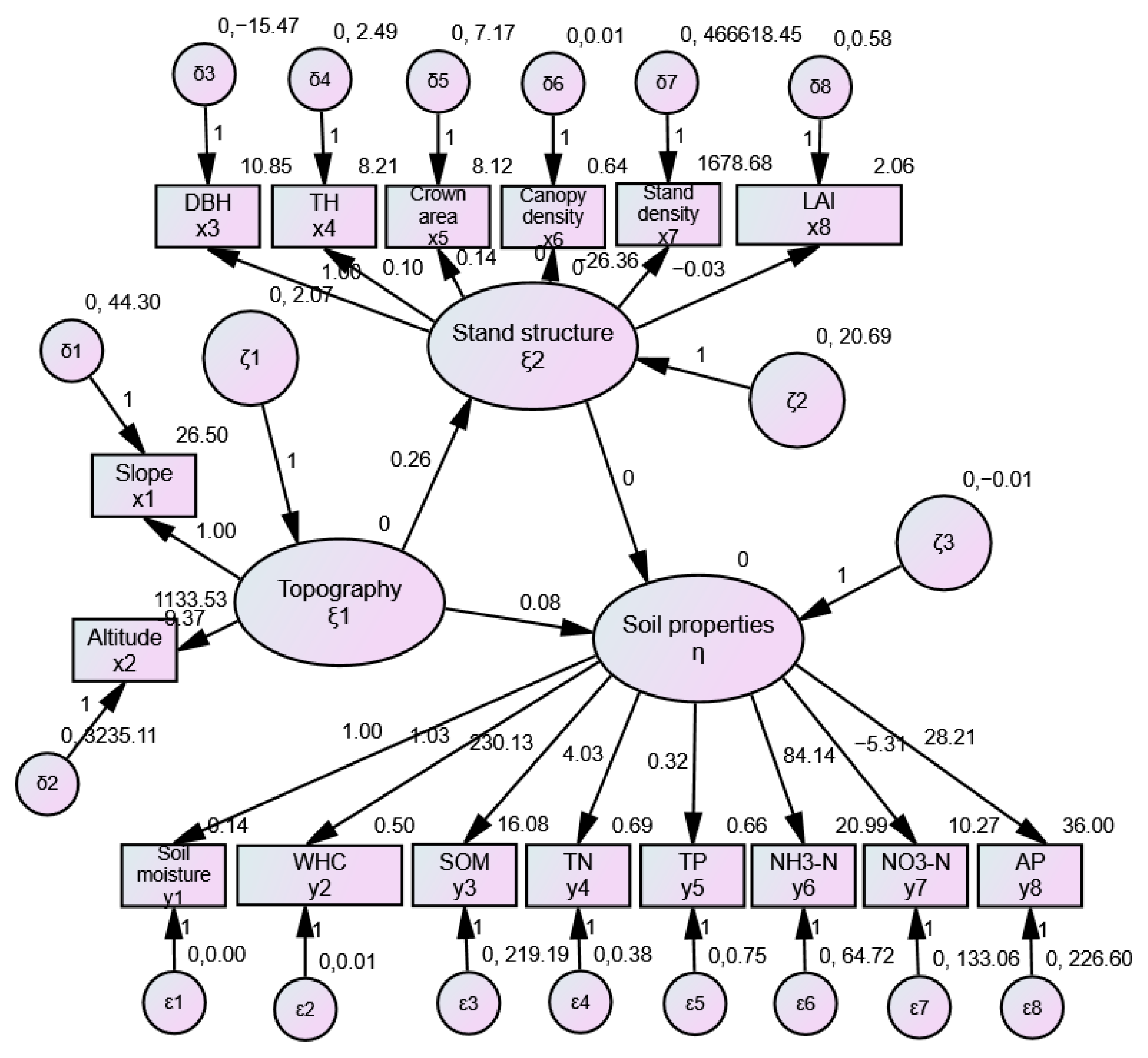
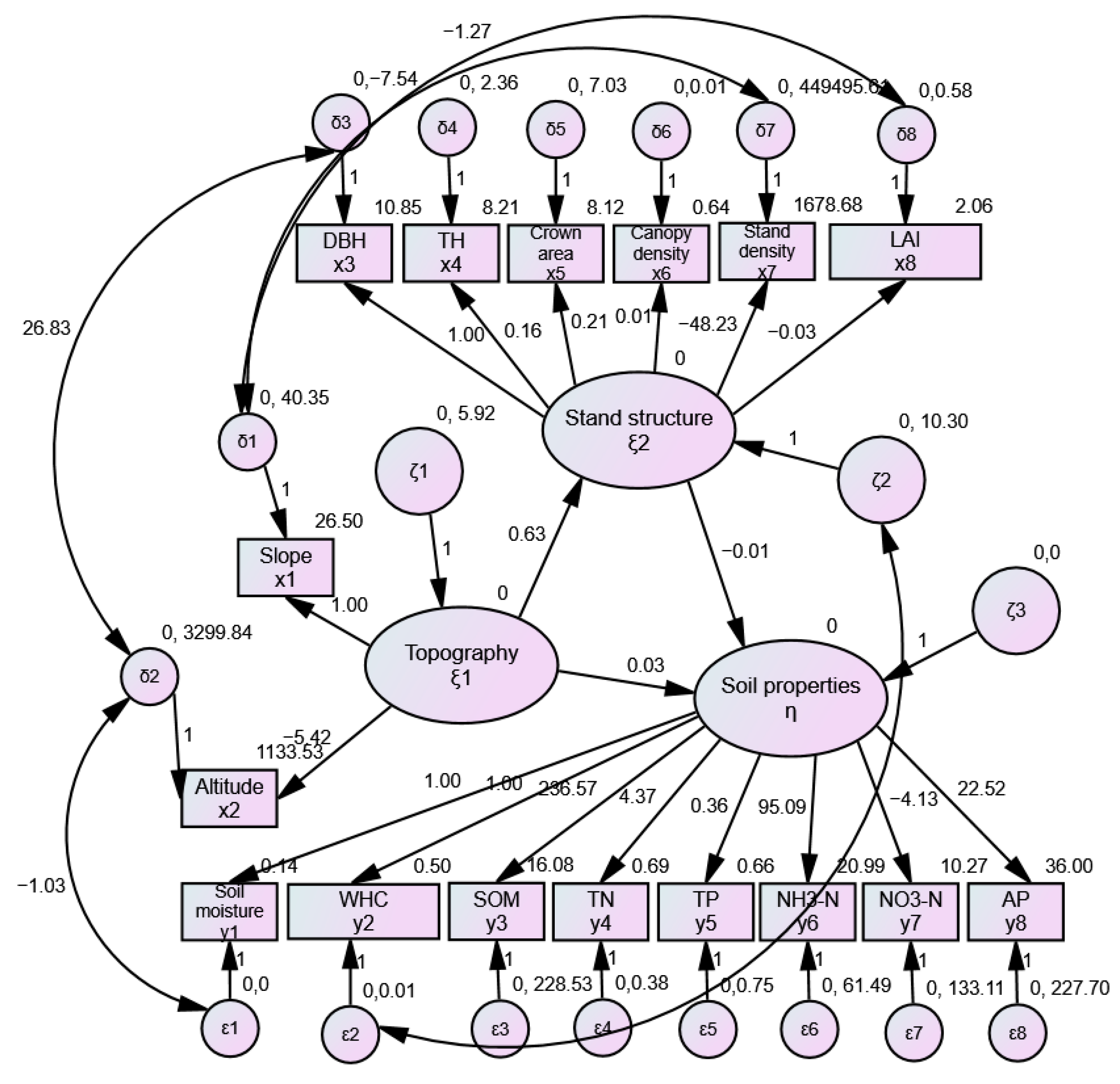
3.1. Model Construction and Correction

SEM has been shown to be verifiable, therefore, the basis for the study of the coupling relationships between stand structure and soil properties was taken into consideration when building the model. The data in this research conformed to a multivariate normal distribution, and maximum likelihood estimation was used to quantitatively analyze potential and observed variables. SPSS 19.0 software (IBM/International Business Machines Corporation, Armonk, NY, USA) was used for data exploratory analysis. Using Amos 22.0 software (IBM/International Business Machines Corporation, Armonk, NY, USA) for drawing the path map and parameter estimation, the path coefficient between each variable, the factor load of each variable, the measurement error of observed variables, and the residual of potential variables could all be obtained.

The initial model was constructed based on generally-known experience. After running in Amos, the chi-square (${\chi }^2$) test statistic value was 414.592 with 101 $df$, and a significant probability (p) value of 0.0001 (<0.05) in the model (Figure 1), which resulted in the rejection of the null hypothesis. The root meant square error of approximation (RMSEA) was 0.152, under the null hypothesis of “close fit” (i.e., RMSEA is no greater than 0.05), as such, the adaptability of the hypothetical model to the observed data should be modified (

Table 3. The fitting parameters describing the coupling relationship between stand structure and soil properties of artificial mixed forests in the Caijiachuan Watershed.

Index Name	Evaluation Criterion	Initial Model	Modified Model
The chi-square (${\mathit{\chi }}^{\mathbf{2}}$)	The smaller the better.	414.592	247.554
The ratio of chi-square and freedom (${\mathit{\chi }}^{\mathbf{2}}/\mathit{d}\mathit{f}$)	1~3. When the ratio is less than 1, the model is over adapted; when the ratio is between 1 and 3, the model is well adapted; when the ratio is greater than 3, the model is poorly fitted.	4.105	2.782
Significant probability (p)	>0.05	0.000	0.078
Normative fit index (NFI)	0~1. A value greater than 0.7 is acceptable, the closer to 1 the better.	0.421	0.754
Incremental fit index (IFI)	0~1. A value greater than 0.7 is acceptable, the closer to 1 the better.	0.490	0.747
Comparative fit index (CFI)	0~1. A value greater than 0.7 is acceptable, the closer to 1 the better.	0.474	0.734
The root meant square error of approximation (RMSEA)	<0.05. The smaller the better.	0.152	0.045
Akaike information criterion (AIC)	The smaller the better.	516.592	373.554
Bayes criterion (BCC)	The smaller the better.	531.287	391.707

).

According to the current theoretical research and qualitative analyses of the conclusions, the model correction was completed using the “Modification Indices” hints of the Amos software. Principally, adding double arrows could express the correlation between the residuals of each variable, so that the parameters of the model were within an allowable range. After being modified, the chi-square (${\chi }^2$) test statistic value became 247.554 and the degree of freedom ($df$) reduced to 89, with significant probability (p) value of 0.078 (>0.05) in the SEM (Figure 2), which accepted the null hypothesis. The value of RMSEA was 0.045 (<0.05), while normative fit index (NFI), incremental fit index (IFI), and CFI were each greater than 0.7, inside the acceptable range, thus the model could be tolerated. Therefore, the test of the fittest indicators also met the standard, indicating that the fit of the model and the observed data were better after correction (Table 3).

3.2. Model Explanation

3.2.1. Relationship between Latent Variables

The topography had positive effects on the stand structure and soil characteristics (Figure 2), and the path coefficients were 0.63 and 0.03, respectively. Numerically, the effect of topography on the stand structure was far greater than its impact on the soil. The stand structure had a negative impact on soil properties, with a path coefficient of −0.01. Standardized influence coefficients characterized the effects of the latent variables, which were calculated using the SEM method (

Table 4. Standardized influence coefficients of latent variables in the structural equation model of Robinia pseudoacacia and Pinus tabulaeformis mixed plantations in the Caijiachuan Watershed.

Effect Type		Influences
		Topography	Stand Structure
Standardized total impact	Stand structure	0.487
	Soil characteristics	1.303	−0.585
Standardized direct impact	Stand structure	0.487
	Soil characteristics	1.589	−0.585
Standardized indirect impact	Stand structure
	Soil characteristics	−0.285

). The impact coefficient of topography on soil characteristics was 1.303, with a direct impact of 1.589 and an indirect impact of −0.285; the total impact and direct impact coefficients of stand structure on soil properties were both −0.585; and the total impact and direct impact coefficients of topography on stand structure were both 0.487.

This showed that, after optimizing the stand structure, soil moisture and nutrients should be slightly influenced. In practice, the stand structure should be optimized as much as possible so as to increase the ecological function of stand. Simultaneously, the moderate stand structure adjustments should also be observed in order to avoid heavier constraints for the soil water resources and fertility when the negative impacts accumulate to a certain extent.

3.2.2. Relationship between Latent and Observed Variables

The extent and effect of the influence between latent variables and observed variables were also reflected in the calculation of the path coefficient of the fit model (Figure 2). First, among the observed variables affecting the topographic factors, the slope showed a positive effect, but the altitude showed an opposite effect, which had a great influence on the topographic factors from a numerical point of view. Second, in the observed variables of influencing the stand structure, DBH, TH, crown width, and canopy density showed positive effects, whereas stand density and LAI both showed negative effects. The effect of stand density on the stand structure was much greater than the other factors. Third, among all of the observed variables that affected soil properties, all of them showed positive effects, except NO₃-N, and the order of their impacts on soil characteristics were: SOM > NH₃-N > AP > TN > soil moisture > WHC > TP (Figure 2).

4. Discussion

The concept of SEM has been applied to many multivariable coupling studies in the natural sciences and has achieved good results in forest ecology studies. Application studies in forests [12,14,42,43], shrublands [13], wetlands [35], and other ecosystems [15] have proved the scientific basis and reliability of the model. Its importance is that it allows for the detection of topographic, stand structural, and soil characteristic factors that are responsible for structural and functional changes. However, the correct interpretation of these models requires a strong supply of ecological data and a good understanding of the characteristics of the topography–stand–soil system.

4.1. Topography Mainly Impacted Stand Structure

Topographical indicators commonly incorporate slope, aspect, altitude, slope length, and slope position, while the basal impacting factors of stand structure were DBH, TH, crown area, canopy density, stand density, forests diversity, LAI, and so on. Different topographic factors influenced forest diversity, structure, and dynamic change by their respective influencing mechanisms as supported by previous research that has demonstrated some aspects of these observations. For instance, tree height had a remarkable dissimilarity based on the slope and aspect of sites [44]; there was significant interaction between aspect and elevation in influencing forest structure [45]; and the vegetation should be adapted to various elevations according to relevant temperatures and other conditions [46].

Examining the data of the mixed plantation, a path coefficient of 0.63 illustrated that the effect of topography on the stand structure was the most important positive factor in the complex relationships. Standardized influence coefficients characterized the effects of the latent variables between topography and stand structure (Table 4). The total impact coefficient of the topography on the stand structure was 0.487, all of which was attributed to direct impacts. Both of the results above demonstrated that if the conditions of the topography in an area became more advantageous, the stand structure can grow more favorably.

In addition to representing the corresponding latent variables, observational variables indirectly affected other related latent variables and further revealed the indirect relationship between the latent variables [42]. The interactive relationship between the observed variables could preferably show the focus of the interaction among the systems represented by the latent variables and explain the current relationship of the latent variables more deeply. Observed variables such as DBH, TH, crown width, canopy density, stand density, and LAI, could not only characterize the stand structure, with the impact coefficients of 1.407, 0.424, 0.305, 0.234, −0.243, and −0.070, but also relate to the topographical factors, with the impact coefficients reaching 0.686, 0.277, 0.144, 0.114, −0.119, and −0.034 (

Table 5. Standardized influence coefficients between observed variables and latent variables in the structural equation model of Robinia pseudoacacia and Pinus tabulaeformis mixed plantations in the Caijiachuan Watershed.

Observed Variables	Influences
	Standardized Total Impact			Standardized Direct Impact			Standardized Indirect Impact
	Topography	Stand Structure	Soil Characteristics	Topography	Stand Structure	Soil Characteristics	Topography	Stand Structure	Soil Characteristics
Slope	0.342			0.342
Altitude	−0.317			−0.317
DBH	0.686	1.407			1.407		0.686
Tree height	0.207	0.424			0.424		0.207
Tree crown area	0.149	0.305			0.305		0.149
Canopy density	0.114	0.234			0.234		0.114
Stand density	−0.119	−0.243			−0.243		−0.119
LAI	−0.034	−0.070			−0.070		−0.034
Soil moisture content	1.117	−0.502	0.857			0.857	1.117	−0.502
WHC	0.546	−0.245	0.419			0.419	0.546	−0.245
SOM	0.732	−0.329	0.561			0.561	0.732	−0.329
TN	0.306	−0.138	0.235			0.235	0.306	−0.138
TP	0.052	−0.023	0.040			0.040	0.052	−0.023
NH3-N	0.547	−0.245	0.419			0.419	0.547	−0.245
NO3-N	−0.088	0.040	−0.068			−0.068	−0.088	0.040
AP	0.043	−0.019	0.033			0.033	0.043	−0.019

Note: In the table, DBH is the abbreviation for diameter at breast height; LAI is the acronym for leaf area index; WHC is the abbreviation for soil maximum water holding capacity; SOM is the acronym for soil organic matter; TN is the is the acronym for total nitrogen; TP is the acronym for total phosphorus; NH₃-N is the acronym for ammonia-nitrogen, NO₃-N is the acronym for nitrate-nitrogen; and AP is the acronym for available phosphorus.

). As such, a deeper relationship between the indicators of the stand structure and the topographic factors could be clearly distinguished among them. The results showed that if the values of DBH, TH, crown area and canopy density were greater then the stand structure was more favorable; conversely, the direct influence of stand density and LAI on the stand structure was negative. Analogously, the indirect influence coefficients between the DBH, TH, crown area, canopy density, and topography were positive, but the others were negative.

4.2. Topography Significantly Influenced Soil by Stand Structure Indirectly

The soil characteristics studied in this paper were soil moisture content, WHC, SOM, TN, TP, NH₃-N, NO₃-N, and AP. The relation of one or several dimensions of these soil characteristics to topography have been found in past research. Slope has been shown to influence antecedent soil moisture which can potentially lead to either an increase or decrease in soil erosion, and is therefore a crucial consideration for recommending appropriate measures to protect soils [47]; there were some significant effects of altitudinal zone and slope aspect on the vertical distribution of soil organic carbon (close to SOM) density [48]. Topography usually has some form of direct impact on soil and, here, topography influenced soil indirectly via stand structure.

Topography had positive effects on the soil characteristics, with a path coefficient of 0.03 (Figure 2), which was a small absolute value. The most influential factor on soil characteristics was topography, with a total impact coefficient of 1.303; the direct impact being positive, and the indirect impact being negative (Table 4). This indicated that the majority of its impact on soil properties was through an indirect impact by influencing the stand structure. Through the stand structure adjustment, the topographic factors might change the formation of soil moisture and nutrients.

In addition to the representation of topography, the observed indicators, such as slope and elevation, were also related to soil characterization, and every factor of the soil characteristics had a positive impact on the topography, except for NO₃-N. The absolute value of the influence coefficient of soil water content on the topographical factors was 1.117, indicating that the impact of the factor on soil moisture was quite high. The values of TP and AP were only 0.052 and 0.043, respectively, showing that the impact of phosphorus was weaker than the other factors’ impacts on the topography. The results of this study align with other recent research that suggests that soil moisture content was the key factor for study site conditions and the status of stand structure. In the future, soil nutrient-related variables, such as organic matter, nitrogen, and phosphorus, should also be given special consideration.

4.3. Stand Structure Impacted Soil Properties to a Comparatively Smaller Degree

The relationships of the stand structure and soil properties were the essential issues. There have been many studies on these factors in the field of ecological systems and soil and water conservation. Soil variables have been observed to differ in terms of soil TN across the different canopy types [49]. Forest structure has effects on microbiological soil properties and nutrient content [50]; however, a great many of these effects still remain in the realm of single-factor impact research. Additionally, using the SEM method to explore the multi-factors, we found that the stand structure impacted soil properties with a path coefficient of −0.01. The total impact coefficient of stand structure on soil properties was −0.585, all of which was attributed to direct impacts. The results indicated that, under the suitable conditions of topographic factors, the stand might negatively impact soil moisture and nutrient conditions.

The effects of the observed variables on latent variables are also described in Table 5. Soil moisture content, WHC, SOM, TN, TP, NH₃-N, NO₃-N, and AP were related to stand structure, apart from the representation of soil characterization. Here, stand structure had a positive relationship to NO₃-N, but it had negative influence coefficients with all of the other soil factors, along with a small absolute value. Soil moisture content was most sensitive, with an influence coefficient of −0.502 on the stand structure. Adversely, the values of TP and AP were −0.023 and −0.019, demonstrating that phosphorus was weakly influenced by the stand structure. These results verify that the benefits of studying stand and soil moisture in an arid area are great, and that the soil nutrients also play a significant and crucial role in forest stand research.

5. Conclusions

The soil characteristics of R. pseudoacacia and P. tabulaeformis mixed plantations in the Caijiachuan Watershed were mainly limited by factors such as the regional topography and the stand structure; SEM satisfactorily quantified the relationships between these factors. The modeling indicated that if the topography was more suitable and the stand structure was more favorable then soil moisture and fertility conditions would be better. This finding was consistent with the initial empirical assumption [1,2,3,4,5,6,7,47,50], with the results of this study offering a more statistically accurate expression than previously determined. The stand structure had little effect on soil properties, all of which were negatively and directly affected, indicating that it imposed certain restrictions on the retained moisture and nutrients in the soil. Observed variables also correlated well with the latent variables. The mutual indirect influences between the observed variables and the two latent variables of topography and stand structure were comparatively high.

Based on all the above, the quantification process should provide new insights into the management and conservation of forests. In line with the quantified effective values of impact between these interrelated factors, some measures may in fact adjust terrain and stand structure to effectively maintain or increase the soil moisture and nutrient content in reality, such as changing the gradient of micro-topography, or reducing the stand density. These measures could enhance the functions of soil and water conservation. In the Loess Plateau, the conservation and forestry staff can achieve this positive outcome by excavating level steps and fish-scale pits to lessen the slopes or reduce runoff, or by artificial tree-tending in order to change the stand structure according to the path coefficient of the modified model. The results can serve as a reference for determining care and management measures suitable for the R. pseudoacacia and P. tabulaeformis plantations, as well as for controlling the stand structure on the Loess Plateau and improving the region’s soil and water conservation functions.

References

1. Bi, H.X.; Li, X.Y.; Li, J.; Guo, M.X.; Liu, X. Study on suitable vegetation cover on Loess area based on soil water balance. Sci. Silvae Sin. 2007, 43, 17–24. [Google Scholar]
2. Brzostek, E.R.; Dragoni, D.; Schmid, H.P.; Rahman, A.F.; Sims, D.; Wayson, C.A.; Johnson, D.J.; Phillips, R.P. Chronic water stress reduces tree growth and the carbon sink of deciduous hardwood forests. Glob. Chang. Biol. 2014, 28, 2531–2539. [Google Scholar] [CrossRef] [PubMed]
3. Panagos, P.; Borrelli, P.; Poesen, J.; Ballabio, C.; Lugato, E.; Meusburger, K.; Montanarella, K.; Alewell, C. The new assessment of soil loss by water erosion in Europe. Environ. Sci. Policy 2015, 54, 438–447. [Google Scholar] [CrossRef]
4. Li, S.; Liang, W.; Fu, B.J.; Lv, Y.H.; Fu, S.Y.; Wang, S.; Su, H.M. Vegetation changes in recent large-scale ecological restoration projects and subsequent impact on water resources in China’s Loess Plateau. Sci. Total Environ. 2016, 569, 1032–1039. [Google Scholar] [CrossRef] [PubMed]
5. Zhang, X.; Zhao, W.W.; Liu, Y.X.; Fang, X.N.; Feng, Q. The relationships between grasslands and soil moisture on the Loess Plateau of China: A review. Catena 2016, 145, 56–67. [Google Scholar] [CrossRef]
6. Shi, W.Y.; Du, S.; Joseph, C.M.; Guan, J.H.; Wang, K.B.; Ma, M.G.; Norikazu, Y.; Ryunosuke, T. Physical and biogeochemical controls on soil respiration along a topographical gradient in a semiarid forest. Agric. For. Meteorol. 2017, 247, 1–11. [Google Scholar] [CrossRef]
7. Wang, Y.H.; Yu, P.T.; Wang, J.Z.; Xu, L.H.; Karl, H.F.; Xiong, W. Multifunctional forestry on the Loess Plateau. Earth Environ. Sci. 2017, 4, 79–107. [Google Scholar]
8. Zhang, C.; Wang, Z.G.; Ling, F.; Ji, Q.; Meng, F.B. Function evaluation of soil and water conservation and its application in soil and water conservation regionalization. Sci. Soil Water Conserv. 2016, 14, 90–99. [Google Scholar]
9. Pimentel, D.; Harvey, C.; Resosudarmo, P.; Sinclair, K.; Kurz, D.; McNair, M.; Crist, S.; Shpritz, L.; Fitton, L.; Saffouri, R.; et al. Environmental and Economic Costs of Soil Erosion and Conservation Benefits. Science 1995, 267, 1117–1123. [Google Scholar] [CrossRef] [PubMed]
10. Grace, J.B. The factors controlling species density in herbaceous plant communities: An assessment. Perspect. Plant Ecol. Evol. Syst. 1999, 2, 1–28. [Google Scholar] [CrossRef]
11. Grace, J.B.; Anderson, T.M.; Smith, M.D.; Seabloom, E.; Andelman, S.J.; Meche, G.; Weiher, E.; Allain, L.K.; Jutila, H.; Sankaran, M.; et al. Does species diversity limit productivity in natural grassland communities? Ecol. Lett. 2007, 10, 680–689. [Google Scholar] [CrossRef] [PubMed]
12. Miao, S.L.; Carstenn, S.; Nungesser, M. Real World Ecology: Large-Scale and Long-Term Case Studies and Methods; Springer: New York, NY, USA, 2009. [Google Scholar]
13. Wang, S.L.; Liang, X.J.; Ma, C.; Zhou, J.P. Coupling relationship between Hedysarum mongdicum shrub plantation and sand soil based on structural equation model. J. Beijing For. Univ. 2017, 39, 1–8. [Google Scholar]
14. Grace, J.B.; Anderson, T.M.; Olff, H.; Scheiner, S.M. On the specification of structural equation models for ecological systems. Ecol. Monogr. 2010, 80, 67–87. [Google Scholar] [CrossRef]
15. Erin, M.M.; Samiran, B.; Edward, W.B.; Linda, M.H.; Donald, D.H. Structural equation modeling reveals complex relationships in mixed forage swards. Crop Prot. 2015, 78, 106–113. [Google Scholar]
16. Shipley, B. Cause and Correlation in Biology; Cambridge University Press: Cambridge, UK, 2000. [Google Scholar]
17. Jonsson, M.; Wardle, D.A. Structural equation modelling reveals plantcommunity drivers of carbon storage in boreal forest ecosystems. Biol. Lett. 2010, 6, 116–119. [Google Scholar] [CrossRef] [PubMed]
18. Lamb, E.G.; Kennedy, N.; Siciliano, S.D. Effects of plant species richness and evenness on soil microbial community diversity and function. Plant Soil 2011, 338, 483–495. [Google Scholar] [CrossRef]
19. Lamb, E.; Shirtliffe, S.; May, W. Structural equation modelling in the plant sciences: An example using yield components in oat. Can. J. Plant Sci. 2011, 91, 603–619. [Google Scholar] [CrossRef]
20. Laliberté, E.; Tylianakis, J.M. Cascading effects of long-term land-use changes on plant traits and ecosystem functioning. Ecology 2012, 93, 145–155. [Google Scholar] [CrossRef] [PubMed]
21. Chen, D.; Zheng, S.; Shan, Y.; Taube, F.; Bai, Y. Vertebrate herbivore-induced changes in plants and soils: Linkages to ecosystem functioning in a semi-arid steppe. Funct. Ecol. 2013, 27, 273–281. [Google Scholar] [CrossRef]
22. Diouf, A.; Barbier, N.; Lykke, A.M.; Couteron, P.; Deblauwe, V.; Mahamane, A.; Bogaert, J. Relationships between fire history, edaphic factors andwoody vegetation structure and composition in a semi-arid savanna landscape (Niger, West Africa). Appl. Veg. Sci. 2012, 15, 488–500. [Google Scholar] [CrossRef]
23. Matías, L.; Castro, J.; Zamora, R. Effect of simulated climate change on soil respiration in a Mediterranean-type ecosystem: Rainfall and habitat type are more important than temperature or the soil carbon pool. Ecosystems 2012, 15, 299–310. [Google Scholar] [CrossRef]
24. Riseng, C.M.; Wiley, M.J.; Black, R.W.; Munn, M.D. Impacts of agricultural land use on biological integrity: A causal analysis. Ecol. Appl. 2011, 21, 3128–3146. [Google Scholar] [CrossRef]
25. Leithead, M.; Anand, M.; Duarte, L.D.S.; Pillar, V.D. Causal effects of latitude, disturbance and dispersal limitation on richness in a recovering temperate, subtropical and tropical forest. J. Veg. Sci. 2012, 23, 339–351. [Google Scholar] [CrossRef]
26. Virginia, C.; Madhur, A. Assessing ecological integrity: A multi-scale structural and functional approach using Structural Equation Modeling. Ecol. Indic. 2016, 71, 258–269. [Google Scholar]
27. Desrochers, R.E.; Kerr, J.T.; Currie, D.J. How, and how much, natural cover loss increases species richness. Glob. Ecol. Biogeogr. 2011, 20, 857–867. [Google Scholar] [CrossRef]
28. Gazol, A.; Tamme, R.; Takkis, K.; Kasari, L.; Saar, L.; Helm, A.; Pärtel, M. Landscape- and small-scale determinants of grassland species diversity: Directand indirect influences. Ecography 2012, 35, 944–951. [Google Scholar] [CrossRef]
29. Santibáñez-Andrade, G.; Castillo-Argüero, S.; Vega-Peña, E.V.; Lindig-Cisnerosc, R.; Zavala-Hurtado, J.A. Structural equation modeling as a tool to develop conservation strategies using environmental indicators: The case of the forests of the Magdalena river basin in Mexico City. Ecol. Indic. 2015, 54, 124–136. [Google Scholar] [CrossRef]
30. Xu, Z. Study on Ecological Function Evaluation and Biodiversity of Typical Forest Stands in Jinxi of the Loess Plateau. Master’s Thesis, Beijing Forestry University, Beijing, China, 2014. [Google Scholar]
31. Quinn, G.P.; Keough, M.J. Experimental Design and Data Analysis for Biologists; Cambridge University Press: New York, NY, USA, 2002. [Google Scholar]
32. Ruiz, M.A.; Pardo, A.; San Martín, R. Structural equation models. Psychol. Roles 2010, 31, 34–45. [Google Scholar]
33. Schumacker, R.E.; Lomax, R.G. A Beginner’s Guide to Structural Equation Modeling; Taylor and Francis Group, LLC: Mahwah, NJ, USA, 2004. [Google Scholar]
34. Valdés, A.; García, D. Direct and indirect effects of landscape change on the reproduction of a temperate perennial herb. J. Appl. Ecol. 2011, 48, 1422–1431. [Google Scholar] [CrossRef]
35. Sutton-Grier, A.E.; Kenney, M.A.; Richardson, C.J. Examining the relationship between ecosystem structure and function using structural equation modelling: A case study examining denitrification potential in restored wetland soils. Ecol. Model. 2010, 221, 761–768. [Google Scholar] [CrossRef]
36. McCune, B.; Grace, J.B. Analysis of Ecological Communities; MjM Software Design: Gleneden Beach, OR, USA, 2002. [Google Scholar]
37. Bollen, K.A. Structural Equations with Latent Variables; John Wiley & Sons: New York, NY, USA, 1989. [Google Scholar]
38. Joreskog, K.G.; Sorbom, D. LISREL 8 User’s Reference Guide; Scientific Software International: Chicago, IL, USA, 1993. [Google Scholar]
39. Hau, K.T.; Cheng, Z.J. Application and analytical strategies of structural equation modeling. Explor. Psychol. 1999, 19, 54–59. [Google Scholar]
40. Schermelleh, K.; Moosbrugger, H. Evaluating the fit of structural equation models: Tests of significance and descriptive goodness-of-fit measures. Methods Psychol. Res. 2003, 8, 23–74. [Google Scholar]
41. Wu, M.L. Structural Equation Model—The Operation and Application of AMOS; Chongqing University Press: Chongqing, China, 2010. [Google Scholar]
42. Li, H.; Wang, J.K.; Pei, J.B.; Li, S.Y. Equilibrium relationships of soil organic carbon in the main croplands of northeast China based on structural equation modeling. Acta Ecol. Sin. 2015, 35, 517–525. [Google Scholar] [CrossRef]
43. Brahim, N.; Blavet, D.; Gallali, T.; Bernoux, M. Application of structural equation modeling for assessing relationships between organic carbon and soil properties in semiarid Mediterranean region. Int. J. Environ. Sci. Technol. 2011, 8, 305–320. [Google Scholar] [CrossRef]
44. Hanieh, S.; Lalit, K.; Russell, T.; Christine, S. Airborne LiDAR derived canopy height model reveals a significant difference in radiata pine (Pinus radiata D. Don) heights based on slope and aspect of sites. Trees 2014, 28, 733–744. [Google Scholar]
45. Eshetu, Y.; Mike, S.; Mesele, N.; Fantaw, Y. Influence of topographic aspect on floristic diversity, structure and treeline of afromontane cloud forests in the Bale Mountains, Ethiopia. J. For. Res. 2015, 26, 919–931. [Google Scholar]
46. Koichi, T.; Satomi, M. Morphological variations of the Solidago virgaurea L. complex along an elevational gradient on Mt Norikura, central Japan. Plant Species Biol. 2017, 32, 238–246. [Google Scholar]
47. Ziadat, F.M.; Taimeh, A.Y. Effect of rainfall intensity, slope, land use and antecedent soil moisture on soil erosion in an arid environment. Land Degrad. Dev. 2013, 24, 582–590. [Google Scholar] [CrossRef]
48. Tshering, D.; Inakwu, O.A.O.; Damien, J.F. Vertical distribution of soil organic carbon density in relation to land use/cover, altitude and slope aspect in the eastern Himalayas. Land 2014, 3, 1232–1250. [Google Scholar]
49. Ou, Z.Y.; Cao, J.Z.; Shen, W.H.; Tan, Y.B.; He, Q.F.; Peng, Y.H. Understory flora in relation to canopy structure, soil nutrients, and gap light regime: A case study in southern China. Pol. J. Environ. Stud. 2015, 24, 2559–2568. [Google Scholar] [CrossRef]
50. Lucas-Borja, M.E.; Hedo, J.; Cerdá, A.; Candel-Pérez, D.; Viñegla, B. Unravelling the importance of forest age stand and forest structure driving microbiological soil properties, enzymatic activities and soil nutrients content in Mediterranean Spanish black pine (Pinus nigra Ar. ssp. salzmannii) Forest. Sci. Total Environ. 2016, 562, 145–154. [Google Scholar] [CrossRef] [PubMed]
Figure 1. The initial structural equation model (SEM) used in the study. Note: The hypothesized initial model used for predicting topography, stand structure, and soil properties is based on soil and water conservation science. A rectangular box is used for each observed variable, with a measurement error, and the numbers correspond to the standardized path coefficients of the initial model on the single arrows in operation. A value outside of a rectangular box is the mean of the indicator, and a value outside of a round box is the residual error before modification. In the figure, DBH is the abbreviation for diameter at breast height; TH is the acronym for height of tree; LAI is the acronym for leaf area index; WHC is the abbreviation for soil maximum water holding capacity; SOM is the acronym for soil organic matter; TN is the is the acronym for total nitrogen; TP is the acronym for total phosphorus; NH3-N is the acronym for ammonia-nitrogen, NO3-N is the acronym for nitrate-nitrogen; and AP is the acronym for available phosphorus.
Forests 09 00124 g001
Figure 2. The modified model. Note: The numbers correspond to the standardized path coefficients on the single arrows, and to correlation coefficients on the double arrows. A value outside of a rectangular box is the mean of the indicator, and a value outside of a round box is the residual error after modification. In the figure, DBH is the abbreviation for diameter at breast height; TH is the acronym for height of tree; LAI is the acronym for leaf area index; WHC is the abbreviation for soil maximum water holding capacity; SOM is the acronym for soil organic matter; TN is the is the acronym for total nitrogen; TP is the acronym for total phosphorus; NH3-N is the acronym for ammonia-nitrogen, NO3-N is the acronym for nitrate-nitrogen; and AP is the acronym for available phosphorus.
Forests 09 00124 g002