Effect of Vertical Canopy Architecture on Transpiration, Thermoregulation and Carbon Assimilation


Earth and Environmental Sciences Division, Los Alamos National Laboratory, Los Alamos, NM 87545, USA
*
Author to whom correspondence should be addressed.
Forests 2018, 9(4), 198; https://doi.org/10.3390/f9040198
Submission received: 5 March 2018
/
Revised: 3 April 2018
/
Accepted: 9 April 2018
/
Published: 11 April 2018
(This article belongs to the Special Issue Defining, Quantifying, Observing and Modeling Forest Canopy Traits)
Abstract
:Quantifying the impact of natural and anthropogenic disturbances such as deforestation, forest fires and vegetation thinning among others on net ecosystem—atmosphere exchanges of carbon dioxide, water vapor and heat—is an important aspect in the context of modeling global carbon, water and energy cycles. The absence of canopy architectural variation in horizontal and vertical directions is a major source of uncertainty in current climate models attempting to address these issues. This manuscript demonstrates the importance of considering the vertical distribution of foliage density by coupling a leaf level plant biophysics model with analytical solutions of wind flow and light attenuation in a horizontally homogeneous canopy. It is demonstrated that plant physiological response in terms of carbon assimilation, transpiration and canopy surface temperature can be widely different for two canopies with the same leaf area index (LAI) but different leaf area density distributions, under several conditions of wind speed, light availability, soil moisture availability and atmospheric evaporative demand.
1. Introduction
Carbon, water and biogeochemical cycles of forest ecosystems are critically important in determining Earth’s energy balance. Resolving the role of the biosphere as a terrestrial carbon sink and the nature of nonlinear couplings between these cycles across a very wide range of spatiotemporal scales (stomata to landscape; seconds to days) constitute the scope of modeling work identified by the Department of Energy’s (DOE) Next Generation Ecosystem Experiments (NGEE) project [1]. The NGEE Tropics campaign aims to identify major scientific issues such as (1) effects of changing patterns of temperature, precipitation and carbon dioxide () on tropical forests; (2) disturbances effects on ecosystem exchanges—i.e., how carbon, water and energy fluxes are impacted by vegetation thinning, insect outbreaks, land use change, forest fires etc. Answering these questions requires moving beyond the big leaf approximation of vegetation canopies prevalent in large scale models [2]. Reducing the three dimensional canopy into one single layer certainly has computational benefits but completely misses the complexity arising out of the spatial variation of plant functional traits [3]. Capturing the effects of disturbances thus require considering the horizontal and vertical variation of canopy architecture since plant-atmosphere interactions have several nonlinear dependencies with the canopy microclimate parameters that are altered significantly with variations of the spatial structure of the canopy. The temperature of the canopy is another important factor that governs enzyme reactions, membrane transport etc. among other physiochemical activities and also can be taken as an indicator of plant health. Although some earlier studies had used air temperature as a proxy for plant temperature, it is well established now that plant temperature can deviate from air temperature following the physical processes of transpiration and heat transfer. This process of modulating plant temperature based on the economics of carbon, water and heat exchange is called thermoregulation [4,5].
The response of plants to abiotic stressors emerges from the complex nonlinear interactions among several physiological and environmental parameters such as stomatal conductance, water use efficiency, light availability, wind speed, relative humidity, and ambient concentration [6]. The presence of edges and clearings (gaps) inside the canopy disturbs the constant flux layer assumption in the canopy sub layer and changes wind flow patterns by creating small recirculation zones [7,8]. While the edge problem requires considering the variations of canopy structure in the horizontal directions, variation of canopy architecture in the vertical dimension alone is sufficient to generate different plant response to varying micrometeorological parameters. Katul et al. [9] demonstrated the systematic variation of turbulence statistics inside vegetation canopies across a wide range of leaf area density (LAD) distributions. Different LAD distributions also generate varied light environments inside the canopy [10]. There have been several theoretical and experimental studies on the effect of elevated on LAI, which is a representative parameter of plant foliage density and can be taken as an index for plant health [11,12,13]. Under increased concentration, plants may undergo more photosynthesis and if they are able to uptake nutrients from the soil, the availability of excess carbohydrates can help them build tissue, thereby increasing LAI. Increased also leads to lower stomatal conductance. In plant canopies that are well coupled to the atmosphere, this decrease in stomatal conductance by stomatal closure leads to water savings, which also increases LAI. However, increased LAI simultaneously leads to lower light availability, as well as lower throughfall precipitation and wind speed, which reduces LAI potentially enough to offset any gains achieved by other mechanisms over time. If the canopy is not well coupled to the atmosphere, there is lower water savings because of lower boundary layer conductance in spite of reduced stomatal conductance, leading to minimal effects on LAI. Moreover, during drought-like conditions, the marginal water use efficiency will increase and the combination of low soil moisture availability and higher vapor pressure deficit (VPD) reduces stomatal conductance further (on top of reduced stomatal conductance from elevated ). This could lead to negative carbon balances for individual leaves causing the plant to shed leaves (called `leaf-out’) and reduce LAI [13]. The higher daytime leaf temperature due to reduced stomatal conductance also causes a slowdown in low-temperature acclimation, reducing the plant’s resilience to cold temperature [14,15,16,17]. Thus, the future health of the plant under elevated concentrations, hot drought and irregular warm-cold cycles depends on the interplay of a variety of micrometeorological factors with plant physiology across the landscape.
Resolving the full complexity of the problem is numerically and computationally intractable due to the myriad of scales in space and time, as well as the complicated nonlinear feedback loops between several processes in the soil-plant-atmosphere continuum. Hence low dimensional predictive frameworks need to be developed to capture the essential modes of variability between modules to approximate the system. The current work uses such a model which can solve plant atmosphere exchange processes at the leaf level and systematically explores the effect of vertical canopy architectural variation on canopy transpiration, carbon uptake and thermoregulation. Two different vertical foliage distributions (in the form of leaf area density or LAD) are explored for the same LAI. The first one is top heavy—meaning most of the foliage are concentrated at the top and the other one is bottom heavy—meaning most of the foliage are concentrated at the bottom, representing two end cases of foliage distribution. Note that the integrated vertical profiles of both LAD profiles yield the same LAI. Transpiration, carbon uptake and thermoregulation are chosen since these processes represent the fluxes of water, carbon and heat which control the corresponding water, carbon and energy cycles. The variations of plant physiological response for the same canopy LAI but with different LAD distributions across a multitude of water supply and demand conditions will highlight the importance of capturing canopy architecture in models aimed at quantifying ecosystem-atmosphere interaction.
2. Theory
The plant biophysics model is a culmination of several different studies of plant functionality, which have been compiled by Huang et al. [18]. Earlier versions of the model can be found in several works such as Katul et al. [13], Launiainen et al. [19], Siqueira et al. [20] and Lai et al. [21]. The framework is based on the following principles: (1) a model for the biochemical demand for as prescribed by photosynthesis models. This model can differentiate between photosynthesis under light-limited and nutrient-limited scenarios; (2) A Fickian mass transfer model including transfer through the laminar boundary layer on leaves that may be subjected to forced or free convection depending upon the mean velocity and the radiation load; (3) an optimal leaf water use strategy that maximizes net carbon gain for a given transpiration rate to describe the stomatal aperture variation; (4) a leaf-level energy balance to accommodate evaporative cooling. The model can be adapted for both amphistomatous (stomates on both sides) and epistometous leaves (stomates on one side). Leaf-level models using the aforementioned philosophies are upscaled to plant, canopy and landscape scales using one dimensional analytical solutions for mean flow inside vegetation canopies.
Leaves uptake carbon dioxide through stomata during the process of photosynthesis. However, loss of water also takes place through the open stomata during the process of carbon assimilation. So the plant needs to optimize these two processes by controlling the stomatal apertures. Moreover, the presence of a laminar boundary layer over the leaf surface further complicates the problem by decoupling the leaf from the atmosphere. The thickness of this boundary layer controls the diffusive path length for gas exchange between the leaf and the turbulent atmosphere beyond the laminar boundary layer. The thermodynamics of heat exchange and evaporative cooling is also dependent on the wind speed, radiation load, air temperature, relative humidity etc.
The current model resolves these biotic controls through stomatal response to the turbulent atmosphere by encoding more physical processes compared to existing models. The main advancements are using a leaf boundary layer modulating level exchange and using an optimization strategy based on carbon and water economies of the leaves [18].
2.1. Fickian Mass Transfer Model
The assimilation of carbon dioxide happens as a flux between the leaf and the atmosphere through the laminar boundary layer on the leaves:
Similarly the flux of water vapor from the leaf to the atmosphere can be written as
i denotes intercellular concentration and a denotes ambient concentration. c denotes concentration and e denotes concentration of water vapor. denotes the total conductance which is a combination of both boundary layer () and stomatal () conductance:
2.2. Boundary Layer Conductance
The boundary layer conductance for scalars (i) such as carbon dioxide, heat and water can be written as a combination of conductance under free and forced convection:
Forced convection for heat:
Free convection for heat:
where is the Reynolds number, d is leaf dimension, is kinematic viscosity, is the Prandtl number and is the Grashof number. For carbon dioxide and water, replace with Schmidt number. , where is plant temperature, is air temperature.
2.3. Photosynthesis Model
The Farquhar model of photosynthesis for C3 plants is used [22], which was modified by Vico et al. [23] to ensure a smooth transition between co-limitations of Rubisco limited and light limited photosynthesis:
where and are photosynthesis parameters. is carbon dioxide compensation point. is daytime mitochondrial respiration rate. J is electron transport rate that varies with light availability. and are Michaelis constants for carbon dioxide fixation and oxygen inhibition and is the ambient oxygen concentration. is the maximum carboxylation capacity. All parameters are functions of . For more details, please refer to Huang et al. [18].
2.4. Leaf Level Energy Balance
The energy balance on the leaf surface can be written as
where is the net radiation, is the absorbed radiation, is the outgoing radiation, H is the sensible heat flux and is the latent heat flux. can be modeled using the Stefan-Boltzmann law:
where is the leaf surface emissivity, is the Stefan-Boltzmann constant. The sensible and latent heat flux can be written as
and
where is the specific heat capacity of air and L is the latent heat of vaporization of water and is atmospheric pressure. Rearranging the energy balance equation yields the following implicit equation which needs to be solved numerically.
2.5. Stomatal Optimization Model
The closure for the system of equations is provided by invoking an optimality hypothesis based on the economics of leaf-gas exchange. The short term regulation of stomatal aperture is hypothesized as an optimization process that maximizes carbon gain constrained by water loss. This is a reasonable assumption because plants have to open their stomata to gain carbon dioxide necessary for building tissues. However, the open stomata also results in water loss through transpiration. Thus, the uptake of carbon comes at a cost of losing water. To represent this idea mathematically, a Hamiltonian is constructed to solve the constrained optimization problem.
where is the Lagrange multiplier, called marginal water use efficiency and measures the cost to the plant of losing water in carbon units thereby bridging the carbon and water economies of the plant. One needs to solve numerically for
2.6. Algorithm
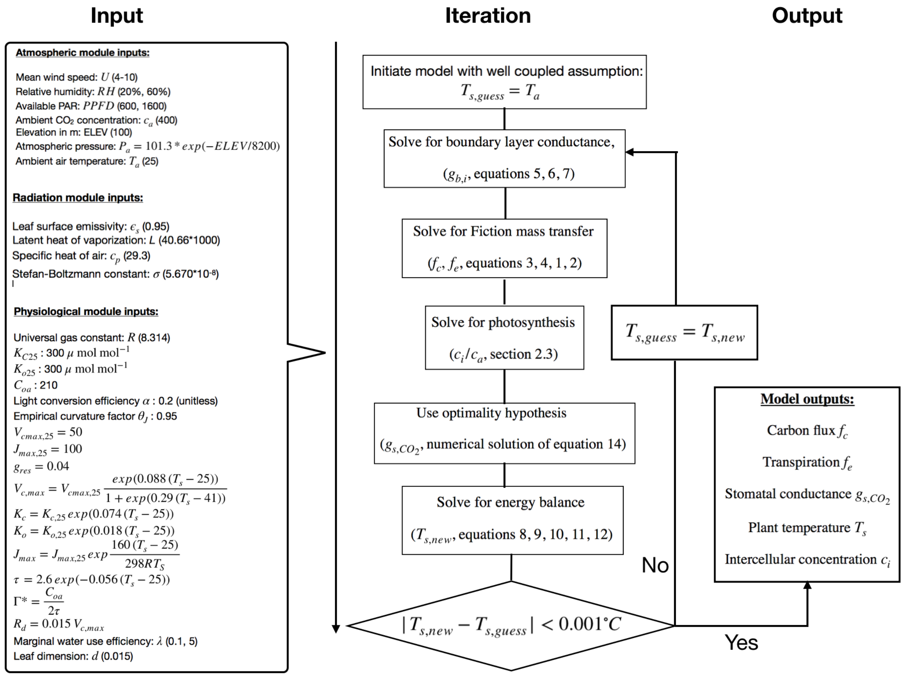
Figure 1 taken from Huang et al. [18] shows the algorithm for the plant biophysics code along with values of input parameters for reproducibility. Essentially one needs to initialize the model with an assumption for plant temperature equal to air temperature (). This allows one to compute the boundary layer conductances and use that information to compute The Fickian mass transfer model along with the photosynthesis model that computes and . In these computations, , the stomatal conductance of , remains unknown. Solving the constrained optimization problem numerically allows one to solve for . After this, one can solve the energy balance equation numerically to solve for the updated value of . This process is repeated in loops until subsequent iterations for converge.
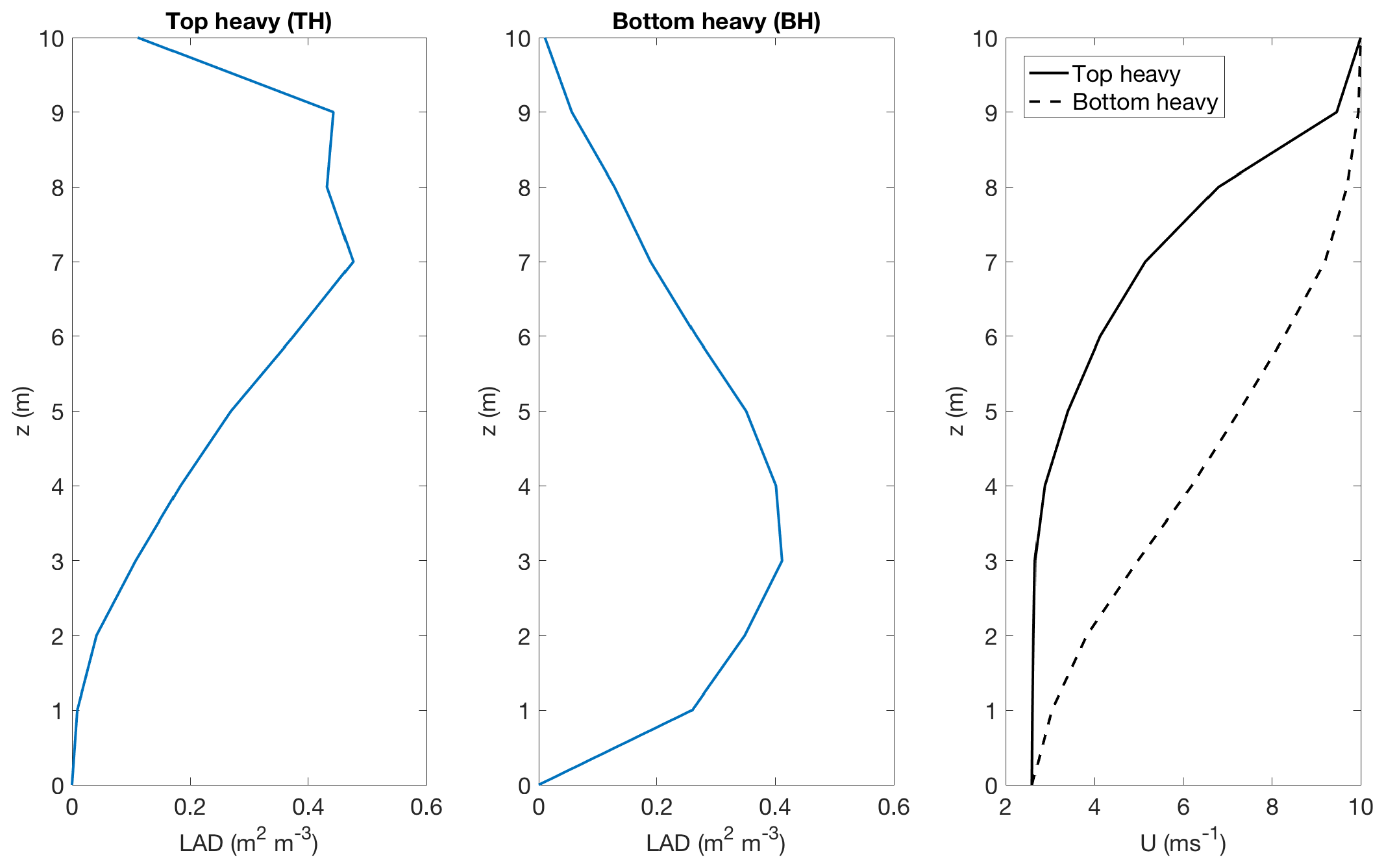
To investigate the effect of wind canopy architecture, we drive the model with a range of wind speed conditions ( to ) prescribed at the canopy top. Canopy response under this range of wind conditions are tested for the two different (two sided) LAD distributions as shown in Figure 2. The left panel shows the top heavy (TH) distribution and the right panel shows the bottom heavy (BH) distribution. Both TH and BH distributions, when integrated, yields the LAI of . The wind speed distribution within the canopy airspace is assumed to attenuate exponentially inside the canopy, following the model of Yi [25]
where is the wind speed at canopy top, h denotes the canopy height (10 m), and is the cumulative leaf area index from ground () to z level. The third panel in Figure 2 shows the mean velocity profile obtained using Equation (15) for the top heavy and bottom heavy cases, for the canopy top wind speed of .
Other input conditions for the model include the air temperature and the ambient concentration of 380 ppm.
Each of these LAD cases are driven by two different light availability conditions— photosynthetically active radiation (PPFD) of 600 and 1600 on top of the canopy. The PPFD profiles are also attenuated inside the canopy following the Beer Lambert law [26]:
where is the PPFD at height z, is the PPFD at canopy top, K is light extinction coefficient and is the cumulative LAI unto height z from top.
Each of these LAD-PPFD combinations are then tested for four different water supply and demand conditions:
- WW RH20: well watered soil () and high evaporative demand in the atmosphere (relative humidity (RH) = );
- WW RH60: well watered soil () and low evaporative demand in the atmosphere (relative humidity (RH) = );
- WS RH20: water stressed soil () and high evaporative demand in the atmosphere (relative humidity (RH) = );
- WS RH60: water stressed soil () and low evaporative demand in the atmosphere (relative humidity (RH) = ).
Once the leaf level outputs are obtained, leaf level fluxes are upscaled to plant scale fluxes by multiplying with leaf area density and grid height at every grid cell. Canopy level fluxes are computed by integrating plant level fluxes for the entire plant volume.
3. Results and Discussions
3.1. Comparison with Published Results
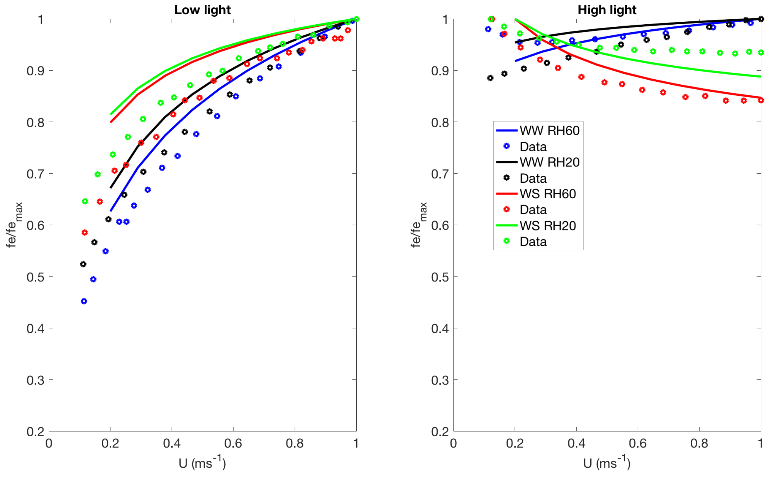
Figure 3 shows the variation of transpiration with respect to wind speeds for the high and low light environments and for each of the four water availability and evaporative demand conditions. The model outcomes are plotted against data plotted in Huang et al. [18], to check if the model development was correct. The difference between the model and the data are because there are uncertainties in some parameters that are not reported in Huang et al. [18] such as absorbed radiation (), which we assume to be twice of PAR. Moreover, we could not use a value of reported by Huang et al. [18] as the numerical solution was found to be unstable. We used a for well watered condition instead. However the correct response in terms of whether transpiration increases or decreases with wind speed is captured, which is deemed more important in the current context. Under low light conditions, transpiration increases with wind speed for all four water supply-demand conditions. However, for higher light conditions, transpiration for only well watered conditions increases with wind speed. Under water stressed conditions, evaporation actually decreases with wind speed for both low and high evaporative demand in the atmosphere. This has been explained by a lowered stomatal conductance because of higher carbon gain. The bottom line is that leaf level physiological response is highly nonlinear and dependent on the local conditions of light availability, wind speed, relative humidity and soil moisture availability among other conditions. The response terms such as carbon and water flux as well as temperature are also interdependent. If enough moisture is present in the soil, there would be high transpiration depending on wind speed, which could help the plant cool down. However, recalling that carbon exchange and water exchange are opposing effects to each other and happen through the same stomatal control, too much carbon gain would lead to stomatal closure because of toxic effects and eventually that might lead to lower transpiration.
3.2. Effect of Canopy Architecture on Transpiration
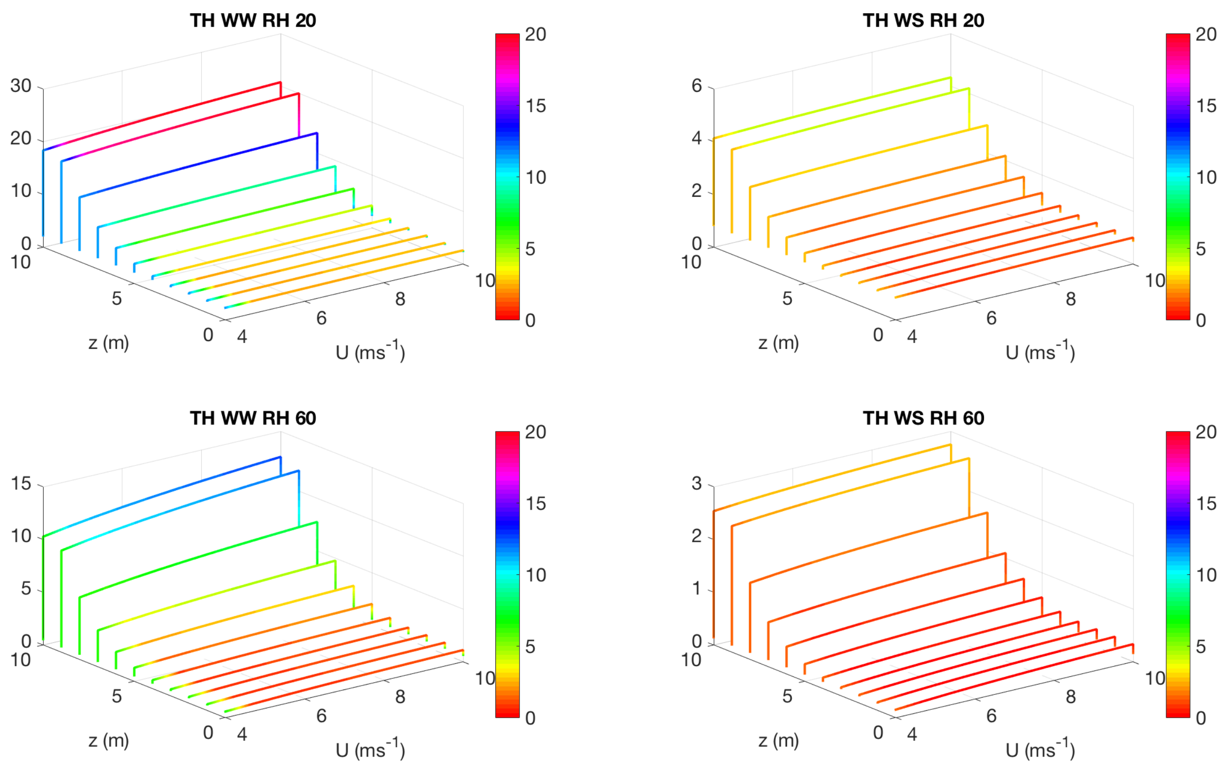
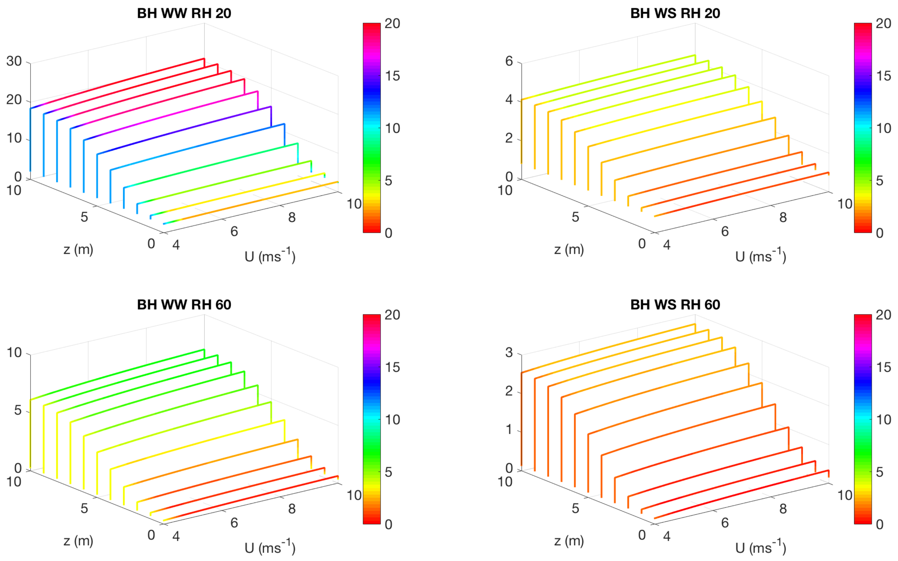
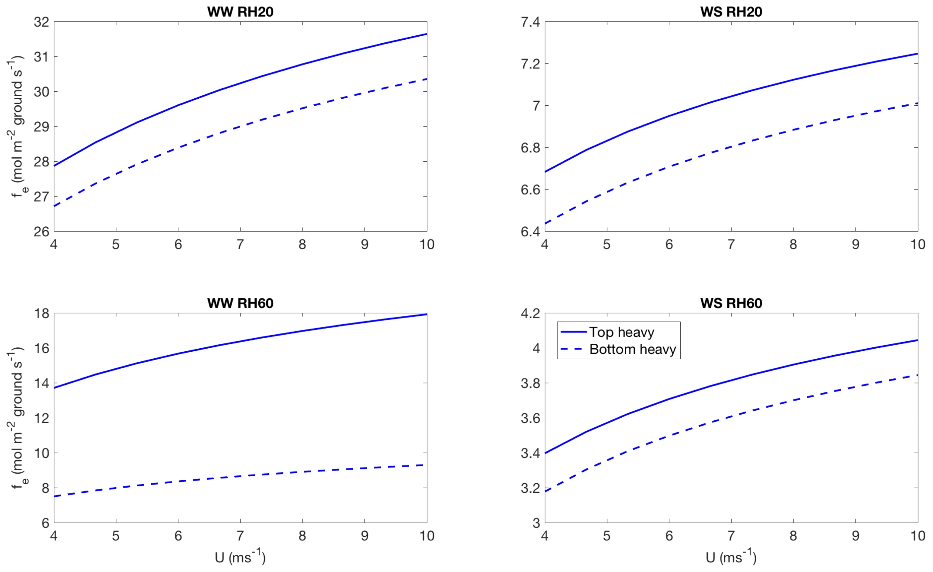
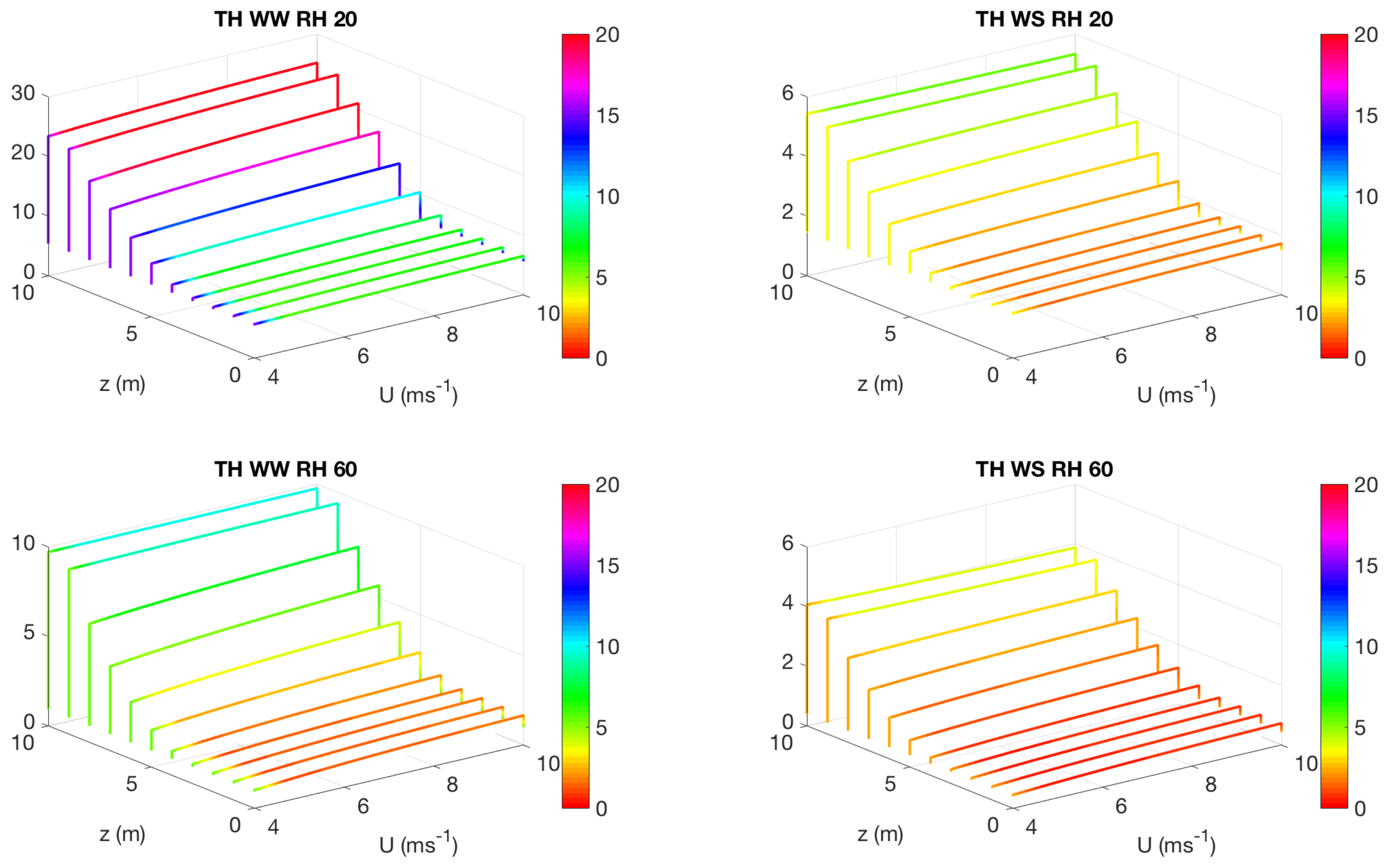
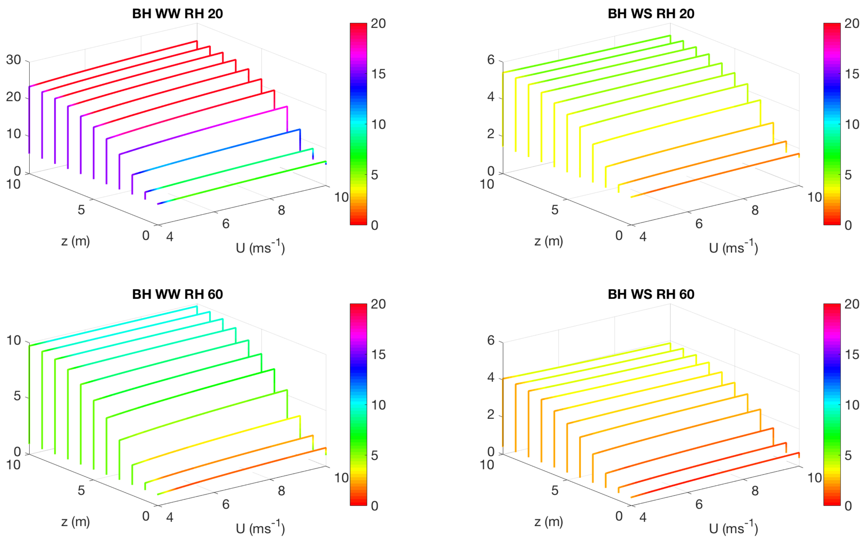
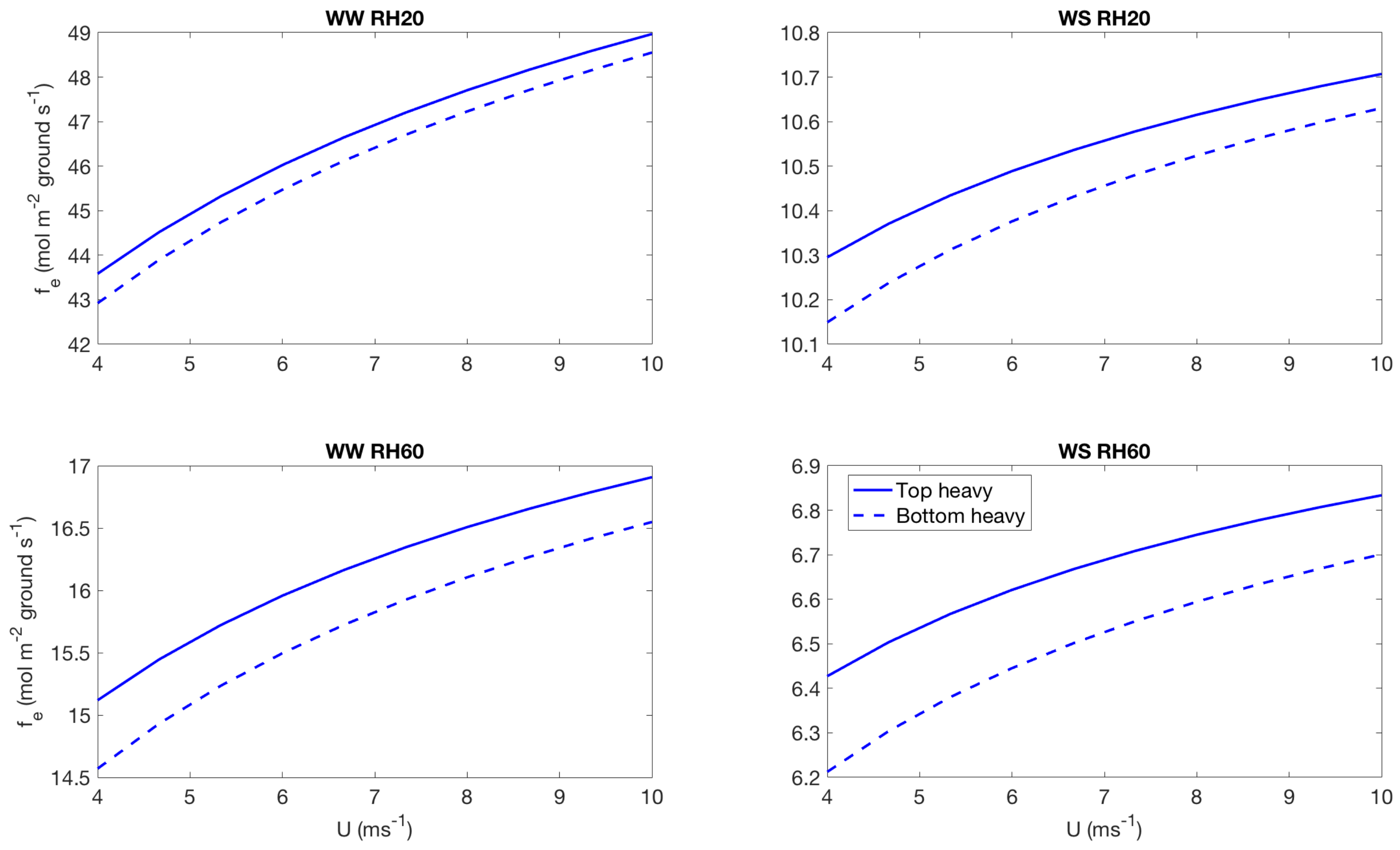
Figure 4 shows the variations of leaf level transpiration with wind speed U and height z for the top heavy (TH) scenario for four different cases in low light conditions. WW indicates well watered and WS indicates water stressed condition. RH20 indicates high evaporative demand (20% relative humidity) and RH60 indicates low evaporative demand in the atmosphere (60% relative humidity). Waterfall figures are used instead of showing heatmaps to identify the wind speed variation of transpiration at individual vertical levels more clearly. Figure 5 shows the same cases for the low light condition but for bottom heavy (BH) scenario. Figure 6 shows the integrated canopy level fluxes for the four cases in the low light condition.
Figure 7 shows shows the variations of leaf level transpiration with wind speed U and height z for the top heavy (TH) scenario for four different cases in high light conditions. Figure 8 shows the same for the bottom heavy scenario. Similar to Figure 6, Figure 9 shows the integrated canopy level transpiration for the four different scenarios for both top heavy and bottom heavy scenario, but for high light conditions.
Several observations can be made from Figure 4, Figure 5, Figure 6, Figure 7, Figure 8 and Figure 9:
- well watered high evaporative demand condition (WW RH20): Transpiration is highest for this condition for both top heavy and bottom heavy scenarios under all light conditions. For the top heavy conditions, the top levels of the canopy undergo higher levels of transpiration and lower levels have significantly less transpiration. For the bottom heavy scenario, the bottom levels undergo considerable transpiration. However canopy level transpirations are higher for the top heavy scenario. Transpiration increases with wind speed for almost all cases both for leaf level and canopy level results, although this is more prominent in the top layers of the canopy. Overall, integrated canopy level transpiration is much higher for the higher light conditions.
- well watered low evaporative demand condition (WW RH60): This scenario always has lower transpiration than the high evaporative demand conditions because of lower demand but has higher transpiration rates compared to the other water stressed conditions because of higher supply of water/moisture. For the top heavy conditions, the top levels of the canopy undergo higher levels of transpiration and lower levels have significantly less transpiration. For the bottom heavy scenario, the bottom levels undergo considerable transpiration. However canopy level transpirations are higher for the top heavy scenario. Transpiration increases with wind speed for almost all cases both for leaf level and canopy level results, however the rate of increase of leaf level transpiration at the top layers are higher than the well watered high evaporative demand condition. Another interesting observation is that for this scenario, the increase of transpiration with wind speed for top heavy and bottom heavy scenarios follows different rates, and the difference is more prominent for the low light conditions. Overall, integrated canopy level transpiration is much higher for the higher light conditions.
- water stressed high evaporative demand condition (WS RH20): This scenario has lower transpiration rates compared to both well watered scenarios because of lower supply of soil moisture. However, the transpiration rate is higher compared to the water stressed, low evaporative demand condition (WS RH60) because of higher atmospheric demand. For the top heavy conditions, the top levels of the canopy undergo higher levels of transpiration and lower levels have significantly less transpiration. For the bottom heavy scenario, the bottom levels undergo considerable transpiration. Canopy level transpirations are higher for the top heavy scenario. Unlike the other scenarios, leaf level transpiration rates remain relatively flat with the increase of wind speed at all levels for the low level condition. For high light conditions, leaf level transpiration actually reduces at the top levels with increase of wind speed. At lower levels, leaf level transpiration still increases with wind speed. Overall canopy level transpiration increases with wind speed but the rate of increase is quite low.
- water stressed low evaporative demand condition (WS RH60): This scenario has lowest transpiration rates among all cases because of lowest supply and lowest demand. For the top heavy conditions, the top levels of the canopy undergo higher levels of transpiration and lower levels have significantly less transpiration. For the bottom heavy scenario, the bottom levels undergo considerable transpiration. Canopy level transpirations are higher for the top heavy scenario. It is interesting to note that for low light conditions, leaf level transpiration at the top layers increase with wind speed but decrease with wind speed at high light conditions. Overall canopy level transpiration still increases with wind speed but at different rates for the top heavy and bottom heavy scenarios.
3.3. Effect of Canopy Architecture on Canopy Temperature
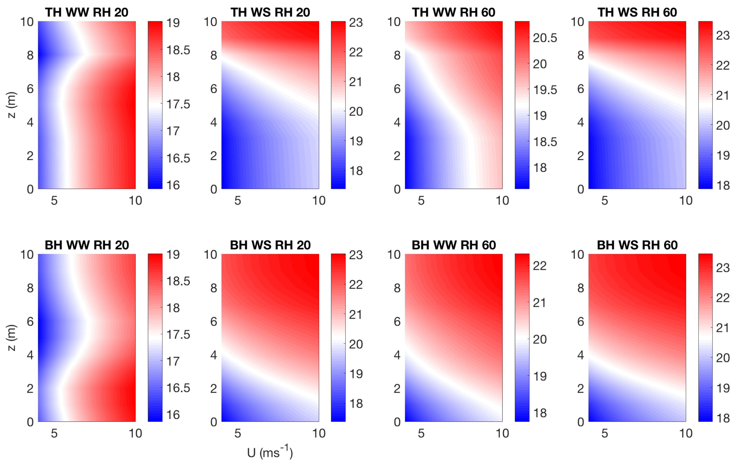
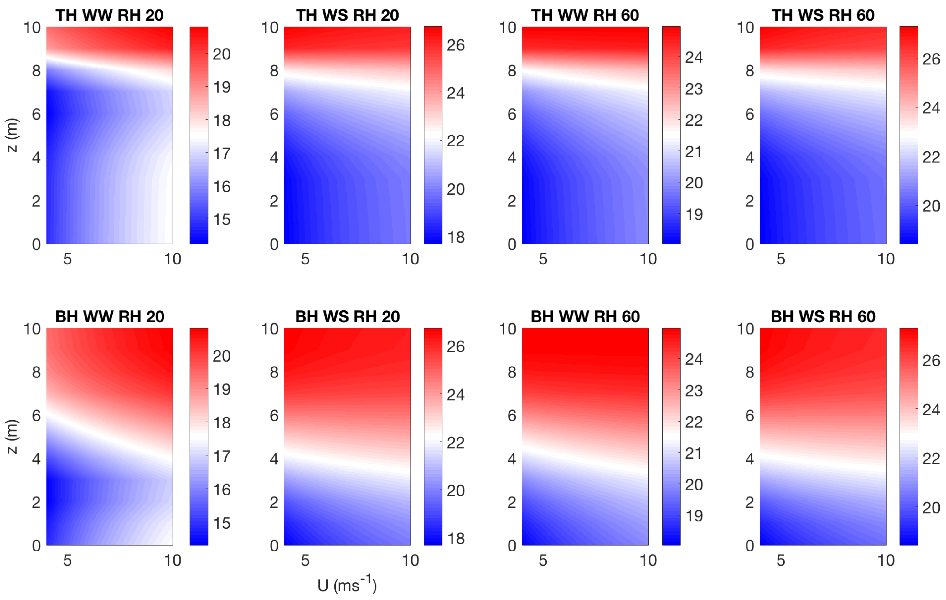
As recognized before from Equation (12), canopy temperature is derived from a solution of leaf level energy balance, which depends on stomatal conductance of heat and water vapor, which in turn depend on the carbon and water fluxes. Figure 10 shows the variation of leaf level temperature with height and wind speed for different water supply and demand conditions for low light level—well watered, high demand (WW RH20); water stressed, high demand (WS RH20); well watered low demand (WW RH60) and water stressed low demand (WS RH60). The top row shows these conditions for the top heavy (TH) scenario and the bottom row for the bottom heavy (BH) scenario. Figure 11 shows the same conditions for the high light level. Several observations can be made from Figure 10 and Figure 11. The well watered high evaporative demand condition (WW RH20) shows lowest temperature across all canopy layers which can be attributed to the highest transpiration rates. The top layers are colder and the middle layers are warmer for this condition for the top heavy case; while the middle layers are colder for the bottom heavy case which can also be attributed to higher transpiration at the middle layers. For the other conditions, more bottom layers of the canopy are warmer for the bottom heavy scenarios for both high and low light conditions. For the top heavy condition, more bottom layers are colder than the top layers for the higher light condition.
4. Effect of Canopy Architecture on Carbon Exchange
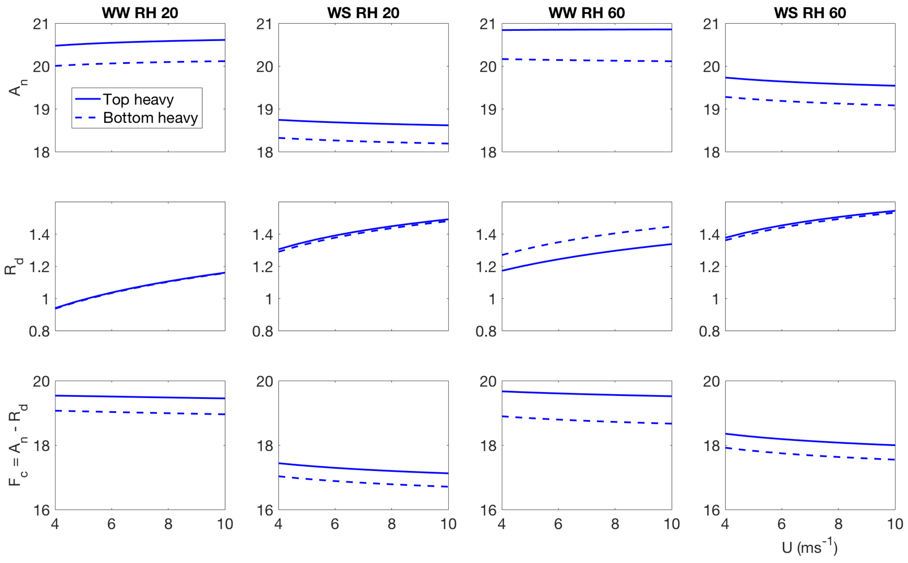
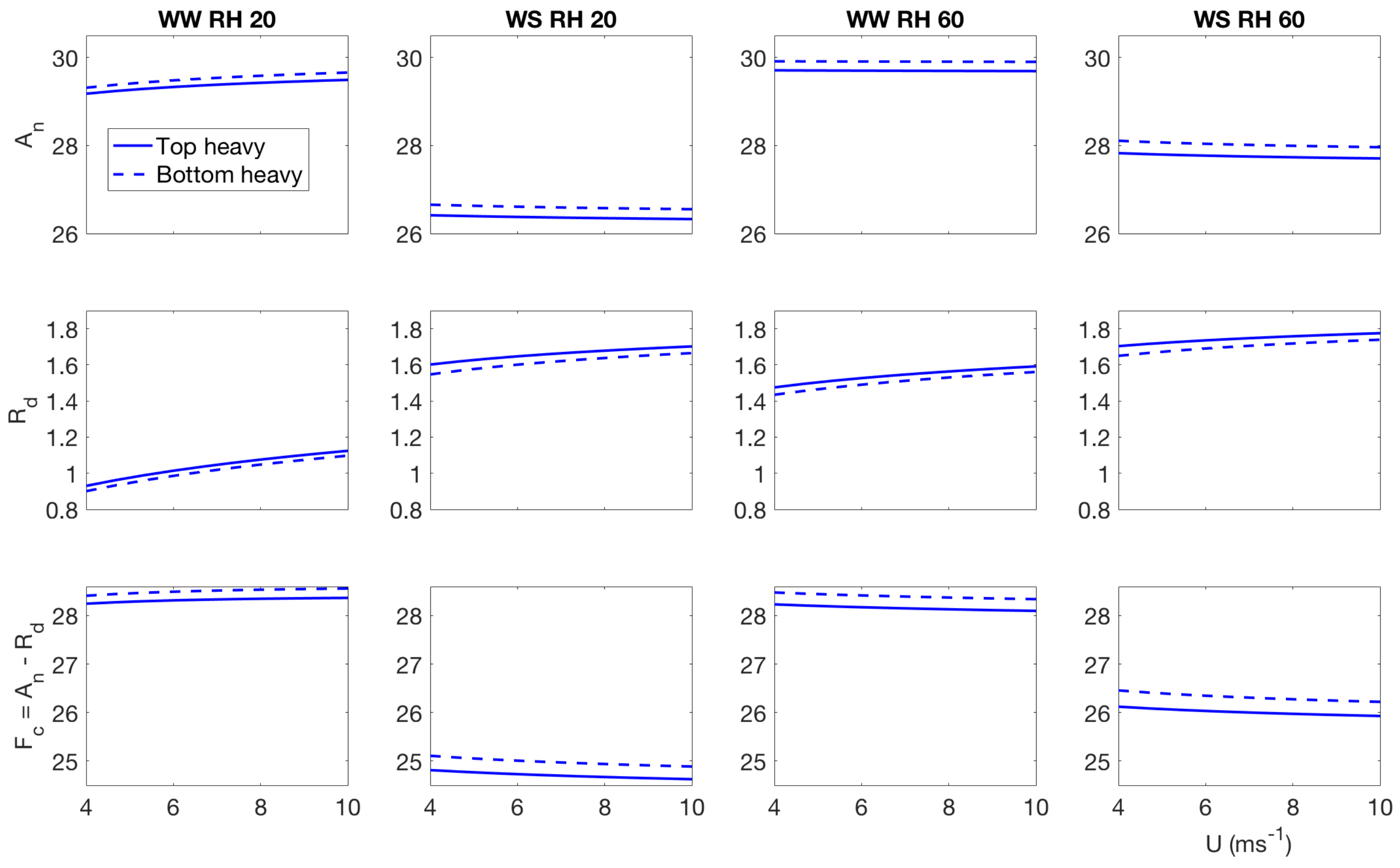
The effects of canopy architecture and water supply and demand conditions on carbon exchange are shown in Figure 12 (low light condition) and Figure 13 (high light condition). The top row shows the net canopy level carbon assimilation , the middle row shows canopy level respiration and the bottom row shows net carbon flux which is given by . Several observations can be made from Figure 12 and Figure 13.
- Well watered, high evaporative demand: carbon assimilation increases slightly with wind speed, however, respiration increases at a faster rate, so effectively net carbon uptake reduces with wind speed at low light condition. The top heavy scenario has higher assimilation and carbon uptake in the low light condition compared to the bottom heavy scenario. In the higher light condition, the bottom heavy scenario has higher carbon assimilation and higher net carbon uptake compared to the top heavy scenario. That said, respiration for the top heavy scenario is higher. More interestingly, the net assimilation and carbon uptake increases with wind speed unlike the low light condition. The difference of behavior can be attributed to different temperature response—which is one of the main driver of the stomatal conductance of carbon dioxide and respiration. Also important to recall the contrasting nature of carbon uptake and water release. The stomates open to maximize carbon gain and minimize water loss. However, when the stomatal apertures are large to satisfy the high transpiration rates, they also gain more carbon. However, these results indicate that under low light conditions, the contrasting effects are still there but in higher light conditions, the stomatal opening is not sufficient enough to impose opposing effects of water loss and carbon gain.
- Water stressed, high evaporative demand: this scenario has the lowest carbon assimilation and uptake, which reduce with wind speed under high and low light conditions. For the low light condition, the top heavy scenario has higher carbon assimilation, respiration and uptake. However, for the higher light condition, the bottom heavy scenario has higher carbon assimilation and uptake with the exception of respiration.
- well watered low evaporative demand: This scenario also has higher rates of carbon assimilation and net uptake and they reduce with increasing wind speed under both high and low light conditions. This scenario also displays the highest differences between the top heavy and bottom heavy scenarios. Like the other cases, the top heavy case has higher carbon assimilation and uptake than the bottom heavy scenario with the exception of respiration. The trend completely reverses under higher light condition.
- water stressed low evaporative demand Under this condition, carbon assimilation and net carbon uptake reduce with wind speed, while the respiration increases in wind speed for both light environments. However, the rate of respiration increase are different under different light conditions. Also interestingly, under low light environment, the top heavy case uptakes more carbon, while under high light conditions, the bottom heavy case uptakes more carbon.
5. Conclusions
In the current manuscript, we investigated the effect of vertical canopy architecture variation on plant physiological response. large scale climate models often use a big-leaf approximation, ignoring the three dimensional structural variation of the canopy. Such models often use the leaf area index (LAI) as a representative proxy for the canopy. We demonstrate that for the same LAI, the transpiration, carbon exchange and canopy temperature would be widely different for two different distributions of leaf area density—one where most of the foliage are concentrated at the top and one where most of the foliage are concentrated at the bottom. A leaf level plant physiological model that considers photosynthesis, leaf level energy balance, Fickian mass transfer between the leaf and atmosphere through a laminar boundary layer on the leaf surface and stomatal optimization is used following the work of many different authors, which was recently compiled by Huang et al. [18]. The leaf level plant physiological model is coupled with analytical solutions of wind flow and light attenuation inside horizontally homogeneous canopies. Leaf level outputs are converted into plant level outputs, which are converted to canopy level outputs by integrating over the canopy height. Leaf and canopy level response under different conditions of wind speed, light availability, soil moisture availability and evaporative demand in the atmosphere are tested and found to be widely different and nonlinear. However, one needs to recall the limitations of the current model, which assumes steady state in flux exchange, neglects the dynamics of subsurface and xylem transport of water flow, as well as the feedback of the canopy level fluxes on the microclimate of the canopy flow itself (local scalar sources and sinks would alter scalar transport in the simulated domain). Moreover, this modeling framework assumes a well coupled canopy with the atmosphere, so that air temperature and carbon dioxide concentrations are considered well mixed and uniform in the sub-canopy space. However, even with this simple model, this demonstration highlights the fact that architectural variation even in one direction can result in significant variations in canopy atmosphere exchange. Any disturbance effect (such as insect outbreak/forest fire etc.) or any management practice such as thinning [27] that changes the local structure of the canopy will lead to a new regime of sub canopy microclimate—which will be manifested by changes in local wind speed, local light availability and local moisture availability among other factors. These changes will in turn alter the canopy response as observed through this biophysics model and thus will affect the local source/sink distributions of scalars such as carbon dioxide, heat and moisture. The changed wind pattern will transport/distribute these scalars based on the new microclimate and that will further influence the canopy/ecosystem fluxes modulated through this feedback loop. Future works will try to bridge the aforementioned model limitations and consider the effect of full three dimensional variations of canopy structure and disturbance effects on ecosystem atmosphere exchange. These efforts will be useful to quantify the effects of disturbances on ecosystem services and also has potential applications in targeted agriculture and sustainable management practices for healthy forests.
6. Data Availability
No external datasets are used , while model equations, algorithm and input values are presented in the manuscript in sufficient detail for reproducibility.
Acknowledgments
Tirtha Banerjee acknowledges a Chick Keller postdoctoral fellowship from the Center of Space and Earth Sciences (CSES), and a Director’s fellowship from Laboratory Directed Research and Development (LDRD), Los Alamos National Laboratory.
Author Contributions
T.B. conducted the analysis and wrote the paper. R.L. supervised the project and provided comments and suggestions.
Conflicts of Interest
The authors declare no conflict of interest.
Abbreviations
List of Symbols
| Symbol | Description | Unit |
| Ambient oxygen concentration | ||
| H | Sensible heat flux | |
| J | Electron transport rate | |
| Electron transport rate at light saturation | ||
| Normalized at | ||
| Michaelis constant for fixation | ||
| Michaelis constant for inhibition | ||
| L | Latent heat for water vaporization | |
| Latent heat flux | ||
| Photosynthetically active radiation | ||
| Atmospheric pressure | ||
| Net radiation | ||
| Absorbed radiation | ||
| Emitted longwave radiation | ||
| R | Universal gas constant | |
| Daytime mitochondrial respiration rate | ||
| Relative humidity | % | |
| Air temperature | ||
| Leaf surface temperature | ||
| U | Mean wind speed | |
| Vapor pressure deficit | ||
| Maximum carboxylation capacity under light saturated conditions | ||
| Normalized at | ||
| Ambient concentration | ||
| Intercellular concentration | ||
| Capacity of dry air at constant pressure | ||
| d | Characteristic leaf dimension | |
| Ambient water vapor concentration | ||
| Intercellular water vapor concentration | ||
| Carbon assimilation rate | ||
| Transpiration rate | ||
| Laminar boundary layer conductance for | ||
| Laminar boundary layer conductance for water vapor | ||
| Nocturnal residual conductance of water vapor | ||
| Stomatal conductance for | ||
| Stomatal conductance for water vapor | ||
| Total conductance for | ||
| Total conductance for water vapor | ||
| compensation point | ||
| Leaf surface emissivity | Dimensionless | |
| Stefan-Boltzmann constant | ||
| Marginal water use efficiency |
References
- Chambers, J.; Davies, S.; Koven, C.; Kueppers, L.; Leung, R.; McDowell, N.; Norby, R.; Rogers, A. Next Generation Ecosystem Experiment (NGEE) Tropics; US DOE NGEE Tropics White Paper; US Department of Energy, Office of Biological and Environmental Research: Washington DC, USA, 2014. [Google Scholar]
- Alves, I.; Perrier, A.; Pereira, L. Aerodynamic and surface resistances of complete cover crops: How good is the “big leaf”? Trans. ASAE 1998, 41, 345–351. [Google Scholar] [CrossRef]
- Banerjee, T.; De Roo, F.; Mauder, M. Explaining the convector effect in canopy turbulence by means of large-eddy simulation. Hydrol. Earth Syst. Sci. 2017, 21, 2987–3000. [Google Scholar] [CrossRef]
- Yu, M.H.; Ding, G.D.; Gao, G.L.; Sun, B.P.; Zhao, Y.Y.; Wan, L.; Wang, D.Y.; Gui, Z.Y. How the plant temperature links to the air temperature in the desert plant Artemisia Ordosica. PLoS ONE 2015, 10, e0135452. [Google Scholar] [CrossRef] [PubMed]
- Michaletz, S.T.; Weiser, M.D.; McDowell, N.G.; Zhou, J.; Kaspari, M.; Helliker, B.R.; Enquist, B.J. The energetic and carbon economic origins of leaf thermoregulation. Nat. Plants 2016, 2, 16129. [Google Scholar] [CrossRef] [PubMed]
- Campbell, G.S.; Norman, J.M. An Introduction to Environmental Biophysics; Springer Science & Business Media: New York, NY, USA, 2012. [Google Scholar]
- Cassiani, M.; Katul, G.; Albertson, J. The effects of canopy leaf area index on airflow across forest edges: Large-eddy simulation and analytical results. Bound.-Layer Meteorol. 2008, 126, 433–460. [Google Scholar] [CrossRef]
- Banerjee, T.; Katul, G.; Fontan, S.; Poggi, D.; Kumar, M. Mean flow near edges and within cavities situated inside dense canopies. Bound.-Layer Meteorol. 2013, 149, 19–41. [Google Scholar] [CrossRef]
- Katul, G.G.; Mahrt, L.; Poggi, D.; Sanz, C. One-and two-equation models for canopy turbulence. Bound.-Layer Meteorol. 2004, 113, 81–109. [Google Scholar] [CrossRef]
- Bailey, B.; Overby, M.; Willemsen, P.; Pardyjak, E.; Mahaffee, W.; Stoll, R. A scalable plant-resolving radiative transfer model based on optimized GPU ray tracing. Agric. For. Meteorol. 2014, 198, 192–208. [Google Scholar] [CrossRef]
- Woodward, F. Global change: Translating plant ecophysiological responses to ecosystems. Trends Ecol. Evol. 1990, 5, 308–311. [Google Scholar] [CrossRef]
- McCarthy, H.R.; Oren, R.; Finzi, A.C.; Ellsworth, D.S.; Kim, H.S.; Johnsen, K.H.; Millar, B. Temporal dynamics and spatial variability in the enhancement of canopy leaf area under elevated atmospheric CO2. Glob. Chang. Biol. 2007, 13, 2479–2497. [Google Scholar] [CrossRef]
- Katul, G.G.; Oren, R.; Manzoni, S.; Higgins, C.; Parlange, M.B. Evapotranspiration: A process driving mass transport and energy exchange in the soil-plant-atmosphere-climate system. Rev. Geophys. 2012, 50. [Google Scholar] [CrossRef] [Green Version]
- Repo, T.; Hänninen, H.; Kellomäki, S. The effects of long-term elevation of air temperature and CO2 on the frost hardiness of Scots pine. Plant Cell Environ. 1996, 19, 209–216. [Google Scholar] [CrossRef]
- Lutze, J.; Roden, J.; Holly, C.; Wolfe, J.; Egerton, J.; Ball, M. Elevated atmospheric CO2 promotes frost damage in evergreen tree seedlings. Plant Cell Environ. 1998, 21, 631–635. [Google Scholar] [CrossRef]
- Long, S.P.; Ainsworth, E.A.; Leakey, A.D.; Nösberger, J.; Ort, D.R. Food for thought: Lower-than-expected crop yield stimulation with rising CO2 concentrations. Science 2006, 312, 1918–1921. [Google Scholar] [CrossRef] [PubMed]
- Gu, L.; Hanson, P.J.; Mac Post, W.; Kaiser, D.P.; Yang, B.; Nemani, R.; Pallardy, S.G.; Meyers, T. The 2007 eastern US spring freeze: Increased cold damage in a warming world. BioScience 2008, 58, 253–262. [Google Scholar] [CrossRef]
- Huang, C.W.; Chu, C.R.; Hsieh, C.I.; Palmroth, S.; Katul, G.G. Wind-induced leaf transpiration. Adv. Water Resour. 2015, 86, 240–255. [Google Scholar] [CrossRef]
- Launiainen, S.; Katul, G.G.; Kolari, P.; Vesala, T.; Hari, P. Empirical and optimal stomatal controls on leaf and ecosystem level CO2 and H2O exchange rates. Agric. For. Meteorol. 2011, 151, 1672–1689. [Google Scholar] [CrossRef]
- Siqueira, M.; Katul, G.; Sampson, D.; Stoy, P.; Juang, J.Y.; McCarthy, H.; Oren, R. Multiscale model intercomparisons of CO2 and H2O exchange rates in a maturing southeastern US pine forest. Glob. Chang. Biol. 2006, 12, 1189–1207. [Google Scholar] [CrossRef]
- Lai, C.T.; Katul, G.; Oren, R.; Ellsworth, D.; Sch, K. Modeling CO2 and water vapor turbulent flux distributions within a forest canopy. J. Geophys. Res 2000, 105, 26333–26351. [Google Scholar] [CrossRef]
- Farquhar, G.V.; Caemmerer, S.V.; Berry, J. A biochemical model of photosynthetic CO2 assimilation in leaves of C3 species. Planta 1980, 149, 78–90. [Google Scholar] [CrossRef] [PubMed]
- Vico, G.; Manzoni, S.; Palmroth, S.; Weih, M.; Katul, G. A perspective on optimal leaf stomatal conductance under CO2 and light co-limitations. Agric. For. Meteorol. 2013, 182, 191–199. [Google Scholar] [CrossRef]
- Katul, G.; Manzoni, S.; Palmroth, S.; Oren, R. A stomatal optimization theory to describe the effects of atmospheric CO2 on leaf photosynthesis and transpiration. Ann. Bot. 2010, 105, 431–442. [Google Scholar] [CrossRef] [PubMed]
- Yi, C. Momentum transfer within canopies. J. Appl. Meteorol. Climatol. 2008, 47, 262–275. [Google Scholar] [CrossRef]
- Kim, H.S.; Palmroth, S.; Thérézien, M.; Stenberg, P.; Oren, R. Analysis of the sensitivity of absorbed light and incident light profile to various canopy architecture and stand conditions. Tree Physiol. 2011, 31, 30–47. [Google Scholar] [CrossRef] [PubMed]
- Russell, E.S.; Liu, H.; Thistle, H.; Strom, B.; Greer, M.; Lamb, B. Effects of thinning a forest stand on sub-canopy turbulence. Agric. For. Meteorol. 2018, 248, 295–305. [Google Scholar] [CrossRef]
Figure 1.
Algorithm for the plant physiological model adapted from Huang et al. [18].
Figure 1.
Algorithm for the plant physiological model adapted from Huang et al. [18].

Figure 2.
Two LAD distributions used in this study. The left panel shows the top heavy (TH) distribution and the right panel shows the bottom heavy (BH) distribution. Both TH and BH distributions, when integrated, yields the LAI of . The canopy height is 10 m. The third panel in Figure 2 shows the mean velocity profile obtained using Equation (15) for the top heavy and bottom heavy cases, for the canopy top wind speed of .

Figure 3.
Comparison of the model with digitized data outputs from Huang et al. [18]. x axis shows wind speed and y axis shows normalized transpiration. Different colors indicate different water-supply demand conditions as discussed in Section 2.6.
Figure 3.
Comparison of the model with digitized data outputs from Huang et al. [18]. x axis shows wind speed and y axis shows normalized transpiration. Different colors indicate different water-supply demand conditions as discussed in Section 2.6.

Figure 4.
Variations of leaf level transpiration () with wind speed U and height z for the top heavy (TH) scenario for the following four cases in low light conditions. WW RH20 means well watered, high evaporative demand; WS RH20 means water stressed, high evaporative demand; WW RH60 means well watered, low evaporative demand; WS RH60 means water stressed, low evaporative demand. Color bars show multiplied by 1000, x axes show wind speed U in and y axes show canopy height z in .

Figure 5.
Variations of leaf level transpiration () with wind speed U and height z for the bottom heavy (BH) scenario for the following four cases in low light conditions. WW RH20 means well watered, high evaporative demand; WS RH20 means water stressed, high evaporative demand; WW RH60 means well watered, low evaporative demand; WS RH60 means water stressed, low evaporative demand. Color bars show multiplied by 1000, x axes show wind speed U in and y axes show canopy height z in .

Figure 6.
Variation of canopy level transpiration with wind speed for the four scenarios for both top heavy (solid line) and bottom heavy (dashed line) scenarios in low light condition.
Figure 6.
Variation of canopy level transpiration with wind speed for the four scenarios for both top heavy (solid line) and bottom heavy (dashed line) scenarios in low light condition.

Figure 7.
Variations of leaf level transpiration () with wind speed U and height z for the top heavy (TH) scenario for the following four cases in high light conditions. WW RH20 means well watered, high evaporative demand; WS RH20 means water stressed, high evaporative demand; WW RH60 means well watered, low evaporative demand; WS RH60 means water stressed, low evaporative demand. Color bars show multiplied by 1000, x axes show wind speed U in and y axes show canopy height z in .

Figure 8.
Variations of leaf level transpiration () with wind speed U and height z for the bottom heavy (BH) scenario for the following four cases in high light conditions. WW RH20 means well watered, high evaporative demand; WS RH20 means water stressed, high evaporative demand; WW RH60 means well watered, low evaporative demand; WS RH60 means water stressed, low evaporative demand. Color bars show multiplied by 1000, x axes show wind speed U in and y axes show canopy height z in .

Figure 9.
Variation of canopy level transpiration with wind speed for the four scenarios for both top heavy (solid line) and bottom heavy (dashed line) scenarios in high light condition.
Figure 9.
Variation of canopy level transpiration with wind speed for the four scenarios for both top heavy (solid line) and bottom heavy (dashed line) scenarios in high light condition.

Figure 10.
Variation of leaf level canopy temperature with height and wind speed for different water supply and demand conditions for low light level—well watered, high demand (WW RH20); water stressed, high demand (WS RH20); well watered low demand (WW RH60) and water stressed low demand (WS RH60). The top row shows these conditions for the top heavy (TH) scenario and the bottom row for the bottom heavy (BH) scenario. The color bars indicate leaf level canopy temperature in C.

Figure 11.
Similar to Figure 10 but for the higher light condition. The color bars indicate leaf level canopy temperature in C.
Figure 11.
Similar to Figure 10 but for the higher light condition. The color bars indicate leaf level canopy temperature in C.

Figure 12.
Canopy level outputs of carbon assimilation (top row), respiration (middle row) and net carbon dioxide flux (bottom row) for the low light condition. Solid line indicates top heavy and dashed line indicates bottom heavy scenario. The first column indicates well watered, high evaporative demand (WW RH20); second column indicates water stressed high demand (WS RH20), third column indicates well watered, low demand (WW RH60) and fourth column indicates water stressed low demand (WS RH60) conditions.

Figure 13.
Similar to Figure 12 but for the higher light condition.
Figure 13.
Similar to Figure 12 but for the higher light condition.

© 2018 by the authors. Licensee MDPI, Basel, Switzerland. This article is an open access article distributed under the terms and conditions of the Creative Commons Attribution (CC BY) license (http://creativecommons.org/licenses/by/4.0/).
Share and Cite
MDPI and ACS Style
Banerjee, T.; Linn, R. Effect of Vertical Canopy Architecture on Transpiration, Thermoregulation and Carbon Assimilation. Forests 2018, 9, 198. https://doi.org/10.3390/f9040198
AMA Style
Banerjee T, Linn R. Effect of Vertical Canopy Architecture on Transpiration, Thermoregulation and Carbon Assimilation. Forests. 2018; 9(4):198. https://doi.org/10.3390/f9040198
Chicago/Turabian StyleBanerjee, Tirtha, and Rodman Linn. 2018. "Effect of Vertical Canopy Architecture on Transpiration, Thermoregulation and Carbon Assimilation" Forests 9, no. 4: 198. https://doi.org/10.3390/f9040198
Note that from the first issue of 2016, this journal uses article numbers instead of page numbers. See further details here.