Neighbor and Height Effects on Crown Properties Associated with the Uniform-Stress Principle of Stem Formation


School of Renewable Natural Resources, Louisiana State University Agricultural Center, Baton Rouge, LA 70803, USA
Forests 2018, 9(6), 334; https://doi.org/10.3390/f9060334
Submission received: 13 May 2018
/
Revised: 1 June 2018
/
Accepted: 6 June 2018
/
Published: 7 June 2018
(This article belongs to the Special Issue Defining, Quantifying, Observing and Modeling Forest Canopy Traits)
Abstract
:According to the uniform-stress principle of stem formation, the amount of leaf area a tree carries and the leverage it exerts on the stem determine the stem dimensions. Within an even-aged monoculture, the leaf area per tree and the leverage placed on the stem are functions of tree density and tree height. The uniform-stress principle presents the means to translate density effects on crown characteristics into stem dimensions and total standing volume. This approach is truly a top-down method of simulating growth tree and stand growth because leaf area and other crown properties must be determined before stem size and taper can be calculated. Each crown property influences either the sail area or the leverage placed on the stem, but the degree to which a specific crown property affects these parameters changes with stand density and height. Leverage is the more complicated of the two variables, being a function of the height to the base of the live crown and the vertical distribution of leaf area. The purpose of this brief review is to summarize the effects of stand density on the height to the base of the live tree and the vertical distribution of leaf area and the various ways these variables have been quantified.
1. Introduction
The relationships between a tree’s crown and stem and taper are often explained in terms of the functional needs of the leaf area. Stems conduct water and mineral nutrients from the roots to the leaves, while mechanically supporting the leaf area against wind and gravity. Exploration of each function has created a rich body of knowledge in the fields of hydraulic architecture [1,2] and biomechanics [3,4]. The relationships equate the amount of hydraulic or mechanical support needed by the leaf area into stem dimensions; consequently, either function could be the basis of a model to simulate stem growth through time given corresponding changes in leaf area. Valentine et al. [5] constructed such a model that calculated the stem basal area at breast height (1.37 m) from chronological changes in tree height and height to the base of the live crown. Such models give insight into the commonly observed relationship between leaf area and stand growth [6,7,8] and into the efficacy of silvicultural treatments [9]. Resource managers ultimately manage tree crowns to realize objectives for stem diameter and growth rates, and leaf area is only one of the relevant properties of the crown [10]. The other relevant property is the vertical distribution of leaf area. While this property affects the hydraulic architecture of the tree, its effect is only indirect as it affects the vertical gradient in water potential between the soil and the foliage [11]. In contrast, the vertical distribution of leaf area directly affects the mechanical stress created in the stem. As a result, the biomechanical function integrates more clearly the effects of horizontal and vertical distributions of leaf area on stem dimensions. With a knowledge of how tree density and height affect the distributions of leaf area, the biomechanical function creates a method for predicting stem dimensions as a stand moves past canopy closure to the stem-exclusion and self-thinning stages. Since both hydraulic and mechanical functions are served simultaneously by the stem [12,13,14], predictions made with the biomechanical function should provide insight into how stem hydraulics change with stand development.
Dean et al. [15] constructed a model based on the biomechanical interaction between the vertical profile of the leaf area of the average crown and the bending stress created by wind drag through the crown. The central relationship in their model that connects the crown and the stem size is the uniform-stress model of Dean and Long [16], which assumes that the stress created along the exterior of the stem is maintained at a constant value when wind moves through the crown. The uniform-stress model of Dean and Long [16] is a generalization of the uniform resistance to bending principal proposed by Metzger [17] to explain stem taper. Assmann [18] (p. 58) showed that the uniform resistance principle did not account for the bottom of the stem where it flares to join the root system, nor did it account for the stem taper in the crown. The bending stress generated in the stem is proportional to the bending moment at the cross section, which for trees, is the product of wind pressure, leaf area, and the length of the lever arm. If all of the trees in a stand faced the same wind pressure, bending stress would be proportional to the bending moment divided by the diameter of the cross section raised to the third power (see [16] for the detailed derivation). Furthermore, if only the leaf area above a cross section in the crown and the declining length of the lever acting at the cross section were taken into account, the rapid stem taper in the crown could be explained. Dean and Long [16] fit the nonlinear regression model:
(where DH = diameter at height H above ground level; AH = leaf area above H; SH = lever arm from H to the height of median leaf area above H; and β0 and β1 are coefficients to be estimated) to data collected on 20, mature lodgepole pine (Pinus contorta var. latifolia Engelm) trees at 1-m increments along the entire stem starting at 2 m from the base. The model did not require additional variables to account for position on the stem, crown class, or surrounding tree density. The estimate for β1 was not significantly different from 1/3, the exponent expected when the stem perfectly conforms to the principle of uniform stress along its length, even into the crown. The model has subsequently been found to describe stem diameter for a number of coniferous species [19,20,21,22].
The uniform-stress model is obviously too simple to account for the detailed stem morphology of individual trees in specific situations. It is derived from static mechanics, and it describes average stem taper developed over time. Wind pressure is a dynamic force, and stem taper is influenced by local, internal developmental factors [23]. West et al. [24] concluded that the average bending stress along the stem of eucalyptus was constant, but that it only applied with low wind speeds. Reports rejecting the hypothesis of uniform-bending stress are based on detailed analyses of single trees [25,26]. Across a population of coniferous trees, however, the uniform-stress model describes the tree morphology quite well. In addition to its utility in describing stem diameter, support for the underlying mechanism comes from experiments designed to change the bending moment on the stem; the common finding is that when the bending moment is directly manipulated by increasing wind drag in the crown, stem diameter changes in accordance with the uniform-stress hypothesis [27,28,29]. Dean et al. [15] demonstrated a procedure for calculating the average stand diameter and stem volume by accounting for crown variables affecting bending moment with stand development. The purpose of this report is to briefly review how tree populations and stand development shape the dimensions of the crown and the vertical distribution of foliage within them and to review the equation forms that have been used to relate these various crown characteristics to tree density.
2. Lever Arm—Height to the Median of Leaf Area
Wind pressure on the crown can be collapsed to act at the centroid of the crown, which is the median of the leaf area on the tree. The location of the median in the crown depends on the vertical distribution of the leaf area the tree carries. The vertical distribution of the leaf area has two components that complicate predicting the height to the leaf area median in forest stands. The first component is the height to the bottom of the crown, and the second is the distribution of the leaf area from the bottom of the crown to the top of the tree, assuming that the tree is completely foliated from the bottom to the top of the tree. The biomechanical model also assumes that the foliage is attached to branches on one central stem, as occurs with an excurrent growth form.
2.1. Height to the Base of the Live Crown
Predicting the height to the bottom of the crown can be approached in two ways. The first is by calculating the length of the live crown and subtracting that value from total height. The second approach calculates the average live-crown ratio for the stand and subtracts the product of live-crown ratio and average height or dominant height from the respective height measurement. In the first approach, crown length is commonly assumed to be proportional to tree spacing. This assumption can be derived from simple geometry, envisioning a tree with a single main stem and a conical crown. If the angle between the outer edge of the crown and the top of the tree is constant, the length of the crown will be proportional to the average spacing between trees. Valentine et al. [30] verified this geometry with closed canopy stands of loblolly pine (Pinus taeda L.) and Sitka spruce (Picea sitchensis (Bong.) Carrière). Live-crown ratio has been shown to be linearly related to relative stand density for a number of species [31,32].
The underlying relationships employed by these two approaches are in reality only approximations, beyond the normal error associated with fitting equations to data. Beekhuis [33] is often credited for presenting least-squares regressions that relate mean live-crown length to the average spacing between trees for radiata pine (Pinus radiata D. Don) and Corsican pine (Pinus nigra subsp. salzmannii var. corsicana). The figures he presents appear to support the validity of this relationship. However, closer inspection shows that within a particular location, the relationship is more complicated; the lines were fit through clouds of data spanning a range of average tree spacings. Beekhuis [33] pointed out that the rate of crown rise for individual stands experiencing mortality was quicker in younger stands than would be predicted from simply increasing the distance between trees. He also noted other factors that may affect the expected linearity between crown length and tree spacing, such as site quality, age, and intercrown abrasion caused by wind. Intercrown abrasion creates gaps between crowns comprising the canopy, allowing branches below the nominal point of contact among crowns to survive. These gaps make the crowns longer than would be expected based on the simple geometry described by Valentine et al. [30]. Two studies provide strong evidence that intercrown abrasion significantly changes the lateral extent of branches. Meng et al. [34] measured the effect of minimizing wind sway on crown coverage and leaf area per tree in groups of lodgepole pine trees that had been tied together in a web-like network of ropes. Compared to plots of trees allowed to sway normally with the wind, crown coverage in the webbed plots increased by an average of 14% after six years compared to only a 2.1% increase in crown coverage during the same time interval in the control plots. Leaf area increased from 6.4 m2 per tree to 8 m2 per tree, though the statistical test of the difference had a 15% probability of making a Type I error. Long and Smith [35], working on a chronosequence of lodgepole pine in southcentral Wyoming spanning an age range of 10 years to 110 years, also verified that gaps between crowns were due to intercrown abrasion. They attached small sticks they called pickets to the ends of branches that extended into the crown of a neighboring tree. After three weeks, the pickets had been broken back to the branch to which they were attached on all trees across the entire age range included in their study. Putz [36], working in Costa Rica in a black mangrove forest, found that the width of the gaps between pairs of trees was a function of the distance the trees moved with the wind, demonstrating that this phenomenon is not restricted to excurrent growth forms.
The height to the base of the live crown can also be calculated from the live-crown ratio. In general, the average live-crown ratio of a stand declines linearly or nearly so with competition. This relationship has been shown for various coniferous and hardwood species [37,38,39,40]. Zhao et al. [41] presented a model for predicting the average live-crown ratio for loblolly pine with relative spacing, which is another term for Wilson’s percent of height [42], i.e., average spacing between trees divided by average height of the dominant trees. In this case, the relationship was similar to a Sigmoid curve. Like crown length, however, regressions for predicting the live-crown ratio lack precision. For example, Hasenauer and Monserud [39] fit regression models for predicting the live-crown ratio that included variables for competition, tree size, and site quality to data for a number of tree species growing in Austria. At best, their regression model only explained 49% of the variation in the live-crown ratio. The relationship also changes with age. In a spacing study for loblolly pine remeasured at five-year intervals, the average live-crown ratio declined linearly with the relative density for each measurement period, but the overall mean ratio across the spacings decreased with each successive measurement [32]. Adding to the problems of developing precise models for the live-crown ratio, the ratio is restricted to a fixed range (0 to 1): biologically, the low end of the range is about 0.15. The prediction error associated with these models can result in crown lengths longer than the tree is tall at low levels of competition and negative values of crown length when the stand is self-thinning. Dyer and Burkhart [38] simultaneously fit regression models for the live-crown ratio and crown length with seemingly unrelated regression (c.f. [43]) in an attempt to avoid this problem. This technique successfully produced compatible equations for loblolly pine plantations growing in the southeastern United States.
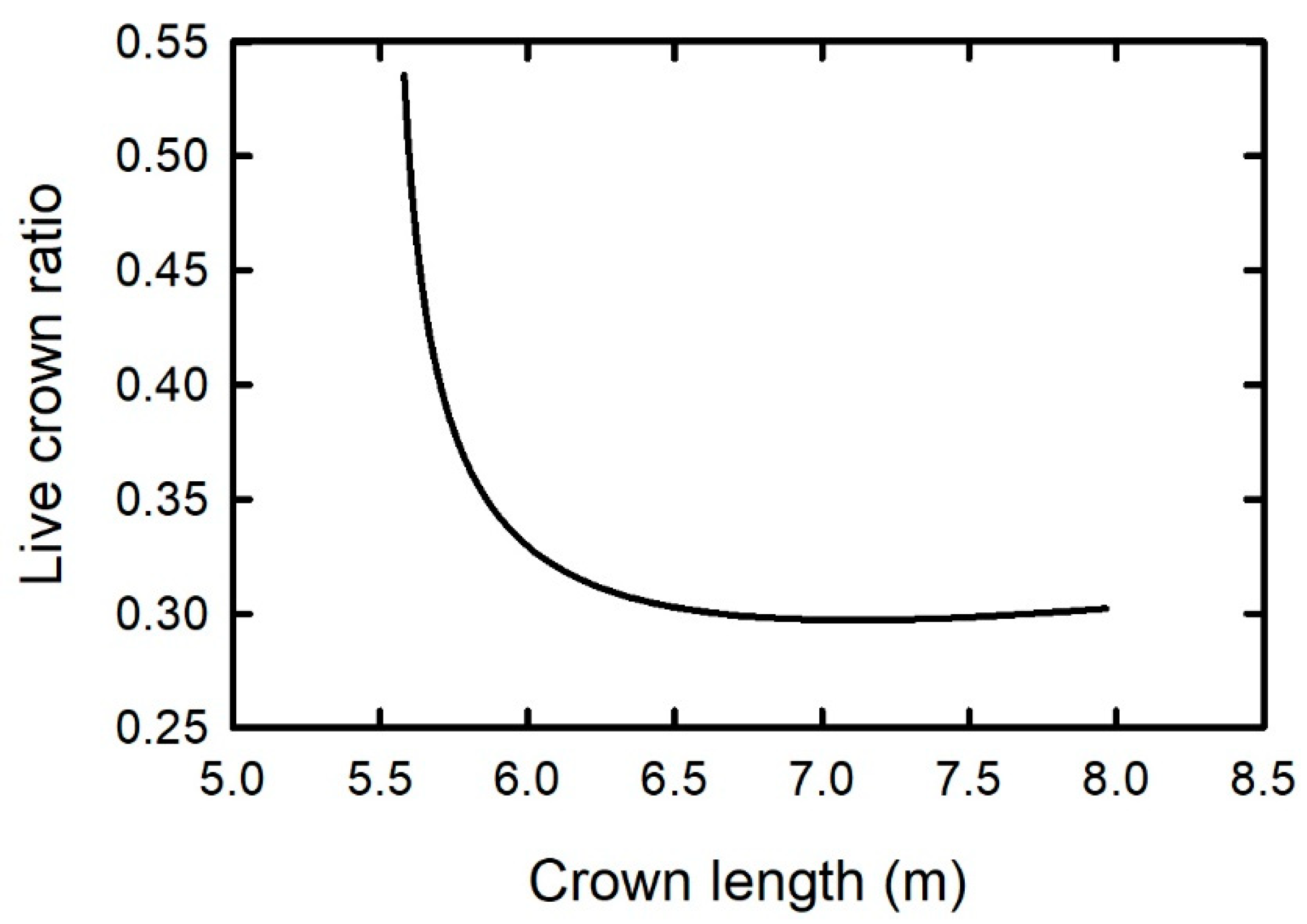
While the live-crown ratio is a function of live-crown length, the relationship between the two variables exhibits different phases depending on the stand’s stage of development, according to the biomechanical model of Dean et al. [15]. During the stand’s approach to self-thinning, the average live crown ratio decreases rapidly as the average live crown length increases (Figure 1). A minimum value of the live-crown ratio is reached sometime during self-thinning. The relationship changes at this point; the mean live-crown ratio becomes positively correlated with average live-crown, but with a slope just slightly greater than zero. This indicates, at least for loblolly pine, that the bottom of the live crown becomes somewhat fixed while crown length continues to increase with height growth. This same positive relationship between the live-crown ratio and crown length was observed by Dean and Long [44] in 80 and 120-year old lodgepole pine stands that were assumed to be self-thinning.
According to Smith [45] and Dean and Long [44], the relationship between the live-crown ratio is constant for an even-aged monoculture self-thinning at 100% relative density, i.e., traversing a straight line with a slope of −0.63 within a plane defined by the log of tree size vertically and the log of tree density horizontally. Neither the model output from the biomechanical model of Dean et al. [15] nor the data presented by Dean and Long [44] showed that the log of average stand diameter and the log of tree density formed a straight line; both were convex curves with respect to the origin. The purpose of the paper by Dean and Long [44] was to demonstrate the involvement of the uniform-stress principle of stem formation as an underlying mechanism for size-density relationships in even-aged monocultures. When Dean and Long [44] recalculated stem diameter setting the values of live-crown ratio to the overall average across the plots in their study, the plot of the resulting values of the log of average stand diameter and the log of tree density formed a straight line but with a significantly shallower slope. For the hypothetical loblolly pine plantation in Dean et al. [15], if the calculated values of the log of average stand diameter and the log of tree density calculated with the biomechanical model were linear, the corresponding plot between the live-crown ratio and crown length would presumably have a slope of zero.
The difficulty in elucidating the developmental profile of the live-crown ratio and crown depth is that data for these properties come from spacing studies. Consequently, the patterns formed in bivariate plots of these properties represent a slice through developmental stages; not a developmental trajectory through time. In the typical situation for southern pines, at least, where a stand grows to a size-density boundary, tracks it for a while (or not), then falls away (for example, [46,47]), stand density increases, remains constant temporarily, if at all, and then declines. Consequently, when a crown property canopy is plotted as a function of a competition index, the data are not necessarily in chronological order. Spacing studies attempt to compress time in order to develop predictive models, but they cannot fully account for developmental differences between young, pole-sized trees and mature saw timber-sized trees, both in the self-thinning stage. In addition, plots of mean size with tree density from spacing studies are more likely to display the competition-density effect described by Hutchings and Budd [48] instead of a true self-thinning trajectory that forms when mean size and tree are plotted for self-thinning stands of different ages. In order to ensure a complete analysis between the crown length and live-crown ratio, data need to be collected for spacing studies installed through time such that each developmental stage is represented across a range of ages.
2.2. Height to Median Leaf Area
The height to the median of the leaf area is a function of the vertical distribution of the leaf area. Below the live crown, this height remains constant. Consequently, the length of the lever arm (SH in Equation (1)) shortens as height H approaches the bottom of the crown. The solid created when only SH changes is a cubic paraboloid. This has been noted for several species, including [12,49] and [18] (p. 58). Within the live crown, both the leaf area above H (AH) and SH decrease simultaneously, resulting in a rapid decrease in stem diameter as H approaches the top of the crown. The geometry of the stem within the crown does not match a simple solid. The overall value of SH and its rate of change within the canopy, in addition to that of AH, are functions of the vertical distribution of leaf area.
The typical motivation for characterizing the vertical distribution of leaf area is its effect on light penetration through the canopy, and therefore, the distribution must be known in order to calculate the photosynthetic rate of the canopy in process models (e.g., [50]). Both destructive and in situ methods have been used to characterize the vertical distribution of foliage. In situ measurements use some form of a point quadrat, either a physical quadrat in the form of plumb bob or long needles moved down through the canopy, or a virtual one in the form of lasers or a periscope. Destructive measurements measure the foliage mass within fixed intervals within the crown and convert the biomass values to area with the specific leaf area for that interval. Destructive measurements allow only a single measurement in time, but the values are not inherently biased like estimates derived from point quadrats. The bias in point quadrat methods is due to the geometric interaction between the angle of the point quadrat and the leaf inclination angle. Wilson [51] produced a series of graphs displaying the effect of quadrat angle and leaf angle, showing that any systematic orientation of the leaves results in either a positive or negative bias in the estimate of foliage area, depending on the angle of the quadrat. The most negative bias occurs when the quadrat angle is parallel to the leaf angle, and the most positive bias occurs when the quadrat angle is perpendicular to the leaf angle. The bias can be minimized with two passes of the point quadrat through the canopy at two angles, which is never done. Destructive measurements can also be systematically biased if the height of the leaf area is set to the height to where the branch emerges from the stem [52]. Branches are generally curved upward at the top of the crown and are more horizontal toward the base of the crown. While this particular bias may affect light penetration into the crown, it does not affect the height to the median of the leaf area in calculating the length of the lever arm because from a mechanical perspective, the energy from wind pressure on the crown is transmitted to the stem where the branches attach to the stem.
When leaf area is expressed as relative leaf area in relation to relative height, the data can be described with probability density functions. Early analyses demonstrated the utility of describing foliage profiles with a normal distribution [53]. However, the normal distribution is too rigid to account for the skew of the foliage toward the bottom of the crown. Other distribution functions that can describe a wide variety of probability distributions have since been adapted to describe foliage profiles. The Weibull function can describe skewed distributions, and the parameters that shape the distribution can be regressed on factors that affect the distribution of leaf area. For instance, Schreuder and Swank [54] found that the Weibull distribution could be made to account for effects of site conditions such as site quality and stand density on the vertical profile of foliage. Xu and Harrington [55] regressed the shape and scale parameters for the Weibull function on the relative dominance of the tree and leaf area index of the stand (leaf area per unit ground area) to calculate the vertical distribution of foliage in loblolly pine plantations. Other probability density functions such as the beta distribution and the Johnson’s SB have proven useful in mathematically representing vertical foliage profiles.
Dean et al.’s [15] model uses the Johnson’s SB distribution for calculating the leaf area within the crown. The advantages of this distribution for calculating the vertical foliage profile are that the distribution is a function of the relative heights associated with the 15th and 50th percentiles of relative leaf area and that the starting and ending points for relative height are fixed at zero and one, with zero set to the top of the crown. The Weibull function starts at a relative height of zero but extends to infinity; the bottom of the crown has to be defined in terms of negligible changes in relative leaf area with a change in relative height. Jerez et al. [56] found that the relative height of the 15th and 50th percentiles of relative leaf area could be calculated with curvilinear functions of the live-crown ratio, total height, height to the crown midpoint, and tree age. The two models were fit with the seemingly unrelated regression procedure. The leaf above a given height and the height to median leaf area above that height were then calculated with the cumulative form of the Johnson’s SB probability density function.
The biomechanical model calculates the volume of the average tree in the stand and multiplies that value by the number of surviving trees in the stand to obtain stand values of volume and mean annual increment. Consequently, the equations for calculating the height to base of the crown and the vertical distribution of leaf area are assumed to represent the average tree in the stand. Dean and Long [44] found no discernable error between the observed quadratic mean diameter and the diameter calculated with mean leaf area per tree and the average height to the median of leaf area using the uniform-stress model for mature lodgepole pine in northern Utah. However, assuming that the vertical distribution of leaf area calculated for individual trees represents the leaf area of the average tree in the stand may be a source of significant error. Mori and Hagihara [57] characterized the vertical profiles of Chamaecyparis obtuse (Seib. et Zucc.) and found that foliage was distributed more normally in the taller trees and distributed closer to the top of smaller trees in the plantation. Jerez et al. [56] found that for individual trees, the bulk of the foliage moved from the bottom of the crown at young ages, to the top of the crown as the stands aged for loblolly pine. Maguire and Bennett [58] note that canopy profiles that developed from the crown profiles of individual trees in the stand share the most common distribution properties of the trees, but the aggregate profile has unique characteristics that do not exist in any particular tree. Consequently, reconstructing the composite distribution of foliage within a stand depends on the ability to accurately calculate the foliage distribution of every tree within the plot. Obviously, the ability to reconstruct the foliage distribution of a stand depends on adequate sampling of the constituents. For example, Xu and Harrington [55] only used one tree per plot to investigate the effect of cultural treatment on foliage profiles. They standardized the selected trees to a single crown position across the plots in order to test treatment effects, but the sampling design would be inadequate to make inferences about the treatment effects on the canopy as a whole.
Light detection and ranging (lidar) creates data for quantifying the vertical profile of canopy elements in three dimensions, eliminating the need to reconstruct the profile from individual trees. A complete description of lidar technology is available in Lefsky et al. [59]. To summarize simply, lidar is an active, remote-sensing technology for measuring distance. Laser pulses or beams are directed towards objects of interest, and the distance to the object is calculated from the return time of the reflected light. When directed downward from an aircraft toward a forest, the elevation where the laser was reflected from a surface in the forest is calculated from the distance the laser traveled and the height of the aircraft. This elevation or z value is combined with x and y coordinates (latitude and longitude) from a high-precision GPS unit within the instrument. Lidar platforms can be mounted in aircraft or on the ground. Either platform is suitable for characterizing the physical structure of forests stands as Zhao et al. [60] found good agreement between the airborne and ground-based profiles. Lidar systems have advanced rapidly, and lidar is becoming an accepted platform for remotely sensed forest inventory and ecological research [59,61,62,63,64].
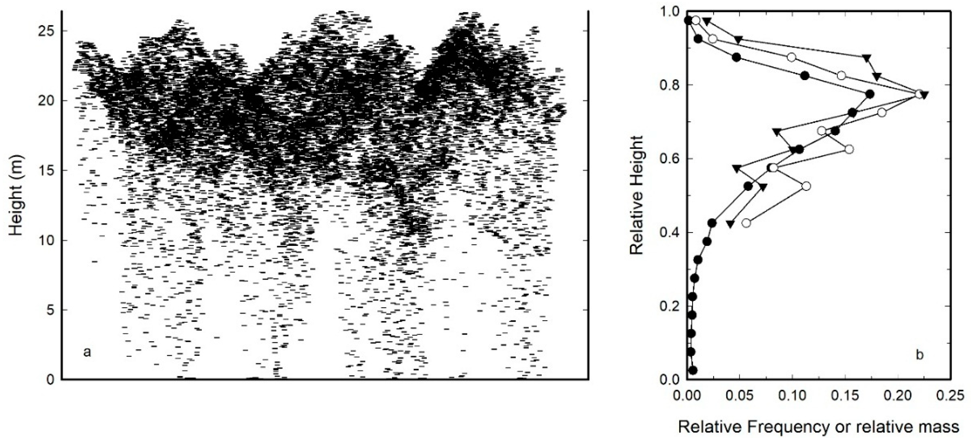
Within a specified horizontal boundary, the relative frequency of z values can be fit to probability density functions to quantitatively describe the vertical profile of reflections from the forest. The profile created from the lidar point cloud includes reflections from the stems, branches, and foliage (Figure 2a). Dean et al. [65] compared how well the height to the median leaf area could be estimated with airborne-based lidar and found no significant difference between ground-based and lidar-based measurements of the height to median leaf for an even-aged, 36-year-old loblolly pine stand (Figure 2b). In addition, Coops et al. [66] found satisfactory visual comparisons between the vertical distribution of lidar returns in a Douglas-fir—Hemlock forest and the interception of vertical point quadrats with foliage. Therefore, within the canopy, the foliage appears to cause the majority of the reflections; consequently, the median of the relative z values can be equated to the height to the median of the leaf area.
3. Mean Leaf Area per Tree
The amount of leaf area within a height interval within the crown is the product of the mean leaf area per tree and the relative leaf area. The most common method for estimating leaf area for a tree is with a formula built from ground-based measurements of tree dimensions. Sapwood cross-sectional area is the most logical predictor for leaf area per tree, being the conduit of water to the foliage, but for loblolly pine, Baldwin [68] found that DBH predicted leaf area per tree equally well. The biomechanical model calculates stem diameter as a function of leaf area; consequently, leaf area must be determined from the population effect on crown dimensions such as height to the top of the canopy and to the bottom of the canopy. The equation incorporated in the model was based on the regression model of Roberts et al. [69], with average tree height and height to the middle of the live crown (crown length divided by 2) as predictor variables. This model was developed with the intention of calculating the individual leaf area from LiDAR measured heights in loblolly pine plantations in order to test for treatment effects on LAI using remotely sensed data [70]. Other methods for estimating the leaf area index remotely have been proposed, such as regressing various statistical moments on ground-based measurements of the leaf area index or passive reflectance values [71] (p. 353).
Dean et al. [15] modified the leaf area equation of Roberts et al. [69] by replacing height to the middle of crown with live-crown length. According to the equation they used, average leaf area per tree increased exponentially with average tree height with the exponent equal to 4.03 and less steeply with live-crown length with the exponent equal to 1.42. Without mortality, the leaf area index is predicted to increase sharply with age on a site with average site quality and to begin to drop when self-thinning begins (Figure 3a). The sharp increase in the leaf area index predicted with the model agrees with data presented by King et al. [72] for a chronosequence of red pine (Pinus resinosa Ait.). They measured the allocation of carbon and nitrogen among the various aboveground components of the stand and found a sharp increase in the carbon allocated to the foliage with age. Carbon allocated to foliage in the oldest stand declined substantially, but unlike the younger stands, the oldest stand had been thinned. Carbon consistently comprises one half of the mass of foliage, so carbon is nearly a perfect surrogate for foliage mass. For the unthinned plots, total carbon in foliage rises just as quickly with age as the model values of the leaf area index do for loblolly pine (Figure 3b). Therefore, the steep increase in the leaf area index calculated with the biomechanical seems reasonable.
4. Potential for Including Physiological Processes in the Biomechanical Model
The biomechanical model of Dean et al. [15] is quite simple from a conceptual perspective. It calculates the profile of stem diameters necessary to counteract the bending stress generated along the tree stem from wind drag on the crown. What complicates the model is calculating the crown parameters responsible for the drag because the relationships between the height to the base of the live crown and the vertical distribution of leaf area as a function of population dynamics are only available from purely statistical fits of models to data. The regular relationships between crown length and tree spacing and between the live-crown ratio with combinations of tree size and tree density would seem to suggest an underlying, evolutionary basis for the spacing of foliage that could eventually replace empirical equations in the biomechanical model with more process-based equations. Many studies have been conducted to characterize foliage display in both temporal and spatial terms in order to better understand the variables influencing stand production [73,74,75,76]. Other than Sprugel’s [77] comparison of the costs and benefits of foliage display between needle-bearing and broadleaf-bearing species, no other analysis has attempted to relate branch and foliage arrangement to production ecology from an evolutionary perspective.
Another important aspect of the biomechanical model of Dean et al. [15] is height growth, in that it serves to establish the top of the crown. While tree density affects the height to the bottom of the crown, height changes independently of tree density, with the exception of exceptionally high or low densities. Since leaf area per tree is also a function of the height to the bottom of the crown, height increment adds to leaf area while competition reduces it. Height increases rapidly with age during the juvenile stage, towards an asymptotic value at old age. It is for this reason that crown length increases rapidly while the stand is young, until reaching a somewhat stable or slowly changing value during the self-thinning stage on to old growth. The more protracted the juvenile of height growth, the more leaf area that will accumulate on the average tree in the stand, resulting in larger stem diameters. This is often the dimensional response to nutrient amendments [78,79,80,81]. Nutrient amendments may also increase competition among the trees compared to a paired, untreated stand, resulting in greater heights to the base of the live crown, but the increase is not enough to offset the effect of increased height on average leaf area and the resultant increase in average diameter.
Height in growth and yield models is calculated with age and site index (the height of the tallest trees most reflective of site productivity at a specified age). The emphasis given to formulating height equations in growth and yield models has been on the accuracy and precision of the estimate (for example, [82,83]). Statistical approaches are best when accuracy and precision are the goals, but they do little to further the understanding of the physiological factors that determine how fast the terminal leader will grow during a season. Some aspects of leader extension have been investigated but no synthesis has attempted to combine the morphological development of leader extension, growth hormones, and physiology with the physical environment to simulate height growth over time. Regression models have been constructed to estimate the site index from soil and climate variables (e.g., [84]), but site index does not relate directly to height at any age. A process-based model for height increment would make a significant contribution to understanding and simulating forest stand production.
5. Conclusions
Unless a tree is damaged, the size of a tree’s crown determines the size of its stem. Production ecologists and quantitative silviculturists in particular have refined this association to the point where resource professionals can calculate, with some degree of confidence, the change in production expected by managing density effects on crown size [10]. Dean [85] makes the connection between crown and stem dimensions with the uniform-stress model and has demonstrated how much stem growth could be expected with given changes in the amount and distribution of foliage in the crown. He even showed how this coordinated morphology could account for changes in leaf area efficiency with increasing stand occupancy. Dean and Baldwin [86] also demonstrated how crown characteristics through the uniform-stress principle determined the values of Reineke’s stand density index, a common measure of stand density and competition.
Jaffe [87] coined the term thigmomorphogenisis to describe the response of plants to wind. In trees, mechanical stimulation of the stems will increase their elasticity, requiring a larger cross section to maintain stiffness [21,88]. Trees will also slow height growth when exposed to wind [88,89]. Lundqvist and Elfin [90] worked with a Scot’s pine (Pinus sylvestris L.) plantation where the trees had been planted using a repeated pattern of various spacings, thus creating a range of repeated spacings within the stand. They analyzed the conformance of the tree morphology to the uniform-stress principles for a sampling of repeated spacing units. They reasoned that the trees with larger gaps between neighbors would encounter higher wind velocities than trees with narrower gaps; consequently, the trees with wider spacings would have larger stem diameters than trees with narrower spacings for the same combination of leaf area and height to the median of leaf area. They failed to reject that hypothesis and concluded that spacing had no effect on the fit of the uniform-stress hypothesis to the data collected from these trees. Dean and Long [16] did not detect any effect of canopy position in the fit of the uniform-stress model to the data they collected from lodgepole pine stands. Such findings seem to suggest that under normal wind climates, trees in a stand have a common set point that coordinates stem size and crown dimensions.
Studies have demonstrated that stem diameter can be predicted with existing crown dimensions. The biomechanical model of Dean et al. [15] aids in furthering our understanding of how crown size is related to stem geometry. It specifically addresses the question “is our current understanding of competition effects on crown dynamics sufficient to accurately predict stem geometry?” Studies indicate that variables such as crown length and the live-crown ratio are related to stand spacing and competition, but the relationships are imprecise due to mechanical abrasion between the crowns that create gaps in the canopy. Crown shyness, as this is called, allows more light to penetrate than would be expected with complete canopy coverage, adding imprecision to the relationship. Crown shyness also adds variation to relationships between the live-crown ratio and stand density. The vertical profile of foliage is also affected by crown shyness, but the largest contributor to uncertainty in quantifying the relative distribution of foliage within a crown is tree-to-tree variation in the distribution. The vertical profile of foliage in the canopy is best described from a section of the canopy, not from the individual trees that comprise that section. Lidar has promise in characterizing the vertical profile of foliage within a given section of the canopy. Average leaf area is a difficult parameter to estimate with the biomechanical model because the model calculates stem diameter from crown properties; leaf area is usually calculated from stem dimensions. For the biomechanical model, leaf area is calculated from tree height and crown length, with height making a much larger contribution to the calculation than crown length. Tree height is the one variable in the model affecting the average stem diameter that is not related to stand density. The systematic relationships between crown properties and competition between neighboring trees may help advance the understanding of the physiological underpinnings of these relationships, enabling these statistical relationships to be replaced with more process-based formulae.
Funding
This research was supported in part by the National Institute of Food and Agriculture, McIntire Stennis Project LAB94307. LiDAR data and analyses was supported with funds from a cooperative agreement with the US Forest Service, Southern Research Station (SRS 01-CA-11330122-510), Louisiana Department of Agriculture and Forestry’s Louisiana Forest Productivity Program (CFMS #577795/Proj #01-FPP1), and the Mississippi State University’s Remote Sensing Technology Center.
Acknowledgments
Published with the approval of the Director of the Louisiana Agricultural Experiment Station as publication No. 2018-241-32175.
Conflicts of Interest
I declare no conflict of interest.
References
- Comstock, J.P.; Sperry, J.S. Theoretical considerations of optimal conduit length for water transport in vascular plants. New Phytol. 2000, 148, 195–218. [Google Scholar] [CrossRef]
- Sperry, J.S. Coordinating stomatal and xylem functioning—An evolutionary perspective. New Phytol. 2004, 162, 568–570. [Google Scholar] [CrossRef]
- Gardiner, B.; Byrne, K.; Hale, S.; Kamimura, K.; Mitchell, S.J.; Peltola, H.; Ruel, J.-C. A review of mechanistic modelling of wind damage risk to forests. Forestry 2008, 81, 447–463. [Google Scholar] [CrossRef] [Green Version]
- Moulia, B.; Coutand, C.; Julien, J.-L. Mechanosensitive control of plant growth: Bearing the load, sensing, transducing, and responding. Front. Plant Sci. 2015, 6, 52. [Google Scholar] [CrossRef] [PubMed]
- Valentine, H.T.; Amateis, R.L.; Gove, J.H.; Makela, A. Crown-rise and crown-length dynamics: Application to loblolly pine. Forestry 2013, 86, 371–375. [Google Scholar] [CrossRef]
- Mar:Möller, C. The effects of thinning, age, and site on foliage, increment, and loss of dry matter. J. For. 1947, 45, 393–404. [Google Scholar] [CrossRef]
- Madgwick, H.A.I.; Olson, D.F. Leaf area index and volume growth in thinned stands of Liriodendron tulipifera L. J. Appl. Ecol. 1974, 11, 575–579. [Google Scholar] [CrossRef]
- Martin, T.A.; Jokela, E.J. Stand development and production dynamics of loblolly pine under a range of cultural treatments in north-central Florida USA. For. Ecol. Manag. 2004, 192, 39–58. [Google Scholar] [CrossRef]
- Long, J.N.; Dean, T.J.; Roberts, S.D. Linkages between silviculture and ecology: Examination of several important conceptual models. For. Ecol. Manag. 2004, 200, 249–261. [Google Scholar] [CrossRef]
- Dean, T.J.; Baldwin, V.C. Crown management and stand density. In Growing Trees in a Greener World: Industrial Forestry in the 21st Century; 35th LSU Forestry Symposium; Carter, M.C., Ed.; Louisiana State University Agricultural Center, Louisiana Agricultural Experiment Station: Baton Rouge, LA, USA, 1996; pp. 148–159. [Google Scholar]
- Whitehead, D.; Edwards, W.R.N.; Jarvis, P.G. Conducting sapwood area, foliage area, and permeability in mature trees of Piceasitchensis and Pinuscontorta. Can. J. For. Res. 1984, 14, 940–947. [Google Scholar] [CrossRef]
- Long, J.N.; Smith, F.W.; Scott, D.R.W. The role of Douglas-fir stem sapwood and heartwood in the mechanical and physiological support of crown and development of stem form. Can. J. For. Res. 1981, 11, 459–464. [Google Scholar] [CrossRef]
- Mencuccini, M.; Grace, J.; Fioravanti, M. Biomechanical and hydraulic determinants of tree structure in Scots pine: Anatomical characteristics. Tree Physiol. 1997, 17, 105–113. [Google Scholar] [CrossRef] [PubMed]
- Woodrum, C.L.; Ewers, F.W.; Telewski, F.W. Hydraulic, biomechanical, and anatomical interactions of xylem from five species of Acer (Aceraceae). Am. J. Bot. 2003, 90, 693–699. [Google Scholar] [CrossRef] [PubMed] [Green Version]
- Dean, T.J.; Jerez, M.; Cao, Q.V. A simple stand growth model based on canopy dynamics and biomechanics. For. Sci. 2013, 59, 335–344. [Google Scholar] [CrossRef]
- Dean, T.J.; Long, J.N. Validity of constant-stress and elastic instability principles of stem formation in Pinus contorta and Trifolium pratense. Ann. Bot. 1986, 54, 833–840. [Google Scholar] [CrossRef]
- Metzger, K. Der Wind als massgebender Faktor für das Wachtsum der Bäume. Mundener Forstl. Hefte 1893, 3, 35–86. [Google Scholar]
- Assmann, E. The Principles of Forest Yield Study; Pergamon Press, Inc.: New York, NY, USA, 1970. [Google Scholar]
- Jokela, E.J.; Harding, R.B.; Nowak, C.A. Long-term effects of fertilization on stem form, growth relations, and yield estimates of slash pine. For. Sci. 1989, 35, 832–842. [Google Scholar] [CrossRef]
- Morgan, J.; Cannell, M.G.R. Shape of tree stems—A re-examination of the uniform stress hypothesis. Tree Physiol. 1994, 14, 49–62. [Google Scholar] [CrossRef] [PubMed]
- Dean, T.J.; Roberts, S.D.; Gilmore, D.W.; Maguire, D.A.; Long, J.N.; O’Hara, K.L.; Seymour, R.S. An evaluation of the uniform stress hypothesis based on stem geometry in selected North American conifers. Trees Struct. Funct. 2002, 16, 559–568. [Google Scholar] [CrossRef]
- Cao, Q.V.; Dean, T.J. Predicting diameter at breast height from total height and crown length. In Proceedings of the 15th Bennial Southern Silvicultural Research Conference, SRS-GTR-17; Guldin, J.M., Ed.; U.S. Department of Agriculture, Forest Service, Southern Research Station: Asheville, NC, USA, 2013; pp. 201–205. [Google Scholar]
- Kidombo, S.D.; Dean, T.J. Growth of tree diameter and stem taper as affected by reduced leaf area on selected branch whorls. Can. J. For. Res. 2018, 48, 317–323. [Google Scholar] [CrossRef]
- West, P.W.; Jackett, D.R.; Sykes, S.J. Stresses in, and the shape of, tree stems in forest monoculture. J. Theor. Biol. 1989, 140, 327–343. [Google Scholar] [CrossRef]
- Niklas, K.J.; Spatz, H.C. Wind-induced stresses in cherry trees: Evidence against the hypothesis of constant stress levels. Trees Struct. Funct. 2000, 14, 230–237. [Google Scholar] [CrossRef]
- Minamino, R.; Tateno, M. Variation in susceptibility to wind along the trunk of an isolated Larix kaempferi (Pinaceae) tree. Am. J. Bot. 2014, 101, 1085–1091. [Google Scholar] [CrossRef] [PubMed]
- Dean, T.J. Effect of growth rate and wind sway on the relation between mechanical and water-flow properties in slash pine seedlings. Can. J. For. Res. 1991, 21, 1501–1506. [Google Scholar] [CrossRef]
- Valinger, E.; Lundqvist, L.; Sundberg, B. Mechanical stress during dormancy stimulates stem growth of scots pine seedlings. For. Ecol. Manag. 1994, 67, 299–303. [Google Scholar] [CrossRef]
- Lundqvist, L.; Valinger, E. Stem diameter growth of scots pine trees after increased mechanical load in the crown during dormancy and (or) growth. Ann. Bot. 1996, 77, 59–62. [Google Scholar] [CrossRef]
- Valentine, H.T.; Ludlow, A.R.; Furnival, G.M. Modeling crown rise in even-aged stands of Sitka spruce or loblolly pine. For. Ecol. Manag. 1994, 69, 189–197. [Google Scholar] [CrossRef]
- Long, J.N. A pratical approach to density management. For. Chron. 1985, 61, 23–27. [Google Scholar] [CrossRef]
- Dean, T.J.; Baldwin, V.C., Jr. Growth in loblolly pine plantations as a function of stand density and canopy properties. For. Ecol. Manag. 1996, 82, 49–58. [Google Scholar] [CrossRef]
- Beekhuis, J. Crown depth of radiata pine in relation to stand density and height. N. Z. J. For. 1965, 10, 43–61. [Google Scholar]
- Meng, S.X.; Rudnicki, M.; Lieffers, V.J.; Reid, D.E.B.; Silins, U. Preventing crown collisions increases the crown cover and leaf area of maturing lodgepole pine. J. Ecol. 2006, 94, 681–686. [Google Scholar] [CrossRef] [Green Version]
- Long, J.N.; Smith, F.W. Volume increment in Pinus contorta var. latifolia: The influence of stand development and crown dynamics. For. Ecol. Manag. 1992, 53, 53–64. [Google Scholar] [CrossRef]
- Putz, F.E. Mechanical abrasion and intercrown spacing. Am. Midl. Nat. 1984, 112, 24–28. [Google Scholar] [CrossRef]
- Ward, W.W. Live Crown Ratio and Stand Density in Young, Even-Aged, Red Oak Stands. For. Sci. 1964, 10, 56–65. [Google Scholar] [CrossRef]
- Dyer, M.E.; Burkhart, H.E. Compatible crown ratio and crown height models. Can. J. For. Res. 1987, 17, 572–574. [Google Scholar] [CrossRef]
- Hasenauer, H.; Monserud, R.A. A crown ratio model for Austrian forests. For. Ecol. Manag. 1996, 84, 49–60. [Google Scholar] [CrossRef]
- Dean, T.J. Using live-crown ratio to control wood quality: An example of quantitative silviculture. Presented at the Tenth Bennial Southern Silvicultural Research Conference, Shreveport, LA, USA, 16 February 1999; Haywood, J.D., Ed.; Gen. Tech. Rep. SRS-30. U.S. Department of Agriculture, Southern Research Station: Asheville, NC, USA, 1999; pp. 511–514. [Google Scholar]
- Zhao, D.; Kane, M.; Borders, B.E. Crown ratio and relative spacing relationships for Loblolly pine plantations. Open J. For. 2012, 2, 110–115. [Google Scholar] [CrossRef]
- Wilson, F.G. Numerical expression of stocking in terms of height. J. For. 1946, 44, 758–761. [Google Scholar]
- Hasenauer, H.; Monserud, R.A.; Gregoire, T.G. Using simultaneous regression techniques with individual-tree growth models. For. Sci. 1998, 44, 87–95. [Google Scholar] [CrossRef]
- Dean, T.J.; Long, J.N. Influence of leaf area and canopy structure on size-density relations in even-aged lodgepole pine stands. For. Ecol. Manag. 1992, 49, 109–117. [Google Scholar] [CrossRef]
- Smith, N.J. A model of stand allometry and biomass allocation during the self-thinning process. Can. J. For. Res. 1986, 16, 990–995. [Google Scholar] [CrossRef]
- Cao, Q.V.; Dean, T.J.; Baldwin, V.C., Jr. Modeling the size-density relationship in direct-seeded slash pine stands. For. Sci. 2000, 46, 317–324. [Google Scholar] [CrossRef]
- VanderSchaaf, C.L. Estimating individual stand size-density trajectories and a maximum size-density relationship species boundary line slope. For. Sci. 2010, 56, 327–335. [Google Scholar] [CrossRef]
- Hutchings, M.J.; Budd, C.S.J. Plant competition and its course through time. Bioscience 1981, 3, 640–645. [Google Scholar] [CrossRef]
- Gray, H.R. The Form and Taper of Forest-Tree Stems; Imperian Forestry Institute, University of Oxford: Oxford, UK, 1956. [Google Scholar]
- Wang, Y.P.; Jarvis, P.G. Influence of crown structural properties on PAR absorption, photosynthesis, and transpiration in sitka spruce—Application of a model (MAESTRO). Tree Physiol. 1990, 7, 297–316. [Google Scholar] [CrossRef] [PubMed]
- Wilson, J.W. Estimation of foliage denseness and foliage angle by inclined point quadrats. Aust. J. Bot. 1963, 11, 95–105. [Google Scholar] [CrossRef]
- Stenberg, P.; Kuuluvainen, T.; Kellomäki, S.; Jokela, E.J.; Gholz, H.L.; Gholz, H.L.; Linder, S.; McMurtrie, R.E. Crown structure, light interception, and productivity of pine trees and stands. Ecol. Bull. 1994, 43, 20–34. [Google Scholar]
- Stephens, G.R. Productivity of red pine, 1. Foliage distribution in tree crown and stand canopy. Agric. Meteorol. 1969, 6, 275–282. [Google Scholar] [CrossRef]
- Schreuder, H.T.; Swank, W.T. Coniferous Stands Characterized with The Weibull Distribution. Can. J. For. Res. 1974, 4, 518–523. [Google Scholar] [CrossRef]
- Xu, M.; Harrington, T.B.; Edwards, M.B. Responses of Loblolly Pine Biomass and Specific Leaf Area to Various Site Preparation Treatments; Edwards, M.B., Ed.; U.S.D.A., Forest Service, Southern Research Station: Ashsville, NC, USA, 1995; pp. 495–499.
- Jerez, M.; Dean, T.J.; Cao, Q.V.; Roberts, S.D. Describing leaf area distribution in loblolly pine trees with Johnson’s SB function. For. Sci. 2005, 51, 93–101. [Google Scholar] [CrossRef]
- Mori, S.; Hagihara, A. Crown profile of foliage area characterized with the weibull distribution in a hinoki (Chamaecyparis obtusa) stand. Trees Struct. Funct. 1991, 5, 149–152. [Google Scholar] [CrossRef]
- Maguire, D.A.; Bennett, W.S. Patterns in vertical distribution of foliage in young coastal Douglas-fir. Can. J. For. Res. 1996, 26, 1991–2005. [Google Scholar] [CrossRef]
- Lefsky, M.A.; Cohen, W.B.; Parker, G.G.; Harding, D.J. Lidar remote sensing for ecosystem studies. Bioscience 2002, 52, 19–30. [Google Scholar] [CrossRef]
- Zhao, F.; Yang, X.; Strahler, A.H.; Schaaf, C.L.; Yao, T.; Wang, Z.; Román, M.O.; Woodcock, C.E.; Ni-Meister, W.; Jupp, D.L.B.; et al. A comparison of foliage profiles in the Sierra National Forest obtained with a full-waveform under-canopy EVI lidar system with the foliage profiles obtained with an airborne full-waveform LVIS lidar system. Remote Sens. Environ. 2013, 136, 330–341. [Google Scholar] [CrossRef]
- Lim, K.; Treitz, P.; Wulder, M.; St-Onge, B.; Flood, M. Lidar Remote Sensing of Forest Structure. Prog. Phys. Geogr. 2003, 27, 88–106. [Google Scholar] [CrossRef]
- Parker, R.C.; Evans, D.L. An Application of Lidar in a Double-Sample Forest Inventory. West. J. Appl. For. 2004, 19, 95–101. [Google Scholar] [CrossRef]
- Evans, D.L.; Roberts, S.D.; Parker, R.C. LiDAR—A new tool for forest measurements? For. Chron. 2006, 82, 211–218. [Google Scholar] [CrossRef]
- Hyyppä, J.; Hyyppä, H.; Leckie, D.; Gougeon, F.; Yu, X.; Maltamo, M. Review of methods of small-footprint airborne laser scanning for extracting forest inventory data in boreal forests. Int. J. Remote Sens. 2008, 29, 1339–1366. [Google Scholar] [CrossRef]
- Dean, T.J.; Cao, Q.V.; Roberts, S.D.; Evans, D.L. Measuring heights to crown base and crown median with LiDAR in a mature, even-aged loblolly pine stand. For. Ecol. Manag. 2009, 257. [Google Scholar] [CrossRef]
- Coops, N.C.; Hilker, T.; Wulder, M.A.; St-Onge, B.; Newnham, G.; Siggins, A.; Trofymow, J.A.T. Estimating canopy structure of Douglas-fir stands from discrete-return LiDAR. Trees Struct. Funct. 2007, 21, 295–310. [Google Scholar] [CrossRef]
- Cao, Q.V.; Dean, T.J. Modeling crown structure from LiDAR data with statistical distributions. For. Sci. 2011, 57, 359–364. [Google Scholar]
- Baldwin, J.V.C. Is sapwood area a better predictor of loblolly pine crown biomass than bole diameter. Biomass 1989, 20, 177–185. [Google Scholar] [CrossRef]
- Roberts, S.D.; Dean, T.J.; Evans, D.L. Family influences on leaf area estimates derived from crown and tree dimensions in Pinus taeda. For. Ecol. Manag. 2003, 172, 261–270. [Google Scholar] [CrossRef]
- Roberts, S.D.; Dean, T.J.; Evans, D.L.; McCombs, J.W.; Harrington, R.L.; Glass, P.A. Estimating individual tree leaf area in loblolly pine plantations using LiDAR-derived measurements of height and crown dimensions. For. Ecol. Manag. 2005, 213, 54–70. [Google Scholar] [CrossRef]
- Fang, H.; Xiao, Z.; Qu, Y.; Song, J. Leaf Area Index. In Advanced Remote Sensing; Liang, S., Li, X., Wang, J., Eds.; Academic Press: San Diego, CA, USA, 2012; pp. 347–381. ISBN 9780123859549. [Google Scholar]
- King, J.S.; Giardina, C.P.; Pregitzer, K.S.; Friend, A.L. Biomass partitioning in red pine (Pinus resinos) along a chronosequence in the Upper Peninsula of Michigan. Can. J. For. Res. 2007, 37, 93–102. [Google Scholar] [CrossRef]
- Gillespie, A.; Allen, H.; Vose, J.M. Amount and vertical distribution of foliage of young loblolly pine trees as affected by canopy position and silvicultural treatment. Can. J. For. Res. 1994, 24, 1337–1344. [Google Scholar] [CrossRef]
- Pearcy, R.W.; Yang, W.M. A three-dimensional crown architecture model for assessment of light capture and carbon gain by understory plants. Oecologia 1996, 108, 1–12. [Google Scholar] [CrossRef] [PubMed]
- Albaugh, T.J.; Allen, H.L.; Fox, T.R. Individual tree crown and stand development in Pinus taeda under different fertilization and irrigation regimes. For. Ecol. Manag. 2006, 234, 10–23. [Google Scholar] [CrossRef]
- Kennedy, M. Functional–structural models optimize the placement of foliage units for multiple whole-canopy functions. Ecol. Res. 2010, 25, 723–732. [Google Scholar] [CrossRef]
- Sprugel, D.G. The relationship of evergreenness, crown architecture, and leaf size. Am. Nat. 1989, 133, 465–479. [Google Scholar] [CrossRef]
- Brix, H. Effects of thinning and nitrogen fertilization on growth of Douglas-fir: Relative contribution of foliage quantity and efficiency. Can. J. For. Res. 1983, 13, 167–175. [Google Scholar] [CrossRef]
- Teskey, R.O.; Gholz, H.L.; Cropper, W.P. Influence of climate and fertilization on net photosynthesis of mature slash pine. Tree Physiol. 1994, 14, 1215–1227. [Google Scholar] [CrossRef] [PubMed]
- Albaugh, T.J.; Allen, H.L.; Dougherty, P.M.; Kress, L.W.; King, J.S. Leaf area and above- and belowground growth responses of loblolly pine to nutrient and water additions. For. Sci. 1998, 44, 317–328. [Google Scholar]
- Jokela, E.J.; Dougherty, P.M.; Martin, T.A. Production dynamics of intensively managed loblolly pine stands in the southern United States: A synthesis of seven long-term experiments. For. Ecol. Manag. 2004, 192, 117–130. [Google Scholar] [CrossRef]
- Cieszewski, C.; Bailey, R.L. Generalized algebraic difference approach: Theory based derivation of dynamic site equations with polymorphism and variable asymptotes. For. Sci. 2000, 46, 116–126. [Google Scholar]
- Cieszewski, C.J. Three methods of deriving advanced dynamic site equations demonstrated on inland Douglas-fir site curves. Can. J. For. Res. 2001, 31, 165–173. [Google Scholar] [CrossRef]
- Gömöryova, E.; Gömory, D. Relationships between environmental factors and height growth and yield of Norway spruce stands: A factor-analytic approach. Forestry 1995, 68, 145–152. [Google Scholar] [CrossRef]
- Dean, T.J. Basal area increment and growth efficiency as functions of canopy dynamics and stem mechanics. For. Sci. 2004, 50, 106–116. [Google Scholar]
- Dean, T.J.; Baldwin, V.C., Jr. The relationship between Reineke’s stand-density index and physical stem mechanics. For. Ecol. Manag. 1996, 81, 25–34. [Google Scholar] [CrossRef]
- Jaffe, M.J. Thigmomorphogenesis: The response of plant growth and development to mechanical stimulation. Planta 1973, 114, 143–157. [Google Scholar] [CrossRef] [PubMed]
- Telewski, F.W.; Jaffe, M. Thigmomorphogenesis: Anatomical, morphological and mechanical analysis of genetically different sibs of Pinus taeda in response to mechanical pertubation. Physiol. Plant. 1986, 66, 219–226. [Google Scholar] [CrossRef] [PubMed]
- Telewski, F.W.; Pruyn, M.L. Thigmomorphogenesis: A dose response to flexing in Ulmus americana seedlings. Tree Physiol. 1998, 18, 65–68. [Google Scholar] [CrossRef] [PubMed]
- Lundqvist, L.; Elfving, B. Influence of biomechanics and growing space on tree growth in young Pinus sylvestris stands. For. Ecol. Manag. 2010, 260, 2143–2147. [Google Scholar] [CrossRef]
Figure 1.
Hypothetical relationship between average live-crown ratio and average live-crown length for a loblolly pine plantation from 10 to 50-years old calculated with the biomechanical model of Dean et al. (2013). Initial planting density = 1200 trees/ha and site index = 18 m at base age = 25 years.

Figure 2.
Section view of LiDAR elevation values from a 25 m × 25 m plot in a 36-year-old loblolly pine stand in southeastern Louisiana (a) and the distribution of elevation values (closed circles) overlain on the measured distribution of crown mass (branch plus foliage) (open circles) and foliage mass (closed triangles) for the same plot (b). Data in (a) collected with an Optech ALTM-1225 laser mapping system operating at 25 kHz and a scanning angle of ±9°. Analysis in (b) based on Cao and Dean [67].

Figure 3.
Comparison of accumulated leaf area calculated from the biomechanical model of Dean et al. [15] for a loblolly pine plantation started at 1200 trees/ha on land with site index = 18 m at 25 years (a) and measured accumulation of carbon in leaf mass for a chronosequence of a red pine plantation as reported by King et al. [72] (b) with an average tree density of 1750 trees/ha. The oldest red pine stand had been thinned to 622 trees/ha.

© 2018 by the author. Licensee MDPI, Basel, Switzerland. This article is an open access article distributed under the terms and conditions of the Creative Commons Attribution (CC BY) license (http://creativecommons.org/licenses/by/4.0/).
Share and Cite
MDPI and ACS Style
Dean, T.J. Neighbor and Height Effects on Crown Properties Associated with the Uniform-Stress Principle of Stem Formation. Forests 2018, 9, 334. https://doi.org/10.3390/f9060334
AMA Style
Dean TJ. Neighbor and Height Effects on Crown Properties Associated with the Uniform-Stress Principle of Stem Formation. Forests. 2018; 9(6):334. https://doi.org/10.3390/f9060334
Chicago/Turabian StyleDean, Thomas J. 2018. "Neighbor and Height Effects on Crown Properties Associated with the Uniform-Stress Principle of Stem Formation" Forests 9, no. 6: 334. https://doi.org/10.3390/f9060334
Note that from the first issue of 2016, this journal uses article numbers instead of page numbers. See further details here.