Machine Learning Approaches for Estimating Forest Stand Height Using Plot-Based Observations and Airborne LiDAR Data


Abstract
:
1. Introduction
2. Data and Methods
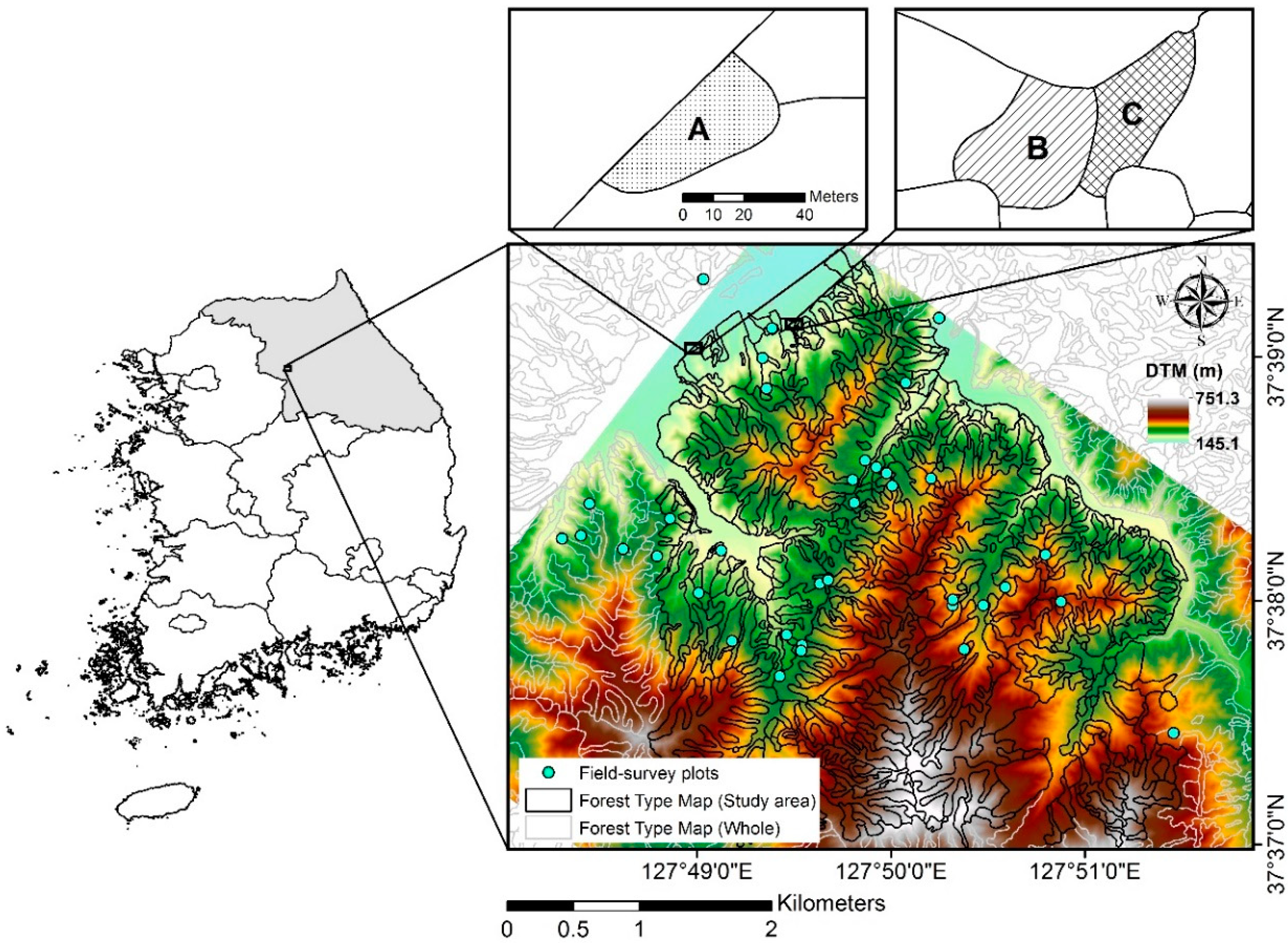
2.1. Study Area
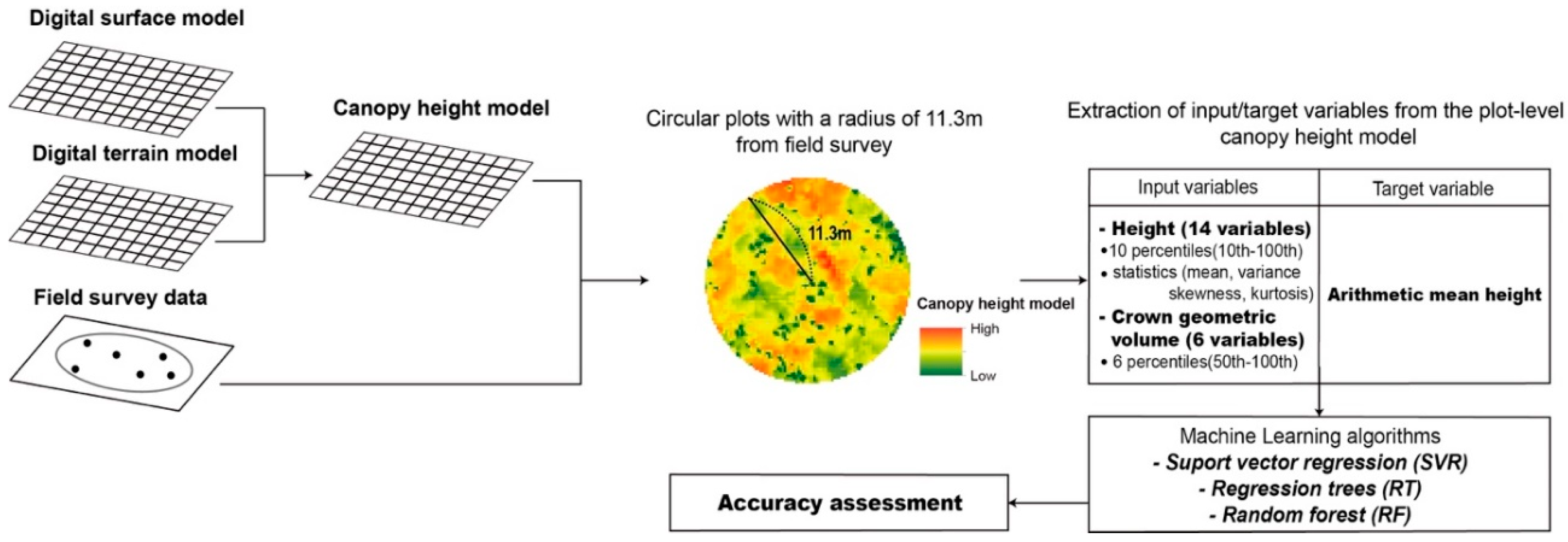
2.2. Data
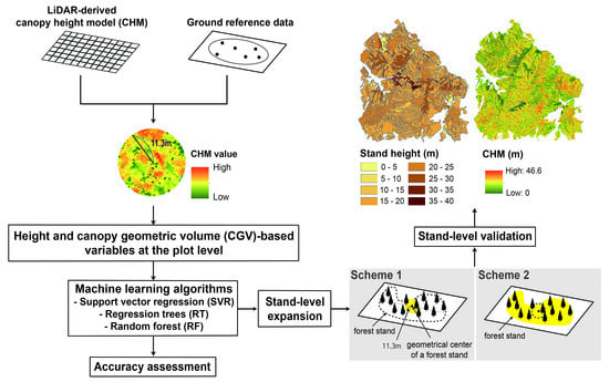
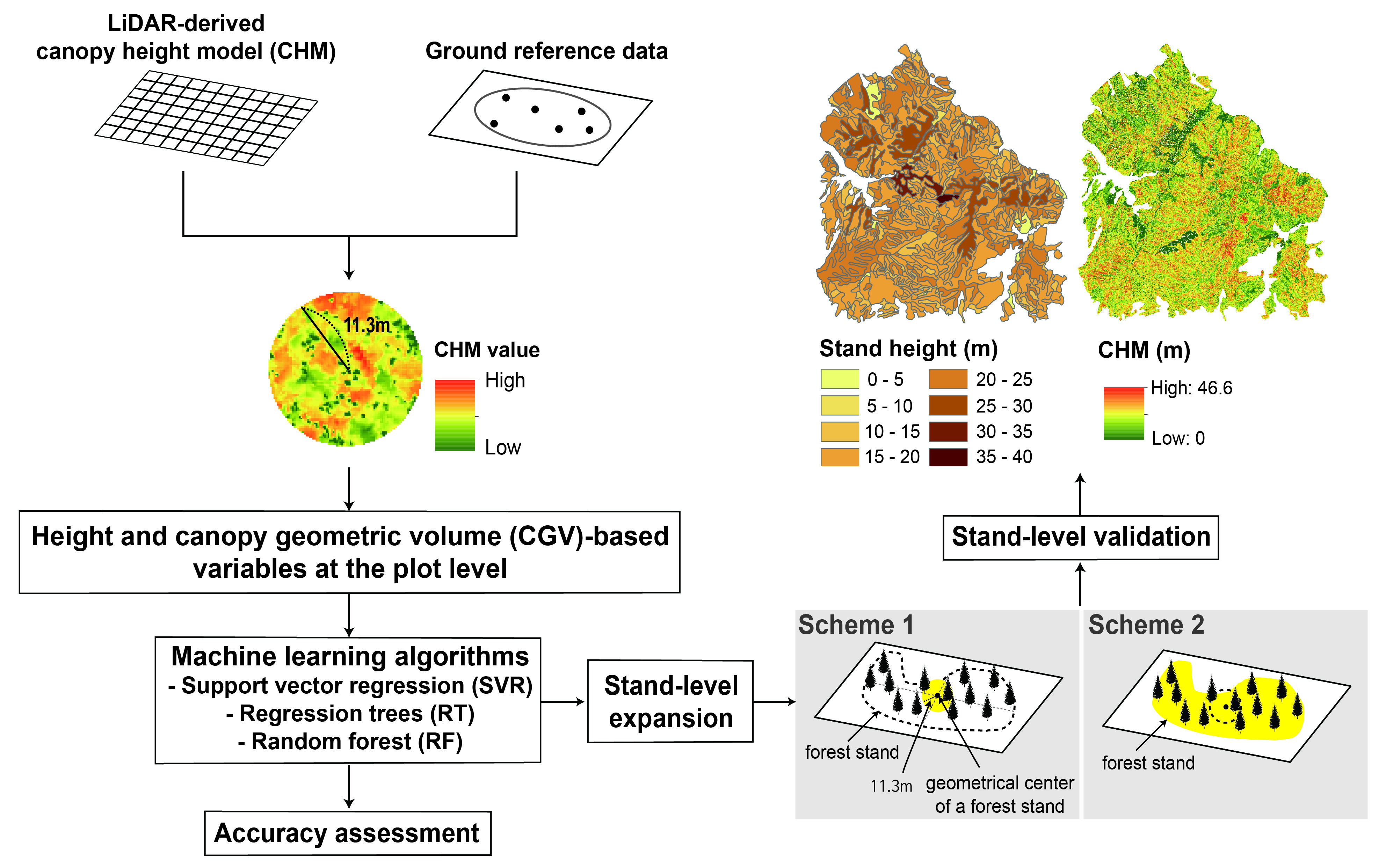
2.3. Methods
3. Results and Discussion
3.1. Comparison of Plot-Level Height Models
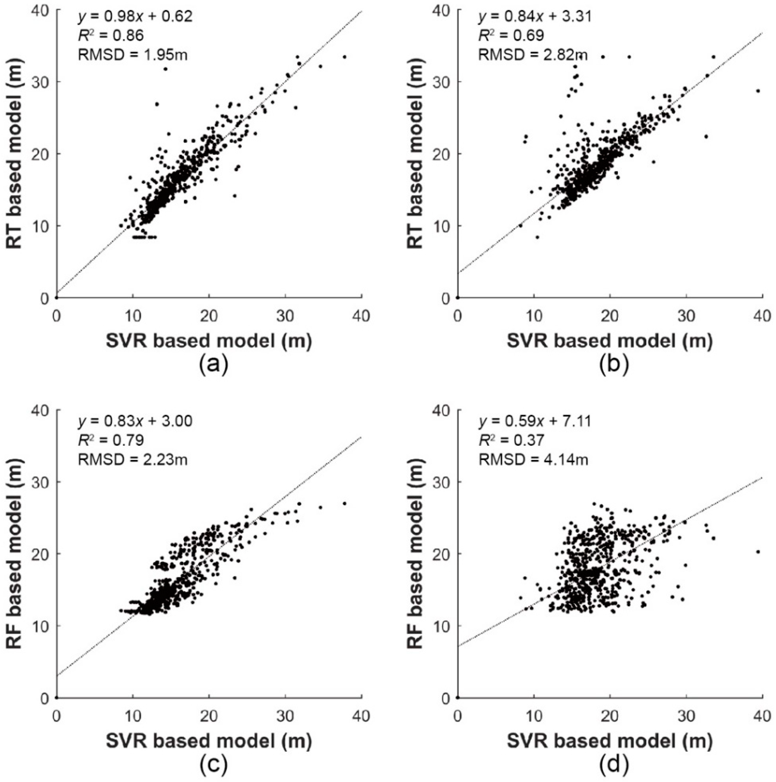
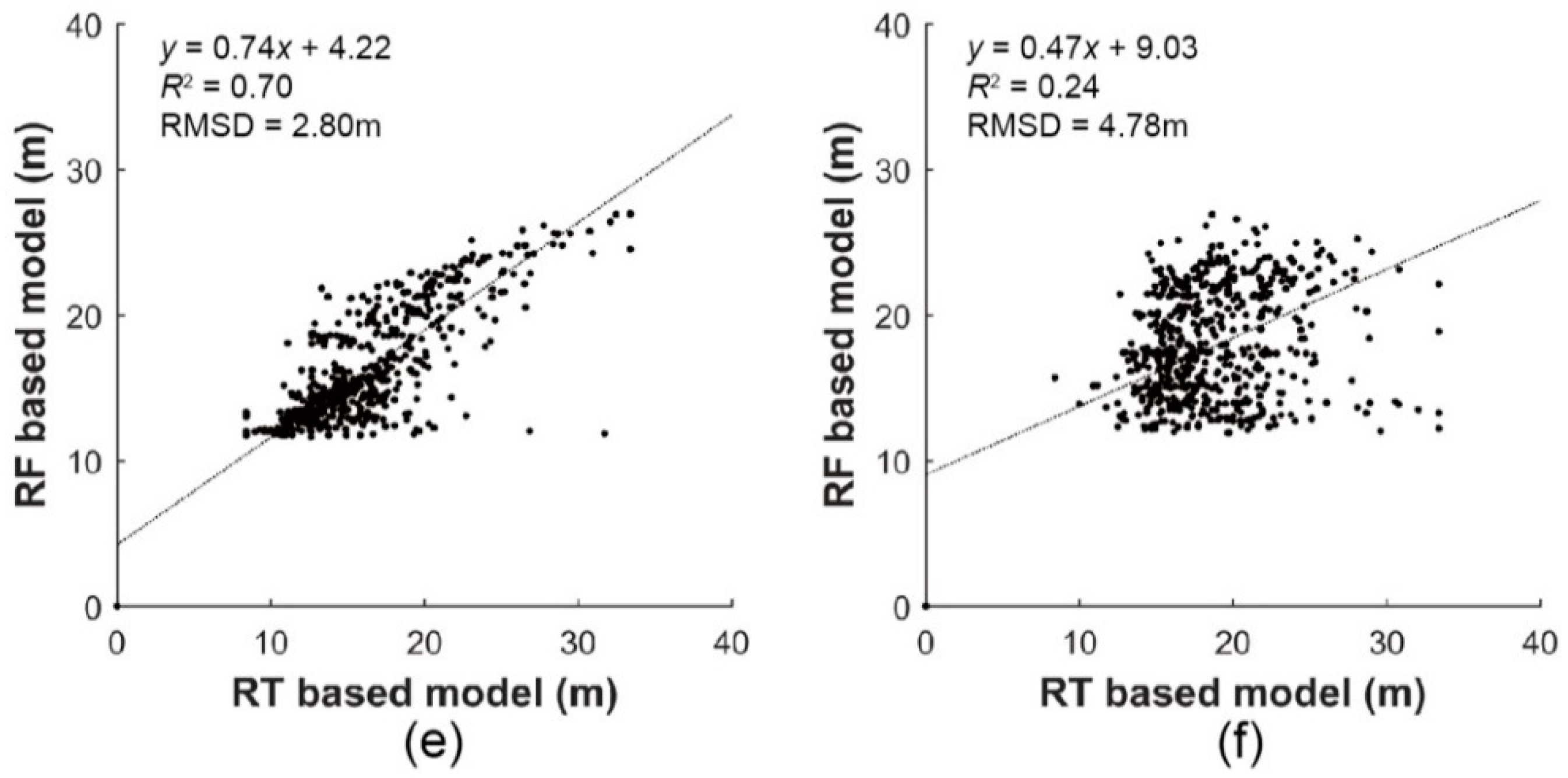
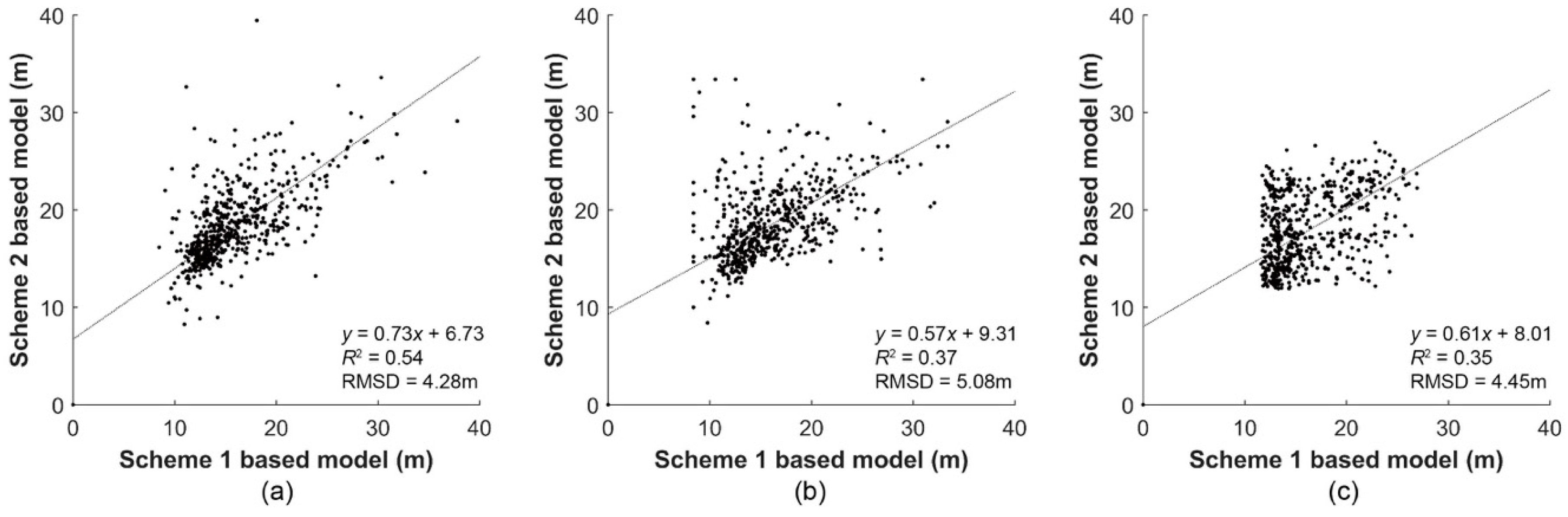
3.2. Inter-Comparison of Stand-Level Height Models
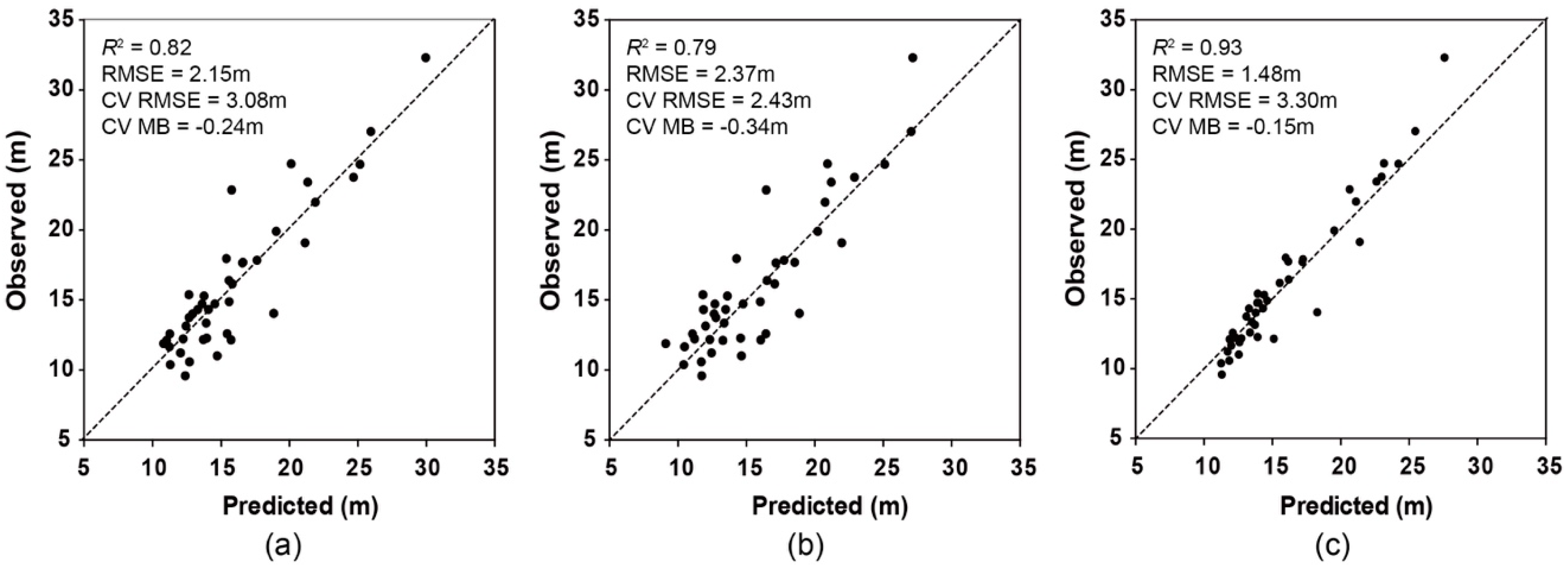
3.3. Validation of Forest Stand Height Models
3.4. Potentials and Limitations
4. Conclusions
Author Contributions
Funding
Conflicts of Interest
References
- Canadell, J.G.; Raupach, M.R. Managing Forests for Climate Change Mitigation. Science 2008, 320, 1456–1457. [Google Scholar] [CrossRef] [PubMed]
- Lindenmayer, D.B.; Margules, C.R.; Botkin, D.B. Indicators of Biodiversity for Ecologically Sustainable Forest Management. Conserv. Biol. 2000, 14, 941–950. [Google Scholar] [CrossRef]
- Gao, T.; Hedblom, M.; Emilsson, T.; Nielsen, A.B. The role of forest stand structure as biodiversity indicator. For. Ecol. Manag. 2014, 330, 82–93. [Google Scholar] [CrossRef]
- Sun, G.; Vose, J.M. Forest management challenges for sustaining water resources in the Anthropocene. Forests 2016, 7, 68. [Google Scholar] [CrossRef]
- Locatelli, B.; Evans, V.; Wardell, A.; Andrade, A.; Vignola, R. Forests and Climate Change in Latin America: Linking Adaptation and Mitigation. Forests 2011, 2, 431–450. [Google Scholar] [CrossRef] [Green Version]
- Shugart, H.H.; Saatchi, S.; Hall, F.G. Importance of structure and its measurement in quantifying function of forest ecosystems. J. Geophys. Res. Biogeosci. 2010, 115. [Google Scholar] [CrossRef]
- Fang, F.; Im, J.; Lee, J.; Kim, K. An improved tree crown delineation method based on live crown ratios from airborne LiDAR data. GISci. Remote Sens. 2016, 53, 402–419. [Google Scholar] [CrossRef]
- Manzanera, J.; Garcia-Abril, A.; Pascual, C.; Tejera, R.; Martin-Fernandez, S.; Tokola, T.; Valbuena, R. Fusion of airborne LiDAR and multispectral sensors reveals synergic capabilities in forest structure characterization. GISci. Remote Sens. 2016, 53, 723–738. [Google Scholar] [CrossRef]
- Chu, H.; Wang, C.; Kong, S.; Chen, K. Integration of full waveform LiDAR and hyperspectral data to enhance tea and areca classification. GISci. Remote Sens. 2016, 53, 542–559. [Google Scholar] [CrossRef]
- Li, M.; Im, J.; Quackenbush, L.J. Forest Biomass and Carbon Stock Quantification Using Airborne LiDAR Data: A Case Study Over Huntington Wildlife Forest in the Adirondack Park. IEEE J. Sel. Top. Appl. Earth Obs. Remote Sens. 2014, 7, 3143–3156. [Google Scholar] [CrossRef]
- Nakai, T.; Sumida, A.; Kodama, Y.; Hara, T.; Ohta, T. A comparison between various definitions of forest stand height and aerodynamic canopy height. Agric. For. Meteorol. 2010, 150, 1225–1233. [Google Scholar] [CrossRef]
- Hyypp, J.; Hyyppä, H.; Leckie, D.; Gougeon, F.; Maltamo, X.Y.M. Review of methods of small-footprint airborne laser scanning for extracting forest inventory data in boreal forests. Int. J. Remote Sens. 2008, 29, 1339–1366. [Google Scholar] [CrossRef]
- Edson, C.; Wing, M.G. Airborne Light Detection and Ranging (LiDAR) for Individual Tree Stem Location, Height, and Biomass Measurements. Remote Sens. 2011, 3, 2494–2528. [Google Scholar] [CrossRef] [Green Version]
- Kaartinen, H.; Hyyppä, J.; Yu, X.; Vastaranta, M.; Hyyppä, H.; Kukko, A.; Holopainen, M.; Heipke, C.; Hirschmugl, M.; Morsdorf, F.; et al. An International Comparison of Individual Tree Detection and Extraction Using Airborne Laser Scanning. Remote Sens. 2012, 4, 950–974. [Google Scholar] [CrossRef] [Green Version]
- Breidenbach, J.; Koch, B.; Kändler, G.; Kleusberg, A. Quantifying the influence of slope, aspect, crown shape and stem density on the estimation of tree height at plot level using lidar and InSAR data. Int. J. Remote Sens. 2008, 29, 1511–1536. [Google Scholar] [CrossRef]
- Yu, X.; Hyyppä, J.; Holopainen, M.; Vastaranta, M. Comparison of Area-Based and Individual Tree-Based Methods for Predicting Plot-Level Forest Attributes. Remote Sens. 2010, 2, 1481–1495. [Google Scholar] [CrossRef]
- Means, J.E.; Acker, S.A.; Fltt, B.J.; Renslow, M.; Emerson, U.; Hendrix, C.J. Predicting Forest Stand Characteristics with Airborne Scanning Lidar. Photogramm. Eng. Remote Sens. 2000, 66, 1367–1371. [Google Scholar]
- Næsset, E.; Bjerknes, K.-O. Estimating tree heights and number of stems in young forest stands using airborne laser scanner data. Remote Sens. Environ. 2001, 78, 328–340. [Google Scholar]
- Næsset, E. Predicting forest stand characteristics with airborne scanning laser using a practical two-stage procedure and field data. Remote Sens. Environ. 2002, 80, 88–99. [Google Scholar] [CrossRef]
- Næsset, E. Practical large-scale forest stand inventory using a small-footprint airborne scanning laser. Scand. J. For. Res. 2004, 19, 164–179. [Google Scholar] [CrossRef]
- Donoghue, D.N.M.; Watt, P.J. Using LiDAR to compare forest height estimates from IKONOS and Landsat ETM+ data in Sitka spruce plantation forests. Int. J. Remote Sens. 2006, 27, 2161–2175. [Google Scholar] [CrossRef]
- Wulder, M.A.; Seemann, D. Forest inventory height update through the integration of lidar data with segmented Landsat imagery. Can. J. Remote Sens. 2003, 29, 536–543. [Google Scholar] [CrossRef]
- Mora, B.; Wulder, M.A.; White, J.C.; Hobart, G. Modeling stand height, volume, and biomass from very high spatial resolution satellite imagery and samples of airborne LiDAR. Remote Sens. 2013, 5, 2308–2326. [Google Scholar] [CrossRef]
- Mora, B.; Wulder, M.A.; Hobart, G.W.; White, J.C.; Bater, C.W.; Gougeon, F.A.; Varhola, A.; Coops, N.C. Forest inventory stand height estimates from very high spatial resolution satellite imagery calibrated with lidar plots. Int. J. Remote Sens. 2013, 34, 4406–4424. [Google Scholar] [CrossRef]
- Vega, C.; Hamrouni, A.; Mokhtari, S.E.; Morel, J.; Bock, J.; Renaud, J.-P.; Bouvier, M.; Durrieu, S. PTrees: A point-based approach to forest tree extraction from lidar data. Int. J. Appl. Earth Obs. Geoinf. 2014, 33, 98–108. [Google Scholar] [CrossRef]
- Khosravipour, A.; Skidmore, A.K.; Wang, T.; Isenburg, M.; Khoshelham, K. Effect of slope on treetop detection using a LiDAR Canopy Height Model. ISPRS J. Photogramm. Remote Sens. 2015, 104, 44–52. [Google Scholar] [CrossRef]
- Laar, A.V.; Akça, A. Forest Mensuration, 2nd ed.; Springer: Dordrecht, The Netherlands, 2007. [Google Scholar]
- Stojanova, D.; Panov, P.; Gjorgjioski, V.; Kobler, A.; Džeroski, S. Estimating vegetation height and canopy cover from remotely sensed data with machine learning. Ecol. Inf. 2010, 5, 256–266. [Google Scholar] [CrossRef]
- Hudak, A.T.; Strand, E.K.; Vierling, L.A.; Byrne, J.C.; Eitel, J.U.H.; Martinuzzi, S.; Falkowski, M.J. Quantifying aboveground forest carbon pools and fluxes from repeat LiDAR surveys. Remote Sens. Environ. 2012, 123, 25–40. [Google Scholar] [CrossRef]
- Shataee, S.; Kalbi, S.; Fallah, A.; Pelz, D. Forest attribute imputation using machine-learning methods and ASTER data: Comparison of k-NN, SVR and random forest regression algorithms. Int. J. Remote Sens. 2012, 33, 6254–6280. [Google Scholar] [CrossRef]
- Richardson, H.; Hill, D.; Denesiuk, D.; Fraser, L. A comparison of geographic datasets and field measurements to model soil carbon using random forests and stepwise regressions (British Columbia, Canada). GISci. Remote Sens. 2017, 54, 573–591. [Google Scholar] [CrossRef]
- Im, J.; Jensen, J.; Coleman, M.; Nelson, E. Hyperspectral remote sensing analysis of short rotation woody crops grown with controlled nutrient and irrigation treatments. Geocarto Int. 2009, 24, 293–312. [Google Scholar] [CrossRef]
- Sonobe, R.; Yamaya, Y.; Tani, H.; Wang, X.; Kobayashi, N.; Mochizuki, K.I. Assessing the suitability of data from Sentinel-1A and 2A for crop classification. GISci. Remote Sens. 2017, 54, 918–938. [Google Scholar] [CrossRef]
- Zhang, C.; Smith, M.; Fang, C. Evaluation of Goddard’s LiDAR, hyperspectral, and thermal data products for mapping urban land-cover types. GISci. Remote Sens. 2017, 55, 1–20. [Google Scholar] [CrossRef]
- Amani, M.; Salehi, B.; Mahdavi, S.; Granger, J.; Brisco, B. Wetland classification in Newfoundland and Labrador using multi-source SAR and optical data integration. GISci. Remote Sens. 2017, 54, 779–796. [Google Scholar] [CrossRef]
- Pham, T.; Yoshino, K.; Bui, D. Biomass estimation of Sonneratia caseolaris (L.) Engler at a coastal area of Hai Phong city (Vietnam) using ALOS-2 PALSAR imagery and GIS-based multi-layer perceptron neural networks. GISci. Remote Sens. 2017, 54, 329–353. [Google Scholar] [CrossRef]
- Omer, G.; Mutanga, O.; Abdel-Rahman, E.M.; Adam, E. Empirical prediction of Leaf Area Index (LAI) of endangered tree species in intact and fragmented indigenous forests ecosystems using WorldView-2 data and two robust machine learning algorithms. Remote Sens. 2016, 8, 324. [Google Scholar] [CrossRef]
- Franklin, S.E.; Ahmed, O.S. Deciduous tree species classification using object-based analysis and machine learning with unmanned aerial vehicle multispectral data. Int. J. Remote Sens. 2017, 38, 1–10. [Google Scholar] [CrossRef]
- Vapnik, V. The Nature of Statistical Learning Theory; Springer Science & Business Media: New York, NY, USA, 2013. [Google Scholar]
- Wang, J.; Neskovic, P.; Cooper, L.N. Training data selection for support vector machines. In International Conference on Natural Computation; Springer: Berlin/Heidelberg, Germany, 2005; pp. 554–564. [Google Scholar]
- Drucker, H.; Burges, C.J.; Kaufman, L.; Smola, A.J.; Vapnik, V. Support vector regression machines. Adv. Neural Inf. Process. Syst. 1997, 9, 155–161. [Google Scholar]
- Mountrakis, G.; Im, J.; Ogole, C. Support vector machines in remote sensing: A review. ISPRS J. Photogramm. Remote Sens. 2011, 66, 247–259. [Google Scholar] [CrossRef]
- Chang, C.C.; Lin, C.J. LIBSVM: A library for support vector machines. ACM Trans. Intell. Syst. Technol. (TIST) 2011, 2, 27. [Google Scholar] [CrossRef]
- RuleQuest. 2012. Available online: http://www.rulequest.com/ (accessed on 10 September 2017).
- Breiman, L. Random forests. Mach. Learn. 2001, 45, 5–32. [Google Scholar] [CrossRef]
- Belgiu, M.; Drăguţ, L. Random forest in remote sensing: A review of applications and future directions. ISPRS J. Photogramm. Remote Sens. 2016, 114, 24–31. [Google Scholar] [CrossRef]
- Chen, Q.; Gong, P.; Baldocchi, D.; Tian, Y.Q. Estimating basal area and stem volume for individual trees from lidar data. Photogramm. Eng. Remote Sens. 2007, 73, 1355–1365. [Google Scholar] [CrossRef]
- Montealegre, A.L.; Lamelas, M.T.; Riva, J.D.L.; García-Martín, A.; Escribano, F. Use of low point density ALS data to estimate stand-level structural variables in Mediterranean Aleppo pine forest. Forestry 2016, 89, 373–382. [Google Scholar] [CrossRef]
- Ahmed, O.S.; Franklin, S.E.; Wulder, M.A.; White, J.C. Characterizing stand-level forest canopy cover and height using Landsat time series, samples of airborne LiDAR, and the Random Forest algorithm. ISPRS J. Photogramm. Remote Sens. 2015, 101, 89–101. [Google Scholar] [CrossRef]


| Sensor Name | Leica ALS60 |
|---|---|
| Laser pulse rate | 85,600 Hz |
| Scan field of view | 25 degree |
| Flying altitude | 1250 m |
| Swath width | 554.24 m |
| Flight line spacing | 217.74 m |
| Footprint diameter | 0.29 m |
| Average point density | 6.25 pts/m2 |
| Number of Trees | Mean Diameter at Breast Height (cm) | Arithmetic Mean Height (m) | Mean Slope (°) | |
|---|---|---|---|---|
| Mean | 27.60 | 24.61 | 16.13 | 24.42 |
| Standard deviation | 15.05 | 8.06 | 5.12 | 8.09 |
| Stand | Number of Trees | Mean Diameter at Breast Height (cm) | Mean Tree Height (m) | Mean Slope (°) | Dominant Tree Species |
|---|---|---|---|---|---|
| A | 88 | 26.57 | 16.32 | 17.11 | Pinus koraiensis Siebold & Zucc., Populus nigra L. |
| B | 47 | 34.31 | 20.34 | 16.82 | Larix kaempferi (Lamb.) Carr. |
| C | 14 | 28.10 | 19.96 | 25.35 | Pinus koraiensis Siebold & Zucc. |
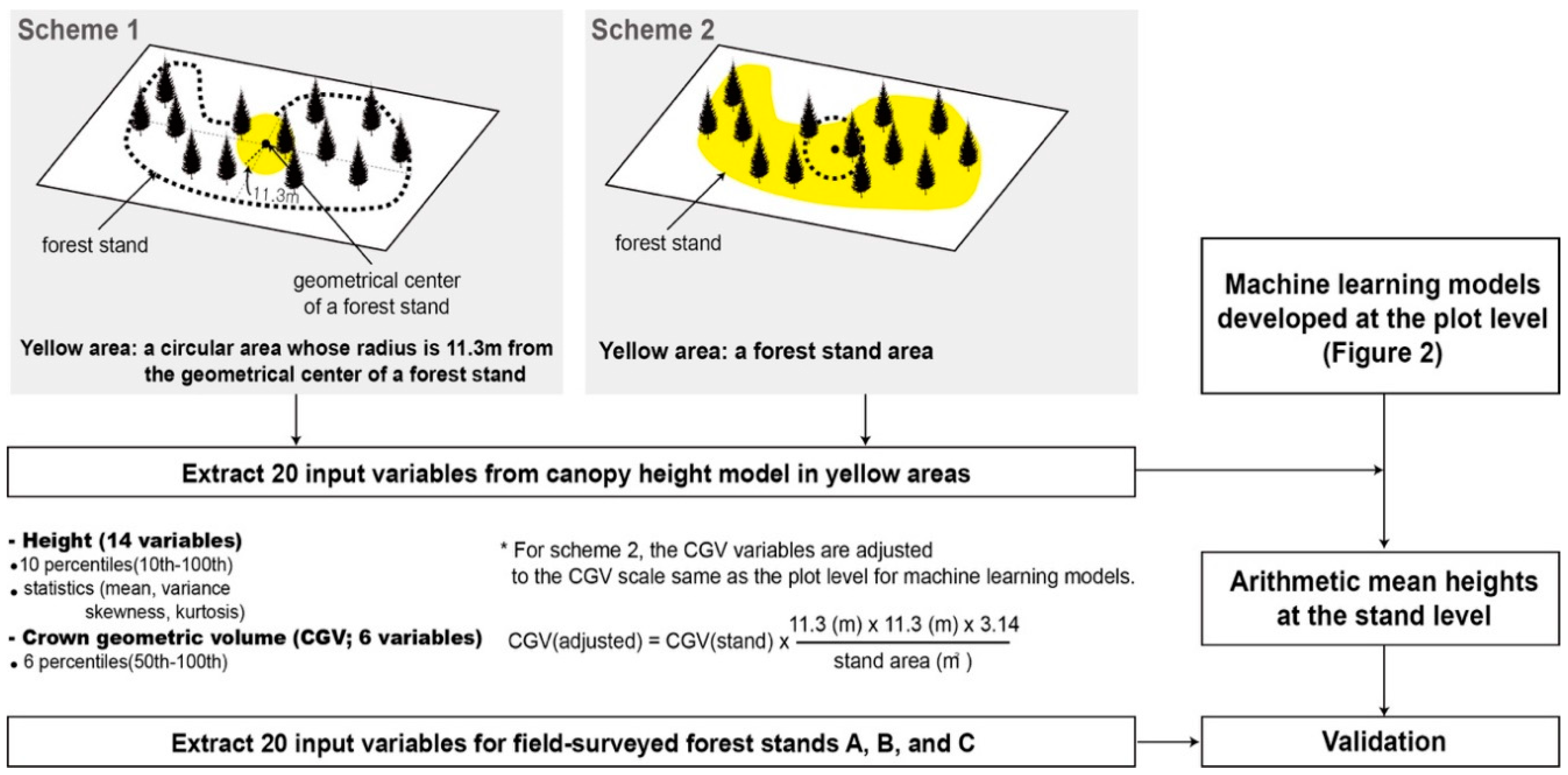
| Variable Type | Variable Explanation | Number of Variables |
|---|---|---|
| Height | 10th to 100th percentiles with interval of 10 | 10 |
| Mean, variance, skewness and kurtosis | 4 | |
| Crown Geometric Volume (CGV) [10,47] | 50th to 100th percentiles with the interval of 10 | 6 |
| Mean Difference (Mean Absolute Difference) | ||||
|---|---|---|---|---|
| Scheme\Model | SVR | RT | RF | Individual Tree-Based |
| Scheme 1 | −0.29 m (3.43 m) | 0.04 m (1.99 m) | −0.94 m (3.22 m) | 0.05 m (1.38 m) |
| Scheme 2 | −0.3 m (0.64 m) | 1.09 m (1.89 m) | 4.69 m (5.04 m) | |
© 2018 by the authors. Licensee MDPI, Basel, Switzerland. This article is an open access article distributed under the terms and conditions of the Creative Commons Attribution (CC BY) license (http://creativecommons.org/licenses/by/4.0/).
Share and Cite
Lee, J.; Im, J.; Kim, K.; Quackenbush, L.J. Machine Learning Approaches for Estimating Forest Stand Height Using Plot-Based Observations and Airborne LiDAR Data. Forests 2018, 9, 268. https://doi.org/10.3390/f9050268
Lee J, Im J, Kim K, Quackenbush LJ. Machine Learning Approaches for Estimating Forest Stand Height Using Plot-Based Observations and Airborne LiDAR Data. Forests. 2018; 9(5):268. https://doi.org/10.3390/f9050268
Chicago/Turabian StyleLee, Junghee, Jungho Im, Kyungmin Kim, and Lindi J. Quackenbush. 2018. "Machine Learning Approaches for Estimating Forest Stand Height Using Plot-Based Observations and Airborne LiDAR Data" Forests 9, no. 5: 268. https://doi.org/10.3390/f9050268