Abstract
Biomass structure is an important feature of terrestrial vegetation. The parameters of forest biomass structure are important for forest monitoring, biomass modelling and the optimal utilization and management of forests. In this paper, we used the most comprehensive database of sample plots available to build a set of multi-dimensional regression models that describe the proportion of different live biomass fractions (i.e., the stem, branches, foliage, roots) of forest stands as a function of average stand age, density (relative stocking) and site quality for forests of the major tree species of northern Eurasia. Bootstrapping was used to determine the accuracy of the estimates and also provides the associated uncertainties in these estimates. The species-specific mean percentage errors were then calculated between the sample plot data and the model estimates, resulting in overall relative errors in the regression model of −0.6%, −1.0% and 11.6% for biomass conversion and expansion factor (BCEF), biomass expansion factor (BEF), and root-to-shoot ratio respectively. The equations were then applied to data obtained from the Russian State Forest Register (SFR) and a map of forest cover to produce spatially distributed estimators of biomass conversion and expansion factors and root-to-shoot ratios for Russian forests. The equations and the resulting maps can be used to convert growing stock volume to the components of both above-ground and below-ground live biomass. The new live biomass conversion factors can be used in different applications, in particular to substitute those that are currently used by Russia in national reporting to the UNFCCC (United Nations Framework Convention on Climate Change) and the FAO FRA (Food and Agriculture Organization’s Forest Resource Assessment), among others.
1. Introduction
Forest biomass is an important input to the monitoring and implementation of the United Nations Sustainable Development Goals [], providing humans with materials and renewable energy, securing carbon stocks, providing links to biodiversity and recreation, and supporting agricultural production. Biomass structure is represented by biomass expansion factors and the root-to-shoot ratio (R:S), which are important characteristics that are used to estimate biomass components based on growing stock volumes (GSV), and to quantify the inter-tree allocation of biomass. The biomass structure of forest ecosystems includes live biomass, which is divided into the live biomass of trees (stands) and the lower layers such as the understory, undergrowth and green forest floor; and dead vegetation matter including standing dry trees (snags), fallen wood (logs), stumps, dead roots and dry branches of live trees. In many cases, the assessment is limited to only the aboveground live biomass of trees, e.g., in applications of remote sensing []. In this paper, we consider live biomass of trees both above- and belowground.
Biomass structure and its indicators are different for different tree species depending on climate and soil conditions, and they vary substantially by forest type, age, levels of productivity, and stand stocking [,,]. Direct measurement of biomass structure is labor intensive and limited to either destructive sampling or the more recently introduced terrestrial LiDAR scanning (with some limitations). However, the limited amount of relevant measurements may lead to substantial biases in the estimates of biomass structure. For example, substantial underestimation of root biomass by Earth system models has been reported previously by Song et al. [].
Above-ground biomass of individual trees or stands is typically assessed by allometric equations [,]. However, existing models do not consider all of the significant factors that control the forest biomass structure. For instance, Forrester et al. [], who provide an overview of existing European biomass models through nearly 1000 models collected in a database, claim that age and stand density are rarely used in the models, yet they are important drivers of biomass structure. The most popular independent variables were tree size, in terms of diameter or height, the number of trees per hectare, the basal area, and climatic parameters (mean annual temperature and mean annual precipitation) []. At the same time, the selection of independent variables in the regression equations depends upon available information. Thus, existing well-elaborated allometric equations [] cannot be used for large scale assessments because they are based on variables (i.e., individual tree diameter and height distribution) that are not available in the aggregated data of forest inventories undertaken at regional and national scales (e.g., the Russian State Forest Register—SFR []).
One of the most important and practical applications of the knowledge of live biomass structure is its assessment for national reporting to the Secretariat of the Intergovernmental Panel on Climate Change (IPCC). The guidance from the IPCC considers the following fractions (Mfr) of forest tree biomass: stem wood over bark (Mst), branches (Mbr), foliage (Mfol) and roots (Mro). “Stem wood over bark” refers to stem wood with bark. Stumps are included in the roots pool, while the tree tops are allocated to the branches. The biomass expansion factor (BEF) is defined as the ratio of aboveground oven-dry biomass (AGB) to either the commercial or stem oven-dry biomass including bark [] (Equation (1)):
The Biomass Conversion and Expansion Factor (BCEF) combine the conversion and expansion processes and help to convert the GSV into AGB [] (Equation (2)) directly:
where D is basic wood density (or specific gravity), in tons of oven-dry matter per m3 stem volume; Mst, Mbr, Mfol are the live biomass of stems, branches, and foliage, respectively, oven-dry t ha−1; and GSV is the growing stock volume in m3. The BCEF has the dimension (t m−3) and can be applied directly to volume-based forest inventory data or remotely sensed estimates without needing information about basic wood densities (and the associated uncertainties). To define belowground live biomass, the IPCC recommends using the root-to-shoot ratio (R:S), i.e., the ratio of the belowground tree live biomass to the aboveground one.
Due to the large extent of Russian forests (more than one-fifth of the global forest area, []), the development of reliable sets of BEFs and BCEFs for Russian forests is interesting from both national and international points of view. There have been noticeable improvements in the models for assessing live biomass and its structure as applied to Russian forests over the last two decades as well as improvements to the amount and distribution of experimental data.
The first set of BEFs for the tree parts of forest ecosystems was published by Alexeyev and Birdsey in 1998 []. The amount and geographical distribution of sample plots were not reported at that time. All BEFs were obtained by graphical fitting of major forest forming species and large geographical regions of Russia. Any numerical conclusions about uncertainties were not reported. Nevertheless, it was the first attempt to present BEFs for assessing the biomass of forest ecosystems over the entire country.
Another team (Zamolodchikov et al.) published a set of BECFs in 2003 [] using a database containing ~2000 sample plots. The sample plots were aggregated (averaged) by 10 dominant species (and two aggregations of softwood and hardwood deciduous tree species) and age groups within three latitudinal belts over the country. The coefficients were applied to data from the SFR and were calculated as mean values by geographic units with corresponding standard errors. In addition to the very large and heterogeneous areas of the latitudinal belts, the study did not consider how much the missing input information (i.e., productivity and stocking) impacted upon the accuracy of the BCEFs.
Usoltsev [,,,] used a constantly growing database of forest biomass measurements to produce a regionalized system of BCEF equations as a function of forest age, average height, average diameter (DBH) and number of trees (N). Equations by Usoltsev can be directly applied to yield tables or individual forest stands where DBH and N are known. However, DBH and N are not contained in the SFR. In order to utilise the SFR data, Usoltsev also provided regional and tree specific regression equations where the BCEF depends on age and GSV []. However, this approach does not consider that the same GSV can have two types of stands: low productive but dense and high productive but sparse, which is critical to the biomass structure. For example, low productive forests invest more in below-ground biomass; sparse forests shift the biomass share from stems to branches (e.g., []).
At the same time, a team at the International Institute for Applied Systems Analysis (IIASA) applied a systems approach to the assessment of BECFs for Russian forests for use of SFR data [] aimed at (1) using all available experimental data collected at that time (about 3500 sample plots), (2) following strict statistical procedures, and (3) decreasing the level of uncertainty by accounting for the specifics of Russian forests and the corresponding forest inventory data. The BECF in this study is based on a non-linear dependence of BCEFfr on indicators available from aggregated data of the SFR: tree species, age, site index and relative stocking. This is the most comprehensive set of parameters that controls forest biomass structure, which are available in the SFR.
More than 10 years have now passed since this publication []. The amount of experimental data available, their spatial distribution and the quality have increased substantially, and new statistical methods have been applied during this period. These advances have therefore driven this research and defined the major objective of this study, i.e., to develop a new, more reliable system for estimating BCEFs and to compare them with those currently used for international reporting by Russia to international bodies such as the IPCC and the Food and Agriculture Organization’s (FAO) Forest Resource Assessment (FRA).
2. Materials and Methods
The methodology consists of two principal steps: (1) estimation of the regression models of forest biomass structure based on field measurements, and (2) development of a map of the spatial distribution of biomass structure indicators using inventory-based biometric characteristics of forest cover.
2.1. Experimental Data
The experimental data used in this assessment consisted of 8007 unique records of sample plots based on destructive biomass sampling. The sample plots were established in the territories of Northern Eurasia and collected in a verified forest biomass database []. The database contained several key indicators of forests (geographical coordinates, dominant tree species, average age, site index, relative stocking, growing stock volume), the mass of live biomass fractions of trees (including stem wood over bark, wood of branches over bark, foliage and roots) and lower forest layers (understory, undergrowth and green forest floor). The data were collected from ca 1200 experiments for the period 1930–2014. Some biomass fractions were sampled more intensively (6315 records for stems, 6441—for branches, 6739—for foliage), while others much less (e.g., 3368—for roots). The accuracy of biomass estimation at the plot level is in the range of 92–94% for stem biomass, 80–90% for the crown and 70–80% for belowground biomass [].
2.2. Forest Biomass Models
The forest biomass measurements from the sample plots [] were used to fit a linear regression model with the logistic transformation of the response to the data of the following form:
where BCEFfr is the biomass conversion and expansion factor for the biomass fraction fr (stems, branches, foliage, roots), which is the ratio of the corresponding biomass fraction to the GSV (t m−3); A is the average stand age in years; RS is the relative stocking (which is the ratio of the basal area of a stand to the basal area of a ‘normal’ stand, i.e., a fully stocked ideal stand based on national standards), typically scaled from 0 to 1 [,]); SI is the site index, which reflects the quality of a site and is expressed by the average height (m) of a mature forest (50 years old for birch and aspen, 160 years old for Siberian pine (Pinus sibirica Du Tour) and 100 years old for other species); and a0–a5 are model parameters. The residual is commonly assumed to have a Gaussian distribution with a zero mean and constant variance.
Equation (3) was selected after examining a number of different analytical expressions that would satisfy a set of general requirements (i.e., statistical significance, analysis of residuals, acceptability of the monotony of dependencies etc.). The logistic transformation of the response allows the BCEF to have values between 0 and 1, which fits the input data (i.e., the database contains values in the range of 0.02–0.95). In principle, Equation (3) can be generalized by replacing 1 with max(BCEF). In this case, the model will allow the response to lie between 0 and the maximum value.
Note that in contrast to classical allometry, Equation (3) allows for the occurrence of extrema by using A and RS twice on the right-hand side of the equation. Extreme BCEFs are not necessarily associated with the maximum (or minimum) values of A and RS. For example, the maximum amount of foliage is not necessarily observed in the densest forests, but rather in medium dense forests. It is known that the maximum mass of leaves on trees is reached at a middle age but not at a mature/overmature age.
A different set of coefficients was fitted for each major forest forming tree species of Northern Eurasia and the above-mentioned biomass fractions were calculated. We obtained a set of BCEF models for stems (BCEFst), branches (BCEFbr), foliage (BCEFfol) and roots (BCEFro) for tree species comprising greater than 98% of the forest cover of Russia. The target variables (BCEF, BEF and R:S) were calculated as following.
where BCEF is the biomass conversion and expansion factor for the entire forest stand (t m−3); BCEFfr is the biomass conversion and expansion factor for the biomass fraction fr (stems, branches, foliage or roots); and R:S is the root-to-shoot ratio.
Due to non-normality and possible heteroscedasticity of the residuals, the model diagnostics and confidence intervals were obtained via non-parametric bootstrapping of 1000 random samples with replacement from the original data, refitting the model for each sample, and evaluating the means and quantiles of the resulting sets of 1000 parameter estimates. The RMSE (root mean squared error) was calculated to assess the accuracy of the model. Also, the species-specific mean percentage errors (MPEs) were evaluated as follows:
where and are observed and estimated values respectively, and is the total number of species-specific observations. The MPEs were thus evaluated for BCEFst, BCEFbr, BCEFfol, BCEFro, BCEF, BEF and R:S. The overall MPEs for each of the above responses were evaluated as weighted averages of species with their respective areal map coverage as weights.
The estimated means and the associated confidence intervals for the maps were obtained by further bootstrapping. All analyses were carried out using R software [], and an example of the code for fitting a model and producing the predictions is provided in the Appendix B.
2.3. Spatial Distribution of the Biomass Structure Parameters
We used the Integrated Land Information System (ILIS) for Russia [], which contains a land cover map [,] and associated forest data that are based on the SFR. The land cover map was developed using a multi-sensor remote sensing approach, geographically weighted regression and reference data obtained using Geo-Wiki []. The ILIS contains the spatial distribution of the forest parameters including the major tree species, the age, the relative stocking and site index, i.e., all the information needed to apply the regression models of forest biomass structure described above. From this, maps of the BCEFs, BEFs and R:S values were produced. The uncertainties associated with the regression equations were also estimated. However, the “overall” uncertainties also depend on the accuracy of the ILIS and SFR, which were not considered here due to lack of information.
3. Results
Using the above-mentioned sample plot database, the parameters of Equation (3) were estimated for the major tree species in Northern Eurasia; these are presented in Table A1. Graphical examples of the equations with the associated 95% confidence envelopes are presented in Figure 1 and Figure 2.
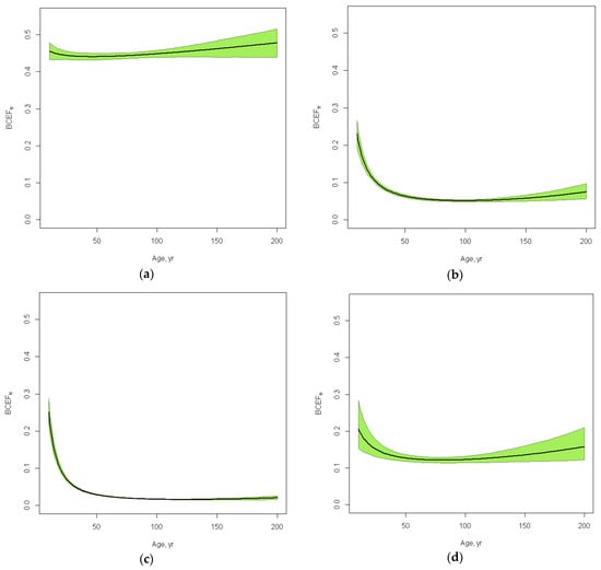
Figure 1.
Estimated biomass conversion and expansion factors (BCEFs) with confidence envelops for (a) stem, (b) branches, (c) foliage and (d) roots in European Russia southern taiga pine forests depending on the stand age with a fixed SI = 21 m and RS = 0.7. In order to build the regression models, we have used 1000 sample plots for stem biomass, 983—for branches, 1038—for foliage and 308—for roots.
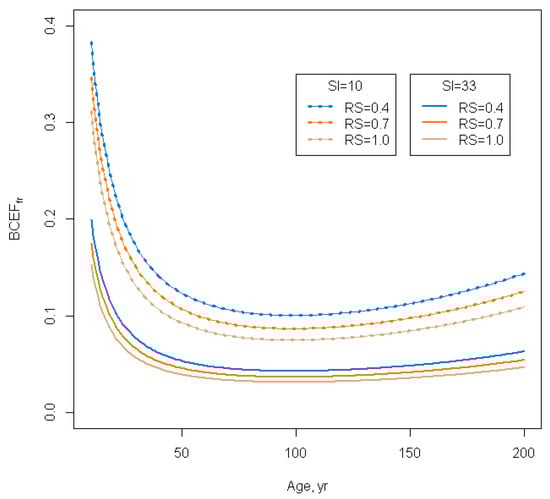
Figure 2.
Biomass conversion and expansion factor for branches in European Russia southern taiga pine forests for different relative stocking values (0.4, 0.7 and 1.0) and site indexes SI (10 m, 33 m). We have used 983 sample plots in order to build the regression model.
Stem BCEFs, which are, in essence, stem wood basic density or specific gravity, do not change much with age in the same site condition; they decrease slightly until the age of 50 and then increase for the remainder of the tree’s life (Figure 1). BCEFs of other fractions (branches, foliage and roots) have a more noticeable drop from young to middle-aged forests because these fractions have a bigger share of young trees. Confidence intervals are wider for very young forests (where there are a variety of reforestation conditions) and for very old forests (where less measurements are available). The share of branches is higher in sparse and low productive forests (Figure 2).
In the next stage, we applied BCEFfr equations to the ILIS land cover map with forest parameters. From this we obtained the spatial distribution of the live biomass structure indicators, including the BCEFs (Figure 3), the BEFs (Figure 4), and the R:S ratios (Figure 5). The maps have resolution of 5 arc second (or 150 m). They can be downloaded in GeoTiff format from Russian Forests and Forestry [] http://webarchive.iiasa.ac.at/Research/FOR/forest_cdrom/english/for_prod_en.html.
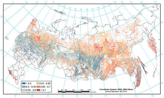
Figure 3.
Geographical distribution of biomass conversion and expansion factors (BCEF, t m−3).
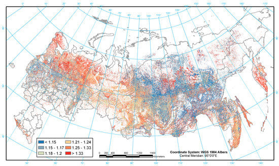
Figure 4.
Geographic distribution of biomass expansion factors (BEF).
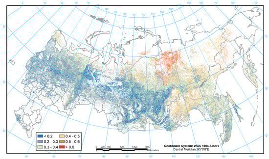
Figure 5.
Geographic distribution of the root-to-shoot ratios.
Relatively high values of the BCEF (Figure 3) for East Siberian forests are mostly related to larch forests with red areas indicating young forests (recently reforested burnt areas) and stone birch (Betula ermanii Cham.) in Kamchatka. The dark blue colors correspond mainly to boreal and temperate pine, spruce and aspen forests. Increased BCEF values in the southern European part of the study region are associated with birch, oak and beech forests. The northern European part of the study region also has relatively high BCEF values because of the dominance of either young or low productive forests.
The BEF is the greater, the large the proportion of branches and foliage in above-ground live biomass, which typical for young or sparse or low productive forests. High BEF values on the map (Figure 4) are also typical for Siberian pine, spruce and fir forests. Low values of BEF are associated with mature forests in general and with alder, pine and larch species in particular.
The R:S ratios are more homogenous across the map (Figure 5) in comparison to the BEFs and BCEFs. Overall the R:S ratios increase with the decreasing productivity of forests, particularly in harsh climates and poorer soil conditions. The highest share of belowground live biomass is observed in larch forests on the continuous permafrost of Central Siberia’s high latitudes where the R:S ratios may reach 0.5–0.6 (including the most northern forests across the globe) while the highly productive forests of the southern taiga and temperate zone have a ratio of around 0.2.
The MPEs used to assess the accuracy of the models are shown in Table 1. The overall relative errors were found to be −0.6%, −1.0% and 11.6% for BCEF, BEF, and R:S ratio respectively.

Table 1.
Relative error of the models (%).
4. Discussion
Accurate estimation of BCEFs with known uncertainties is crucial for GHG inventories and reporting. We applied a two-step approach: (1) build BCEF regression equations depending on the parameters available in both the measurements from sample plots and in the aggregated data from the SFR; (2) apply the regression equations to the SFR data and weight the BCEF by the GSV. The available database of forest biomass measurements is a collection of hundreds of individual studies performed without proper statistical design, which may lead to a bias in the observations. Some tree species were sampled much more intensively then others, and the distribution of forest parameters (e.g., age, tree density, site quality) is different in the available samples compared to the actual forests as reported in the SFR (Figure 6). This is the reason why attempts to use plot averages by tree species and regions by e.g., [], and which is further implemented in the Russian national UNFCCC report 2017 [] and in the guidelines [] approved by the Russian Ministry of Natural Resources and Environment, introduce bias when applied to forest inventory data. Zamolodchikov et al. [] did not consider two important factors of variability in the BCEF: tree density and the level of forest productivity. They assume that sample plots correctly represent the variety of Russian forests, which is not the case (Figure 6c,d). Therefore, the accuracy of the country’s estimates based on the above-mentioned approach cannot be evaluated.
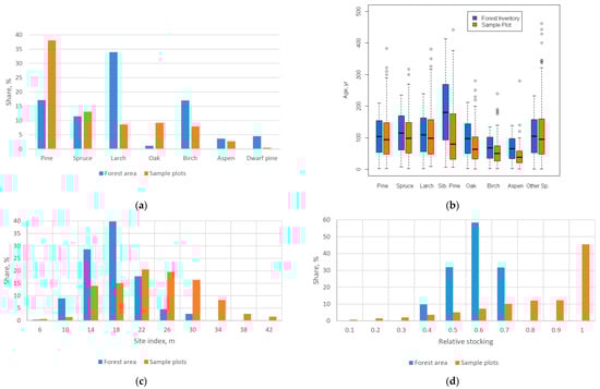
Figure 6.
Discrepancy in sampling: (a) the amount of sample plots by dominant tree species, (b) the age by dominant tree species, (c) the distribution of sample plots by site index and (d) the relative stocking. Total amount of sample plots is 8007, forest area—763 million hectares.
In contrast, this study estimated the BCEFs considering the site index and the tree density distributions of Russian forests. This is why the accuracy of the estimation reported here corresponds to the territorial specifics of the forest cover, which are reflected by the forest inventory data. The total carbon pools and emissions obtained by the BCEFs from this study might (or might not) differ considerably from the current ones [], but our BCEF models are generalizable, because, in additional to species, they take into account SI and RS composition.
A comparison of the BCEFs produced in this study with the ones calculated by Zamolodchikov et al. [] is presented in the appendix (Table A3). Our estimates (Table A3) are higher for some tree species and biomass fractions (e.g., spruce and birch roots, aspen branches), but lower for others (e.g., Siberian pine and fir roots, spruce branches). For example, the difference (between our estimation and []) for the total stand live biomass BCEF of middle taiga middle-aged larch forests is only +9% (Table A3), while stem BCEF is −17%, branches are +69%, foliage is +37% and roots are +138%.
The IPCC 2003 [] report suggests default BEF values (Table 2). Our results (GSV weighted averages) are considerably lower for both boreal and temperate zones. The difference in BEF estimation for boreal coniferous forests (Table 2) might not look substantial (1.35 versus 1.21, i.e., 11.6%); however, this leads to a difference in the live biomass estimation for the entire country of 3.9 million tons.
Table 2.
Comparison of IPCC 2003 [] Tier 1 default BEFs and our (GSV weighted average) estimates for Russia.
The default BCEF values recommended in the IPCC 2006 report are too high for the entire temperate zone due to the variation in Russian tree species and climate conditions across this zone (Table 3). Default BCEF values are also too high for forests with low growing stock (<20 m3 ha−1), e.g., boreal forests at the northern or altitudinal limits, because they can include not only young forests but also sparse and low productive stands.
Table 3.
Comparison of BCEF (t m−3) default values from the IPCC 2006 report with BCEFs calculated using our approach.
The Russian country report for FAO FRA 2015 [] uses a Tier 1 approach to estimate above-ground biomass and Tier 2 for below-ground biomass (Table 4). Our approach satisfies the requirements of Tier 3: “Country-specific national or subnational biomass conversion expansion factors”.
Table 4.
Comparison of BEF, BCEF and R:S calculated using our approach with the FAO FRA country report [].
The R:S ratio suggested by Mokany et al. [] overestimates the data for temperate coniferous forests (Table 5). A major reason for this is because most of the data used for averaging the R:S ratios were collected outside of Russia.
Table 5.
Comparison of the root-to-shoot estimates calculated using our approach with other published values.
All comparisons presented above relate only to trees in stands and they do not consider the lower layers of forest ecosystems (i.e., the understory and green forest floor). Russia has large areas of low productive (mostly northern) forests (around 45% of the area of the country’s major forest forming tree species) where the share of live biomass of the lower layers is substantial (exceeding 10% of the total amount of LB) and should be accounted for within LB inventories. Such models have also been developed, but experimental data are poor and the uncertainties in the corresponding models are high. Even more important is the role of the lower layers of forest ecosystems in the assessments of the Net Primary Production of forests, particularly in methods based on the dynamics of LB components [].
The BCEFs obtained in this study can be used (or tested) in neighboring regions. All available measurements, collected in Ukraine and Belarus, were also used in our regression analysis, so Equation (3) and its parameters (Table A2) are applicable to these two countries. However, regionalized GSV-weighted BCEFs, presented in the Table 1, Table 2, Table 3 and Table 4 and Table A3, need to be calculated based on the forest inventory data of the countries.
5. Conclusions
This study offers a system of equations for estimating forest stand biomass structure and biomass expansion factors for Northern Eurasia, which are more systematic and have lower uncertainties compared to the currently used values for official reporting. The results are presented in the form of spatially distributed multidimensional equations, which use as much relevant information from the forest inventory as possible and are flexible enough that they can be used for different applications. The models are aggregated by species and regions, and satisfy the requirements of both national live biomass inventories and country reporting to international bodies such as the UNFCCC and FAO. The spatial distribution of the BEFs, BCEFs and the R:S ratios were developed based on regression equations and the actual characteristics of the forest cover. The resulting maps can be combined with different remote sensing products (e.g., []) and present spatially distributed information that can be used in further geographical analyses.
Author Contributions
D.S. performed the spatial analysis and wrote the draft of the paper. A.S. designed the study and contributed substantially to the writing of the paper. E.M. designed the statistical analysis and wrote the R-scripts. Y.D., V.B. and O.M. contributed to the statistical analysis. L.S. and F.K. contributed to the writing of the final version of the paper.
Acknowledgments
The study has been partly supported by the DUE GlobBiomass (4000113100/14/I-NB), CCI biomass (4000123662/18/I-NB) and IFBN (4000114425/15/NL/FF/gp) projects funded by ESA; and by the Russian Science Foundation (No. 16-11-00007. We are especially grateful to the inspiring comments received at the International Boreal Forest Research Association (IBFRA—http://ibfra.org) Conference 2015.
Conflicts of Interest
The authors declare no conflict of interest.
Appendix A
Table A1.
Average stand height (m) for different Site Indexes [] Equation (1).
Table A1.
Average stand height (m) for different Site Indexes [] Equation (1).
| Site Index by M.M. Orlov | Birch (50 Years Old Seeding Origin) | Aspen, Poplar, Willow (50 Years, Vegetative Origin) | Siberian Pine (160 Years Old) | Other Species (100 Years Old) |
|---|---|---|---|---|
| If | 34.7–37.5 | 39.5–42.5 | 56.3–60.4 | 49.3–52.9 |
| Ie | 31.8–34.6 | 36.4–39.4 | 52.0–56.2 | 45.6–49.2 |
| Id | 29.0–31.7 | 33.3–36.3 | 47.8–51.9 | 41.9–45.5 |
| Ic | 26.1–28.9 | 30.2–33.2 | 43.6–47.7 | 38.2–41.8 |
| Ib | 23.2–26.0 | 27.1–30.1 | 39.3–43.5 | 34.4–38.1 |
| Ia | 20.3–23.1 | 24.0–27.0 | 35.1–39.2 | 30.7–34.3 |
| I | 17.5–20.2 | 20.9–23.9 | 30.9–35.0 | 27.0–30.6 |
| II | 14.6–17.4 | 17.7–20.8 | 26.6–30.8 | 23.3–26.9 |
| III | 11.7–14.5 | 14.6–17.6 | 22.4–26.5 | 19.6–23.2 |
| IV | 8.9–11.6 | 11.5–14.5 | 18.1–22.3 | 15.9–19.5 |
| V | 6.0–8.8 | 8.4–11.4 | 13.9–18.0 | 12.2–15.8 |
| Va | 3.1–5.9 | 5.3–8.3 | 9.6–13.8 | 8.5–12.1 |
| Vb | 0.2–3.0 | 2.1–5.2 | 5.4–9.5 | 4.0–8.4 |
Table A2.
Parameters of the forest live biomass from Equation (1).
Table A2.
Parameters of the forest live biomass from Equation (1).
| Live Biomass Fraction | Equation (3) Parameter Estimation | r2 | RMSE | N | |||||
|---|---|---|---|---|---|---|---|---|---|
| â0 | â1 | â2 | â3 | â4 | â5 | ||||
| Pine (European middle taiga) | |||||||||
| Stem | 1.3517 | −0.1618 | −0.1443 | 0.1995 | 0.0017 | −0.5163 | 0.14 | 0.072 | 360 |
| Branches | 2.9767 | −1.3238 | −0.349 | −0.4058 | 0.0117 | −0.2093 | 0.58 | 0.039 | 365 |
| Foliage | 5.9603 | −1.4686 | −1.1163 | 0.0122 | 0.006 | −0.5594 | 0.80 | 0.026 | 381 |
| Roots | 2.988 | −0.589 | −0.7742 | −0.0521 | 0.0031 | −0.5536 | 0.50 | 0.071 | 182 |
| Pine (European southern taiga) | |||||||||
| Stem | 0.7717 | −0.0821 | −0.2307 | −0.0568 | 0.0017 | −0.1335 | 0.09 | 0.079 | 1000 |
| Branches | 4.2451 | −1.2431 | −0.7691 | −0.0037 | 0.0127 | −0.5257 | 0.48 | 0.051 | 983 |
| Foliage | 6.6666 | −1.8633 | −1.0966 | 0.0253 | 0.0147 | −0.3913 | 0.77 | 0.045 | 1038 |
| Roots | 1.5704 | −0.5215 | −0.5421 | −0.1002 | 0.0064 | −0.2413 | 0.25 | 0.079 | 308 |
| Pine (European forest steppe) | |||||||||
| Stem | 0.0915 | 0.095 | −0.2237 | −0.0149 | −0.0002 | −0.0021 | 0.07 | 0.069 | 356 |
| Branches | 4.535 | −0.8482 | −1.2881 | 0.074 | 0.0047 | −0.216 | 0.52 | 0.052 | 393 |
| Foliage | 7.0673 | −1.6427 | −1.496 | −0.1959 | 0.0112 | −0.0959 | 0.79 | 0.057 | 423 |
| Roots | −0.2385 | −0.0587 | −0.7152 | −0.6812 | −0.0009 | 0.5308 | 0.21 | 0.032 | 211 |
| Pine (Siberian middle taiga) | |||||||||
| Stem | −0.1346 | 0.1184 | −0.1981 | −0.0839 | −0.0011 | −0.0372 | 0.12 | 0.054 | 158 |
| Branches | 1.0394 | −0.3814 | −0.5978 | 0.2721 | 0.0029 | −1.1483 | 0.31 | 0.025 | 196 |
| Foliage | 7.8944 | −1.4410 | −1.5506 | 0.5492 | 0.0080 | −1.5910 | 0.56 | 0.018 | 196 |
| Roots | −3.2057 | 0.2113 | −0.0074 | −0.2885 | −0.0032 | 0.0286 | 0.04 | 0.031 | 79 |
| Pine (Siberian southern taiga) | |||||||||
| Stem | 0.2432 | 0.1303 | −0.2675 | 0.0493 | −0.0013 | −0.1730 | 0.13 | 0.066 | 586 |
| Branches | 1.1030 | −0.8747 | −0.3201 | −0.6397 | 0.0066 | 0.0227 | 0.50 | 0.036 | 587 |
| Foliage | 5.5623 | −1.7604 | −0.9107 | −0.7045 | 0.0102 | 0.0940 | 0.85 | 0.037 | 582 |
| Roots | 1.7253 | −0.8490 | −0.2326 | 0.2156 | 0.0095 | −0.2221 | 0.19 | 0.092 | 301 |
| Pine (Siberian forest steppe) | |||||||||
| Stem | 1.1294 | −0.0360 | −0.4161 | −0.2785 | 0.0005 | 0.0159 | 0.25 | 0.069 | 163 |
| Branches | 5.1013 | −0.5413 | −1.6572 | −0.8483 | −0.0018 | 0.0194 | 0.64 | 0.065 | 164 |
| Foliage | 8.1398 | −1.5275 | −2.1305 | −1.5911 | 0.0056 | 0.8606 | 0.78 | 0.062 | 164 |
| Roots | 1.7282 | −0.7772 | −0.2703 | 0.2559 | 0.0082 | −0.3057 | 0.19 | 0.091 | 318 |
| Spruce | |||||||||
| Stem | −0.1933 | 0.1173 | −0.1793 | −0.0386 | −0.0012 | 0.0010 | 0.08 | 0.065 | 740 |
| Branches | 3.3337 | −0.7691 | −0.7772 | 0.2153 | 0.0029 | −0.4646 | 0.47 | 0.066 | 767 |
| Foliage | 5.9899 | −1.5668 | −0.8115 | 0.1443 | 0.0084 | −0.6000 | 0.68 | 0.069 | 784 |
| Roots | 1.0646 | −0.4098 | −0.4485 | −0.2869 | 0.0042 | −0.0946 | 0.41 | 0.080 | 401 |
| Fir | |||||||||
| Stem | 0.0959 | −0.0772 | −0.0784 | 0.1718 | 0.0012 | −0.1412 | 0.03 | 0.048 | 262 |
| Branches | 2.3574 | −0.7996 | −0.6041 | 0.0848 | 0.0058 | −0.3075 | 0.35 | 0.031 | 267 |
| Foliage | 4.2704 | −1.3153 | −0.6861 | −0.0233 | 0.0063 | −0.3278 | 0.52 | 0.033 | 279 |
| Roots | 0.6745 | −0.5497 | −0.3379 | 0.3682 | 0.0057 | 0.0503 | 0.38 | 0.032 | 68 |
| Larch (middle taiga) | |||||||||
| Stem | −1.3347 | 0.3120 | 0.0919 | −0.1190 | −0.0023 | 0.0842 | 0.07 | 0.078 | 228 |
| Branches | 0.2162 | −0.7587 | 0.0247 | −0.4946 | 0.0028 | 0.0948 | 0.38 | 0.088 | 227 |
| Foliage | 3.1846 | −1.5464 | −0.4319 | −0.4693 | 0.0062 | 0.1521 | 0.58 | 0.046 | 236 |
| Roots | −2.5068 | 0.1744 | −0.3284 | −1.7051 | −0.0023 | 1.4148 | 0.47 | 0.147 | 60 |
| Larch (southern taiga) | |||||||||
| Stem | 1.1871 | −0.2261 | −0.1119 | 0.0403 | 0.0027 | −0.1945 | 0.08 | 0.079 | 303 |
| Branches | 4.2072 | −1.4826 | −0.6799 | −0.5480 | 0.0118 | 0.2856 | 0.59 | 0.064 | 306 |
| Foliage | 3.6928 | −1.5604 | −0.8472 | −0.5441 | 0.0101 | 0.4642 | 0.61 | 0.033 | 313 |
| Roots | 5.9509 | −0.9601 | −1.2220 | 0.3015 | 0.0098 | −0.7839 | 0.51 | 0.062 | 93 |
| Cedar—Pinus sibirica | |||||||||
| Stem | −0.3297 | −0.0292 | 0.1728 | 0.2949 | 0.0011 | −0.5328 | 0.23 | 0.073 | 161 |
| Branches | 5.3537 | −1.0619 | −0.5370 | 0.7861 | 0.0042 | −2.2664 | 0.61 | 0.040 | 166 |
| Foliage | 8.8813 | −2.1237 | −0.9001 | 0.3048 | 0.0120 | −1.6325 | 0.86 | 0.057 | 166 |
| Roots | 2.2189 | −0.3527 | −0.1341 | 1.1925 | −0.0001 | −2.2136 | 0.28 | 0.031 | 50 |
| Oak | |||||||||
| Stem | 1.3658 | −0.1909 | −0.0649 | 0.0890 | 0.0026 | −0.1504 | 0.02 | 0.096 | 462 |
| Branches | 1.1424 | −0.4008 | −0.7627 | −0.8207 | 0.0031 | 0.6612 | 0.13 | 0.094 | 456 |
| Foliage | 4.1182 | −1.2389 | −1.1572 | −0.4091 | 0.0061 | 0.1719 | 0.67 | 0.030 | 497 |
| Roots | 4.8666 | −0.8227 | −1.2988 | −0.8004 | 0.0056 | 0.6241 | 0.24 | 0.111 | 181 |
| Beech | |||||||||
| Stem | −0.8321 | 0.1425 | 0.2174 | −0.2121 | −0.0018 | 0.1649 | 0.04 | 0.078 | 177 |
| Branches | 0.7318 | 0.0372 | −0.7745 | −0.3449 | −0.0031 | −0.0321 | 0.11 | 0.075 | 146 |
| Foliage | 6.0548 | −1.4001 | −1.3849 | −0.0755 | 0.0063 | −0.6606 | 0.80 | 0.010 | 214 |
| Roots | 1.3070 | −0.3328 | −0.6341 | −0.8082 | −0.0003 | 0.4298 | 0.17 | 0.073 | 112 |
| Hornbeam | |||||||||
| Stem | 2.3347 | 0.3085 | −0.2185 | 2.2934 | −0.0042 | −1.9967 | 0.40 | 0.057 | 38 |
| Branches | 6.3469 | −1.3749 | −1.7074 | 0.1018 | 0.0345 | 0.7156 | 0.27 | 0.086 | 35 |
| Foliage | −1.6432 | −1.0229 | −0.7750 | −3.5763 | 0.0118 | 3.4368 | 0.58 | 0.016 | 38 |
| Roots | 4.6852 | −0.7828 | −1.2655 | −0.7611 | 0.0050 | 0.6045 | 0.24 | 0.110 | 88 |
| Ash | |||||||||
| Stem | −1.4115 | 0.0959 | 0.6140 | 0.5147 | −0.0024 | −0.6225 | 0.20 | 0.058 | 60 |
| Branches | −3.1144 | −0.4433 | 1.0840 | 0.5990 | 0.0033 | −1.2218 | 0.14 | 0.090 | 60 |
| Foliage | 5.7807 | −1.8553 | −0.9758 | −0.1005 | 0.0178 | −0.5541 | 0.63 | 0.100 | 66 |
| Roots | 4.9038 | −0.8047 | −1.3065 | −0.7893 | 0.0052 | 0.5818 | 0.24 | 0.110 | 85 |
| Birch (European Russia) | |||||||||
| Stem | −0.4434 | 0.1641 | 0.0579 | −0.0112 | −0.0037 | −0.0682 | 0.07 | 0.059 | 376 |
| Branches | −0.2754 | −0.4984 | −0.3686 | −0.5492 | 0.0063 | 0.2679 | 0.22 | 0.053 | 407 |
| Foliage | 3.9489 | −1.4559 | −0.9133 | 0.7975 | 0.0174 | −0.6793 | 0.52 | 0.026 | 421 |
| Roots | 1.0270 | −0.3507 | −0.6383 | −0.3961 | −0.0015 | 0.3307 | 0.46 | 0.056 | 169 |
| Birch (Siberia) | |||||||||
| Stem | 0.2318 | 0.0500 | −0.0543 | 0.0179 | −0.0016 | −0.0862 | 0.02 | 0.074 | 215 |
| Branches | −0.7115 | −0.4997 | −0.2326 | −0.6179 | 0.0081 | 0.4321 | 0.21 | 0.041 | 218 |
| Foliage | 0.0304 | −1.0830 | −0.4000 | −0.7894 | 0.0104 | 0.6795 | 0.41 | 0.022 | 225 |
| Roots | 2.2132 | −0.4646 | −0.7980 | −0.0893 | 0.0017 | −0.0285 | 0.41 | 0.070 | 202 |
| Aspen (European Russia) | |||||||||
| Stem | 0.0203 | 0.0012 | −0.0132 | 0.3453 | −0.0006 | −0.2399 | 0.02 | 0.062 | 110 |
| Branches | 0.2000 | −0.2940 | −0.0385 | 1.9673 | 0.0026 | −1.7351 | 0.12 | 0.047 | 123 |
| Foliage | 3.6705 | −1.3091 | −0.9382 | 0.5383 | 0.0137 | −0.7780 | 0.66 | 0.024 | 140 |
| Roots | 2.8964 | −0.3984 | −0.7258 | 0.5918 | −0.0038 | −0.9065 | 0.39 | 0.063 | 43 |
| Aspen (Siberia) | |||||||||
| Stem | −1.2308 | 0.1325 | 0.2480 | 0.3622 | 0.0012 | −0.1355 | 0.14 | 0.075 | 80 |
| Branches | 1.6460 | −0.2113 | −0.6766 | 0.9850 | 0.0021 | −1.4918 | 0.22 | 0.029 | 70 |
| Foliage | 0.3332 | −1.0598 | −0.7049 | −1.5391 | 0.0034 | 1.2358 | 0.80 | 0.010 | 80 |
| Roots | 1.9044 | −0.7256 | −0.7235 | −1.3907 | 0.0036 | 0.8730 | 0.52 | 0.083 | 44 |
| Grey alder | |||||||||
| Stem | −0.0936 | −0.0586 | −0.0101 | −0.0269 | 0.0054 | −0.1466 | 0.18 | 0.057 | 56 |
| Branches | 1.6014 | −0.4444 | −0.9354 | 0.5626 | 0.0070 | −0.5702 | 0.33 | 0.068 | 63 |
| Foliage | −2.0525 | −1.5511 | 0.1970 | −1.7943 | 0.0325 | 1.2196 | 0.72 | 0.016 | 62 |
| Roots | −0.5188 | −0.2344 | −0.3283 | −0.0381 | 0.0084 | −0.3303 | 0.44 | 0.028 | 35 |
| Black alder | |||||||||
| Stem | −0.4665 | 0.2482 | −0.0978 | 0.1064 | −0.0053 | −0.1582 | 0.15 | 0.041 | 87 |
| Branches | −0.7392 | −0.3401 | −0.4609 | −0.1002 | −0.0013 | 0.0418 | 0.14 | 0.018 | 90 |
| Foliage | −0.3775 | −1.1572 | −0.3642 | −1.2107 | 0.0067 | 0.8255 | 0.54 | 0.009 | 90 |
| Roots | −0.5175 | −0.2334 | −0.3350 | −0.0572 | 0.0083 | −0.3157 | 0.44 | 0.028 | 35 |
| Linden | |||||||||
| Stem | −0.5985 | 0.1141 | 0.0629 | 0.1274 | −0.0003 | −0.2424 | 0.29 | 0.038 | 248 |
| Branches | −0.1664 | −0.6651 | −0.1371 | −0.8517 | 0.0035 | 0.0990 | 0.46 | 0.027 | 254 |
| Foliage | 2.7459 | −1.3151 | −1.0017 | −0.8749 | 0.0058 | 0.2103 | 0.77 | 0.011 | 258 |
| Roots | 2.6412 | −0.3251 | −1.0976 | −0.5208 | −0.0018 | 0.2377 | 0.38 | 0.051 | 30 |
| Poplar | |||||||||
| Stem | −1.3420 | 0.3547 | −0.2054 | −0.6031 | −0.0095 | 0.8033 | 0.49 | 0.063 | 89 |
| Branches | −0.3045 | −0.0037 | −0.9988 | −1.5338 | −0.0163 | 1.4965 | 0.43 | 0.114 | 98 |
| Foliage | −0.3746 | −0.8670 | −0.7316 | −1.1603 | −0.0010 | 1.7401 | 0.52 | 0.061 | 86 |
| Roots | −0.6240 | −0.6186 | −0.1614 | −0.8428 | 0.0058 | 1.1717 | 0.87 | 0.013 | 28 |
Table A3.
Comparison of biomass conversion and expansion factors (t m−3) estimated in this study with those of Zamolodchikov et al. (2003).
Table A3.
Comparison of biomass conversion and expansion factors (t m−3) estimated in this study with those of Zamolodchikov et al. (2003).
| Species | Zone | Age Group | BCEF ± SD Our Estimation | BCEF ± SD by Zamolodchikov et al. 2003 | ||||||||
|---|---|---|---|---|---|---|---|---|---|---|---|---|
| Stand | Stem | Branches | Roots | Foliage | Stand | Stem | Branches | Roots | Foliage | |||
| Pine | Northern taiga | Young | 0.919 ± 0.034 | 0.490 ± 0.011 | 0.117 ± 0.008 | 0.178 ± 0.017 | 0.135 ± 0.012 | 0.937 ± 0.118 | 0.469 ± 0.021 | 0.128 ± 0.022 | 0.174 ± 0.031 | 0.167 * ± 0.044 |
| Middle-aged | 0.715 ± 0.012 | 0.474 ± 0.006 | 0.064 ± 0.002 | 0.125 ± 0.006 | 0.051 ± 0.003 | 0.693 ± 0.023 | 0.468 ± 0.010 | 0.052 ** ± 0.002 | 0.143 * ± 0.009 | 0.030 ** ± 0.002 | ||
| Immature | 0.667 ± 0.013 | 0.470 ± 0.006 | 0.058 ± 0.003 | 0.105 ± 0.006 | 0.034 ± 0.002 | 0.737 * ± 0.047 | 0.482 ± 0.016 | 0.067 * ± 0.010 | 0.155 * ± 0.016 | 0.033 ± 0.005 | ||
| Mature | 0.694 ± 0.013 | 0.484 ± 0.006 | 0.065 ± 0.003 | 0.115 ± 0.006 | 0.031 ± 0.002 | 0.661 ± 0.024 | 0.462 ± 0.008 | 0.057 ** ± 0.006 | 0.121 ± 0.008 | 0.021 ** ± 0.002 | ||
| Middle taiga | Young | 0.759 ± 0.030 | 0.452 ± 0.008 | 0.086 ± 0.008 | 0.123 ± 0.013 | 0.098 ± 0.012 | 0.793 ± 0.078 | 0.470 ± 0.027 | 0.131 * ± 0.026 | 0.108 ± 0.013 | 0.084 ± 0.014 | |
| Middle-aged | 0.644 ± 0.010 | 0.454 ± 0.005 | 0.054 ± 0.002 | 0.101 ± 0.005 | 0.035 ± 0.002 | 0.646 ± 0.018 | 0.455 ± 0.006 | 0.062 * ± 0.006 | 0.101 ± 0.004 | 0.028 ** ± 0.002 | ||
| Immature | 0.623 ± 0.011 | 0.454 ± 0.005 | 0.050 ± 0.002 | 0.093 ± 0.005 | 0.026 ± 0.001 | 0.715 * ± 0.052 | 0.475 ± 0.010 | 0.054 ± 0.006 | 0.162 * ± 0.033 | 0.024 ± 0.004 | ||
| Mature | 0.611 ± 0.010 | 0.449 ± 0.005 | 0.052 ± 0.002 | 0.086 ± 0.004 | 0.024 ± 0.001 | 0.646 ± 0.028 | 0.478 * ± 0.014 | 0.054 ± 0.005 | 0.088 ± 0.004 | 0.027 * ± 0.004 | ||
| Southern taiga | Young | 0.725 ± 0.010 | 0.426 ± 0.003 | 0.092 ± 0.002 | 0.134 ± 0.006 | 0.074 ± 0.002 | 0.869 * ± 0.046 | 0.444 ± 0.008 | 0.112 * ± 0.007 | 0.190 * ± 0.019 | 0.123 * ± 0.012 | |
| Middle-aged | 0.627 ± 0.005 | 0.434 ± 0.003 | 0.058 ± 0.001 | 0.109 ± 0.002 | 0.026 ± 0.001 | 0.703 * ± 0.027 | 0.447 ± 0.008 | 0.066 * ± 0.003 | 0.159 * ± 0.014 | 0.032 * ± 0.002 | ||
| Immature | 0.618 ± 0.006 | 0.440 ± 0.003 | 0.051 ± 0.001 | 0.109 ± 0.003 | 0.019 ± 0.0001 | 0.658 * ± 0.021 | 0.453 ± 0.010 | 0.052 ± 0.002 | 0.128 ± 0.007 | 0.026 * ± 0.002 | ||
| Mature | 0.633 ± 0.014 | 0.445 ± 0.006 | 0.053 ± 0.002 | 0.117 ± 0.007 | 0.018 ± 0.001 | 0.712 * ± 0.023 | 0.491 * ± 0.011 | 0.059 ± 0.004 | 0.137 ± 0.007 | 0.025 * ± 0.002 | ||
| Spruce | Northern taiga | Young | 0.971 ± 0.023 | 0.421 ± 0.006 | 0.163 ± 0.008 | 0.211 ± 0.010 | 0.175 ± 0.009 | 0.937 ± 0.068 | 0.413 ± 0.006 | 0.176 ± 0.020 | 0.159 ** ± 0.015 | 0.190 ± 0.027 |
| Middle-aged | 0.815 ± 0.018 | 0.444 ± 0.006 | 0.107 ± 0.004 | 0.193 ± 0.010 | 0.071 ± 0.004 | 0.773 ± 0.039 | 0.457 ± 0.007 | 0.086 ** ± 0.010 | 0.138 ** ± 0.009 | 0.092 * ± 0.013 | ||
| Immature | 0.816 ± 0.019 | 0.450 ± 0.007 | 0.104 ± 0.004 | 0.199 ± 0.011 | 0.063 ± 0.003 | 0.762 ± 0.039 | 0.457 ± 0.010 | 0.086 ** ± 0.009 | 0.150 ** ± 0.012 | 0.069 ± 0.008 | ||
| Mature | 0.779 ± 0.016 | 0.447 ± 0.006 | 0.082 ± 0.003 | 0.205 ± 0.010 | 0.046 ± 0.002 | 0.750 ± 0.039 | 0.457 ± 0.013 | 0.085 * ± 0.008 | 0.163 ** ± 0.015 | 0.045 ± 0.003 | ||
| Middle taiga | Young | 0.930 ± 0.022 | 0.409 ± 0.006 | 0.152 ± 0.007 | 0.198 ± 0.009 | 0.172 ± 0.009 | 0.937 ± 0.068 | 0.413 ± 0.006 | 0.176 * ± 0.020 | 0.159 ** ± 0.015 | 0.190 ± 0.027 | |
| Middle-aged | 0.729 ± 0.011 | 0.426 ± 0.004 | 0.084 ± 0.002 | 0.163 ± 0.006 | 0.055 ± 0.002 | 0.739 ± 0.038 | 0.430 ± 0.009 | 0.099 * ± 0.009 | 0.138 ** ± 0.009 | 0.072 * ± 0.012 | ||
| Immature | 0.718 ± 0.011 | 0.431 ± 0.004 | 0.076 ± 0.002 | 0.166 ± 0.006 | 0.045 ± 0.002 | 0.686 ± 0.026 | 0.465 * ± 0.010 | 0.057 * ± 0.004 | 0.122 ** ± 0.006 | 0.041 ± 0.006 | ||
| Mature | 0.731 ± 0.013 | 0.436 ± 0.005 | 0.070 ± 0.002 | 0.186 ± 0.008 | 0.039 ± 0.001 | 0.681 ** ± 0.030 | 0.444 ± 0.010 | 0.060 * ± 0.003 | 0.139 ** ± 0.013 | 0.038 ± 0.004 | ||
| Southern taiga | Young | 0.837 ± 0.019 | 0.398 ± 0.005 | 0.126 ± 0.006 | 0.174 ± 0.009 | 0.140 ± 0.007 | 1.227 * ± 0.236 | 0.453 * ± 0.032 | 0.182 * ± 0.040 | 0.334 * ± 0.087 | 0.258 * ± 0.077 | |
| Middle-aged | 0.683 ± 0.009 | 0.417 ± 0.004 | 0.072 ± 0.002 | 0.149 ± 0.005 | 0.046 ± 0.001 | 0.737 * ± 0.075 | 0.469 * ± 0.039 | 0.071 ± 0.009 | 0.140 ± 0.019 | 0.056 * ± 0.008 | ||
| Immature | 0.675 ± 0.010 | 0.419 ± 0.004 | 0.067 ± 0.002 | 0.149 ± 0.005 | 0.040 ± 0.001 | 0.702 ± 0.038 | 0.437 ± 0.012 | 0.080 * ± 0.007 | 0.142 ± 0.013 | 0.043 ± 0.006 | ||
| Mature | 0.676 ± 0.010 | 0.424 ± 0.004 | 0.059 ± 0.001 | 0.161 ± 0.006 | 0.032 ± 0.001 | 0.728 * ± 0.027 | 0.452 * ± 0.011 | 0.071 * ± 0.002 | 0.162 ± 0.011 | 0.042 * ± 0.003 | ||
| Fir | all | Young | 0.733 ± 0.046 | 0.371 ± 0.010 | 0.115 ± 0.010 | 0.112 ± 0.021 | 0.132 ± 0.014 | 0.840 ± 0.113 | 0.386 ± 0.033 | 0.123 ± 0.018 | 0.193 * ± 0.033 | 0.138 ± 0.028 |
| Middle-aged | 0.554 ± 0.013 | 0.365 ± 0.005 | 0.067 ± 0.002 | 0.083 ± 0.010 | 0.046 ± 0.002 | 0.615 * ± 0.040 | 0.392 * ± 0.016 | 0.067 ± 0.010 | 0.109 * ± 0.009 | 0.047 ± 0.005 | ||
| Immature | 0.530 ± 0.012 | 0.365 ± 0.004 | 0.061 ± 0.002 | 0.079 ± 0.011 | 0.036 ± 0.001 | 0.565 ± 0.034 | 0.348 ± 0.017 | 0.048 ** ± 0.003 | 0.131 * ± 0.011 | 0.037 ± 0.003 | ||
| Mature | 0.530 ± 0.014 | 0.370 ± 0.005 | 0.060 ± 0.002 | 0.082 ± 0.012 | 0.031 ± 0.001 | 0.539 ± 0.037 | 0.346 ** ± 0.010 | 0.055 ± 0.002 | 0.103 ± 0.024 | 0.035 * ± 0.001 | ||
| Larch | Northern taiga | Young | 1.016 ± 0.088 | 0.492 ± 0.016 | 0.153 ± 0.021 | 0.275 ± 0.057 | 0.096 ± 0.016 | 1.046 ± 0.063 | 0.481 ± 0.016 | 0.068 ** ± 0.013 | 0.456 * ± 0.025 | 0.042 ** ± 0.009 |
| Middle-aged | 0.986 ± 0.054 | 0.547 ± 0.010 | 0.088 ± 0.007 | 0.323 ± 0.041 | 0.028 ± 0.003 | 0.845 ** ± 0.047 | 0.501 ** ± 0.017 | 0.057 ** ± 0.011 | 0.265 ± 0.015 | 0.023 ± 0.005 | ||
| Immature | 0.959 ± 0.047 | 0.559 ± 0.009 | 0.073 ± 0.004 | 0.309 ± 0.037 | 0.018 ± 0.001 | 0.900 ± 0.045 | 0.516 ** ± 0.013 | 0.054 ** ± 0.008 | 0.312 ± 0.021 | 0.019 ± 0.003 | ||
| Mature | 0.926 ± 0.039 | 0.560 ± 0.008 | 0.062 ± 0.003 | 0.291 ± 0.030 | 0.013 ± 0.001 | 0.956 ± 0.044 | 0.531 ± 0.009 | 0.051 ** ± 0.006 | 0.359 ± 0.027 | 0.015 * ± 0.002 | ||
| Middle taiga | Young | 0.983 ± 0.081 | 0.494 ± 0.015 | 0.152 ± 0.020 | 0.247 ± 0.052 | 0.091 ± 0.016 | 0.811 ± 0.166 | 0.621 * ± 0.119 | 0.050 ** ± 0.016 | 0.111 ** ± 0.025 | 0.028 ** ± 0.012 | |
| Middle-aged | 0.914 ± 0.042 | 0.550 ± 0.009 | 0.083 ± 0.005 | 0.259 ± 0.032 | 0.023 ± 0.002 | 0.836 ± 0.125 | 0.661 * ± 0.055 | 0.049 ± 0.007 | 0.109 ** ± 0.061 | 0.017 ± 0.001 | ||
| Immature | 0.909 ± 0.041 | 0.563 ± 0.009 | 0.069 ± 0.003 | 0.262 ± 0.031 | 0.015 ± 0.001 | 0.867 ± 0.162 | 0.648 * ± 0.085 | 0.061 ± 0.007 | 0.131 ** ± 0.061 | 0.027 * ± 0.008 | ||
| Mature | 0.888 ± 0.036 | 0.564 ± 0.008 | 0.060 ± 0.003 | 0.254 ± 0.027 | 0.011 ± 0.001 | 0.807 ± 0.095 | 0.632 * ± 0.029 | 0.055 ± 0.003 | 0.103 ** ± 0.061 | 0.017 * ± 0.002 | ||
| Southern taiga | Young | 0.985 ± 0.063 | 0.516 ± 0.012 | 0.157 ± 0.011 | 0.254 ± 0.046 | 0.057 ± 0.006 | 0.784 ** ± 0.087 | 0.494 ± 0.034 | 0.115 ** ± 0.019 | 0.136 ** ± 0.025 | 0.040 ** ± 0.008 | |
| Middle-aged | 0.735 ± 0.026 | 0.490 ± 0.007 | 0.062 ± 0.003 | 0.166 ± 0.018 | 0.017 ± 0.001 | 0.742 ± 0.112 | 0.524 * ± 0.047 | 0.055 ** ± 0.003 | 0.150 ± 0.061 | 0.013 ** ± 0.001 | ||
| Immature | 0.696 ± 0.025 | 0.486 ± 0.008 | 0.048 ± 0.002 | 0.150 ± 0.016 | 0.012 ± 0.001 | 0.795 * ± 0.112 | 0.575 * ± 0.047 | 0.051 ± 0.003 | 0.156 ± 0.061 | 0.013 ± 0.001 | ||
| Mature | 0.754 ± 0.044 | 0.504 ± 0.012 | 0.053 ± 0.003 | 0.185 ± 0.032 | 0.011 ± 0.001 | 0.795 ± 0.099 | 0.575 * ± 0.030 | 0.051 ± 0.006 | 0.156 ± 0.061 | 0.013 ± 0.003 | ||
| Siberian pine | all | Young | 0.834 ± 0.081 | 0.414 ± 0.011 | 0.136 ± 0.007 | 0.191 ± 0.068 | 0.093 ± 0.005 | 0.783 ± 0.075 | 0.428 ± 0.028 | 0.101 ** ± 0.008 | 0.186 ± 0.028 | 0.068 ** ± 0.011 |
| Middle-aged | 0.663 ± 0.024 | 0.426 ± 0.010 | 0.074 ± 0.005 | 0.135 ± 0.013 | 0.029 ± 0.002 | 0.682 ± 0.057 | 0.413 ± 0.022 | 0.056 ** ± 0.005 | 0.186 * ± 0.028 | 0.027 ± 0.003 | ||
| Immature | 0.653 ± 0.025 | 0.443 ± 0.013 | 0.065 ± 0.006 | 0.117 ± 0.010 | 0.028 ± 0.002 | 0.637 ± 0.054 | 0.393 ** ± 0.027 | 0.061 ± 0.007 | 0.156 * ± 0.016 | 0.027 ± 0.003 | ||
| Mature | 0.663 ± 0.039 | 0.460 ± 0.020 | 0.062 ± 0.010 | 0.108 ± 0.015 | 0.033 ± 0.005 | 0.899 * ± 0.080 | 0.449 ± 0.031 | 0.106 * ± 0.013 | 0.29 * ± 0.031 | 0.045 * ± 0.005 | ||
| Oak seeding | all | Young | 1.165 ± 0.062 | 0.624 ± 0.013 | 0.167 ± 0.018 | 0.311 ± 0.038 | 0.063 ± 0.004 | 1.232 ± 0.137 | 0.569 ** ± 0.016 | 0.116 ** ± 0.009 | 0.485 * ± 0.104 | 0.062 ± 0.008 |
| Middle-aged | 0.966 ± 0.026 | 0.601 ± 0.008 | 0.137 ± 0.007 | 0.206 ± 0.016 | 0.022 ± 0.001 | 0.981 ± 0.060 | 0.594 ± 0.026 | 0.139 ± 0.016 | 0.230 ± 0.017 | 0.018 ** ± 0.002 | ||
| Immature | 0.967 ± 0.030 | 0.603 ± 0.010 | 0.142 ± 0.008 | 0.204 ± 0.018 | 0.018 ± 0.001 | 0.836 ** ± 0.081 | 0.585 ± 0.030 | 0.095 ** ± 0.033 | 0.147 ** ± 0.016 | 0.010 ** ± 0.002 | ||
| Mature | 0.989 ± 0.035 | 0.612 ± 0.011 | 0.150 ± 0.011 | 0.212 ± 0.020 | 0.017 ± 0.001 | 0.956 ± 0.120 | 0.580 ± 0.043 | 0.192 * ± 0.047 | 0.171 ± 0.027 | 0.013 ** ± 0.003 | ||
| Oak coppice | all | Young | 1.453 ± 0.116 | 0.640 ± 0.021 | 0.229 ± 0.038 | 0.466 ± 0.070 | 0.118 ± 0.012 | 1.591 ± 0.104 | 0.671 ± 0.023 | 0.315 * ± 0.024 | 0.403 ± 0.040 | 0.201 * ± 0.017 |
| Middle-aged | 1.075 ± 0.042 | 0.611 ± 0.010 | 0.157 ± 0.011 | 0.269 ± 0.027 | 0.039 ± 0.002 | 1.082 ± 0.133 | 0.604 ± 0.031 | 0.126 ** ± 0.016 | 0.325 ± 0.083 | 0.026 ** ± 0.002 | ||
| Immature | 1.006 ± 0.034 | 0.603 ± 0.010 | 0.148 ± 0.008 | 0.230 ± 0.021 | 0.026 ± 0.001 | 1.125 * ± 0.179 | 0.615 ± 0.032 | 0.176 * ± 0.064 | 0.319 * ± 0.081 | 0.015 ** ± 0.001 | ||
| Mature | 0.979 ± 0.031 | 0.602 ± 0.010 | 0.143 ± 0.008 | 0.212 ± 0.018 | 0.021 ± 0.001 | 1.273 * ± 0.353 | 0.718 * ± 0.155 | 0.225 * ± 0.112 | 0.313 * ± 0.080 | 0.018 ** ± 0.005 | ||
| Other hard deciduous | all | Young | 1.172 ± 0.052 | 0.601 ± 0.011 | 0.176 ± 0.018 | 0.333 ± 0.030 | 0.062 ± 0.005 | 1.248 ± 0.200 | 0.615 ± 0.066 | 0.186 ± 0.038 | 0.392 ± 0.079 | 0.056 ± 0.016 |
| Middle-aged | 1.008 ± 0.033 | 0.597 ± 0.009 | 0.151 ± 0.014 | 0.235 ± 0.015 | 0.025 ± 0.002 | 0.953 ± 0.058 | 0.610 ± 0.026 | 0.143 ± 0.018 | 0.185 ** ± 0.012 | 0.015 ** ± 0.001 | ||
| Immature | 1.021 ± 0.037 | 0.596 ± 0.010 | 0.158 ± 0.014 | 0.245 ± 0.020 | 0.022 ± 0.002 | 0.776 ** ± 0.079 | 0.527 ** ± 0.033 | 0.107 ± 0.018 | 0.129 ** ± 0.026 | 0.013 ** ± 0.003 | ||
| Mature | 1.046 ± 0.045 | 0.608 ± 0.012 | 0.166 ± 0.015 | 0.252 ± 0.026 | 0.020 ± 0.002 | 0.872 ** ± 0.060 | 0.545 ** ± 0.022 | 0.153 ± 0.018 | 0.165 ** ± 0.019 | 0.009 ** ± 0.001 | ||
| Birch | Northern taiga | Young | 1.135 ± 0.066 | 0.534 ± 0.016 | 0.150 ± 0.014 | 0.366 ± 0.042 | 0.085 ± 0.012 | 0.922 ** ± 0.159 | 0.465 ** ± 0.030 | 0.121 ± 0.024 | 0.238 ** ± 0.088 | 0.099 ± 0.017 |
| Middle-aged | 0.976 ± 0.034 | 0.530 ± 0.009 | 0.116 ± 0.008 | 0.284 ± 0.021 | 0.046 ± 0.006 | 0.817 ** ± 0.119 | 0.561 ± 0.069 | 0.053 ** ± 0.021 | 0.180 ** ± 0.019 | 0.024 ** ± 0.011 | ||
| Immature | 0.909 ± 0.029 | 0.537 ± 0.009 | 0.103 ± 0.006 | 0.243 ± 0.019 | 0.026 ± 0.003 | 0.817 ** ± 0.105 | 0.542 ± 0.046 | 0.084 ** ± 0.025 | 0.152 ** ± 0.021 | 0.039 * ± 0.013 | ||
| Mature | 0.889 ± 0.028 | 0.528 ± 0.008 | 0.108 ± 0.006 | 0.227 ± 0.018 | 0.026 ± 0.003 | 0.845 ± 0.089 | 0.523 ± 0.024 | 0.115 ± 0.029 | 0.152 ** ± 0.021 | 0.055 * ± 0.015 | ||
| Middle taiga | Young | 1.012 ± 0.042 | 0.528 ± 0.011 | 0.131 ± 0.009 | 0.287 ± 0.027 | 0.066 ± 0.007 | 0.922 ± 0.159 | 0.465 ** ± 0.030 | 0.121 ± 0.024 | 0.238 ± 0.088 | 0.099 * ± 0.017 | |
| Middle-aged | 0.849 ± 0.017 | 0.534 ± 0.006 | 0.092 ± 0.004 | 0.198 ± 0.010 | 0.026 ± 0.002 | 0.875 ± 0.075 | 0.531 ± 0.013 | 0.103 ± 0.025 | 0.180 ** ± 0.019 | 0.060 * ± 0.018 | ||
| Immature | 0.801 ± 0.013 | 0.533 ± 0.006 | 0.084 ± 0.003 | 0.166 ± 0.007 | 0.018 ± 0.001 | 0.765 ± 0.053 | 0.532 ± 0.026 | 0.057 ** ± 0.003 | 0.152 ± 0.021 | 0.024 * ± 0.003 | ||
| Mature | 0.795 ± 0.018 | 0.528 ± 0.006 | 0.089 ± 0.004 | 0.161 ± 0.011 | 0.017 ± 0.001 | 0.738 ** ± 0.044 | 0.505 ± 0.015 | 0.057 ** ± 0.006 | 0.152 ± 0.021 | 0.024 * ± 0.002 | ||
| Southern taiga | Young | 0.943 ± 0.031 | 0.524 ± 0.008 | 0.118 ± 0.006 | 0.244 ± 0.020 | 0.057 ± 0.004 | 0.873 ** ± 0.047 | 0.496 ± 0.011 | 0.121 ± 0.011 | 0.184 ** ± 0.015 | 0.022 ** ± 0.009 | |
| Middle-aged | 0.806 ± 0.012 | 0.532 ± 0.005 | 0.083 ± 0.003 | 0.169 ± 0.006 | 0.022 ± 0.001 | 0.792 ± 0.024 | 0.539 ± 0.009 | 0.063 ** ± 0.003 | 0.169 ± 0.011 | 0.020 ± 0.001 | ||
| Immature | 0.767 ± 0.010 | 0.532 ± 0.005 | 0.076 ± 0.002 | 0.143 ± 0.005 | 0.016 ± 0.001 | 0.734 ± 0.033 | 0.536 ± 0.014 | 0.061 ** ± 0.004 | 0.123 ** ± 0.015 | 0.014 ± 0.001 | ||
| Mature | 0.761 ± 0.014 | 0.527 ± 0.006 | 0.083 ± 0.003 | 0.137 ± 0.008 | 0.015 ± 0.001 | 0.734 ± 0.045 | 0.531 ± 0.019 | 0.071 ** ± 0.014 | 0.115 ** ± 0.010 | 0.017 * ± 0.002 | ||
| Aspen | all | Young | 0.866 ± 0.073 | 0.403 ± 0.015 | 0.093 ± 0.011 | 0.305 ± 0.054 | 0.065 ± 0.006 | 0.712 ** ± 0.110 | 0.388 ± 0.013 | 0.085 ± 0.016 | 0.179 ** ± 0.062 | 0.059 ± 0.020 |
| Middle-aged | 0.733 ± 0.042 | 0.426 ± 0.012 | 0.080 ± 0.007 | 0.202 ± 0.027 | 0.025 ± 0.002 | 0.726 ± 0.089 | 0.463 * ± 0.019 | 0.063 ** ± 0.005 | 0.179 ± 0.062 | 0.020 ** ± 0.002 | ||
| Immature | 0.686 ± 0.031 | 0.431 ± 0.010 | 0.070 ± 0.006 | 0.167 ± 0.019 | 0.017 ± 0.001 | 0.669 ± 0.114 | 0.432 ± 0.049 | 0.057 ** ± 0.006 | 0.168 ± 0.058 | 0.012 ** ± 0.002 | ||
| Mature | 0.661 ± 0.040 | 0.444 ± 0.017 | 0.069 ± 0.009 | 0.135 ± 0.021 | 0.012 ± 0.001 | 0.730 ± 0.113 | 0.511 * ± 0.052 | 0.052 ** ± 0.005 | 0.157 ± 0.054 | 0.010 ± 0.001 | ||
| Other soft deciduous | all | Young | 0.815 ± 0.044 | 0.415 ± 0.009 | 0.106 ± 0.008 | 0.239 ± 0.032 | 0.055 ± 0.004 | 0.762 ± 0.077 | 0.552 * ± 0.060 | 0.063 ** ± 0.006 | 0.127 ** ± 0.008 | 0.020 ** ± 0.003 |
| Middle-aged | 0.732 ± 0.034 | 0.442 ± 0.005 | 0.077 ± 0.004 | 0.192 ± 0.027 | 0.020 ± 0.001 | 0.672 ± 0.046 | 0.486 * ± 0.030 | 0.047 ** ± 0.006 | 0.129 ** ± 0.008 | 0.011 ** ± 0.002 | ||
| Immature | 0.664 ± 0.022 | 0.450 ± 0.006 | 0.059 ± 0.004 | 0.142 ± 0.015 | 0.013 ± 0.001 | 0.667 ± 0.053 | 0.482 * ± 0.036 | 0.049 ** ± 0.003 | 0.121 ± 0.010 | 0.016 * ± 0.003 | ||
| Mature | 0.682 ± 0.025 | 0.457 ± 0.005 | 0.064 ± 0.004 | 0.150 ± 0.019 | 0.011 ± 0.001 | 0.674 ± 0.032 | 0.482 * ± 0.016 | 0.049 ** ± 0.004 | 0.133 ± 0.009 | 0.010 ± 0.003 | ||
*: the cited value is significantly higher than our estimation, **: it is significantly lower.
Appendix B
R code for regression analysis
- ---
- title: “Fraction Modeling”
- author: “Elena Moltchanova”
- date: “22 September 2017”
- ---
- ```{r echo=F}
- # preliminaries
- rm(list=ls())
- library(MASS)
- setwd(“C:/DM/Article/2018/BEF_RUS/”)
- dat <- read.csv(“DB_plot.csv”,header=T)
- # Example of “DB_plot.csv”, which extracted from Schepaschenko et al., 2017
- # ID,SPEC_MOD,AGE,SI,RS,STEM,BRANCHES,FOLIAGE,ROOTS
- #9436,102,50,32.53,1.47,0.365,0.03093,0.01963,0.02519
- # creating species list
- species.list <- levels(dat[,2])
- vars.list <- names(dat)[6:9]
- Nsim <- 10^3
- Bsim <- 10^3
- # preparing the file for results
- write.table(array(c(‘Species’,’Fraction’,’a0′,’a1′,’a2′,’a3′,’a4′,’a5′,
- ‘a0.sd’,’a1.sd’,’a2.sd’,’a3.sd’,’a4.sd’,’a5.sd’),dim=c(1,14)),file=‘logit_bs_coefs_out.txt’,quote=F,
- row.names=F,col.names=F)
- # preparing array for predicted values
- RS.val <- c(.4,.7,1.0)
- SI.val <- t(array(
- c(37.2, 24.4, 11.7,
- 21.7, 13.1, 4.5,
- 25.5, 16.1, 6.8,
- 32.5, 21.4, 10.2),dim=c(3,4)))
- species.SI.grp <-
- (substr(species.list,1,3)==“105”)*1+(substr(species.list,1,3)%in%c(“124”,”126”,”127”))*2+
- (substr(species.list,1,3)%in%c(“125”,”131”))*3
- species.SI.grp[species.SI.grp==0] <- 4
- #table(species.SI.grp,species.list)
- # FITTING LOGISTIC MODEL WITH BOOTSTRAP
- Nsp <- length(species.list)
- for(j in 1:Nsp){
- dat.curr <- dat[dat[,2]==species.list[j],]
- for(k in 1:4){
- dat.curr$Y <- dat.curr[,5+k]
- is.in.Y <- (!is.na(dat.curr$Y))&(!is.na(dat.curr$AGE))&(!is.na(dat.curr$SI))&(!is.na(dat.curr$RS))
- if(sum(is.in.Y)!=0){
- boot.dat.curr <- dat.curr[is.in.Y,]
- plot(boot.dat.curr$AGE,boot.dat.curr$Y,pch=1,lwd=2,ylim=c(0,1),
- xlim=c(0,210),xlab=‘Age’,ylab=‘Fraction’,
- main=paste(‘Species = ‘,species.list[j],’, Variable = ‘, vars.list[k],sep=‘‘))
- co1b <- array(dim=c(Bsim,6))
- for(biter in 1:Bsim){
- bootdat <- boot.dat.curr[sample(1:dim(boot.dat.curr)[1],replace=T),]
- m1b <- lm(log(Y/(1-Y)) ~ log(AGE)+log(SI)+log(RS)+AGE+RS, data=bootdat)
- co1b[biter,] <- m1b$coef
- }
- # estimating the mean from the coefs.
- mn1b <- apply(co1b,2,mean,na.rm=T)
- sd1b <- apply(co1b,2,sd,na.rm=T)
- AGE.val <- seq(10,210,10); n.age <- length(AGE.val)
- Y.mn1b <- Y.lo1b <- Y.hi1b <- array(dim=c(3,3,n.age))
- for(rs.i in 1:3){
- for(si.i in 1:3){
- for(m in 1:n.age){
- Y.sim <- 1/(1+exp(-(co1b[,1]+co1b[,2]*log(AGE.val[m])+
- co1b[,3]*log(SI.val[species.SI.grp[j],si.i])+co1b[,4]*log(RS.val[rs.i])+
- co1b[,5]*AGE.val[m]+co1b[,6]*RS.val[rs.i])))
- Y.mn1b[rs.i,si.i,m] <- mean(Y.sim,na.rm=T)
- Y.lo1b[rs.i,si.i,m] <- quantile(Y.sim,.025,na.rm=T)
- Y.hi1b[rs.i,si.i,m] <- quantile(Y.sim,.975,na.rm=T)
- }}}
- ### adding non-parametric estimates for CI
- # comparing CIs
- par(mfrow=c(1,1))
- plot(AGE.val,Y.mn1b[1,1,],pch=16,ty=‘o’,xlab=‘age’,ylab=expression(F[st]),ylim=c(0,1),
- main=paste(“SI=“,SI.val[species.SI.grp[j],1]))
- polygon(c(AGE.val,AGE.val[n.age:1]),c(Y.lo1b[1,1,],Y.hi1b[1,1,n.age:1]),density=7,
- angle=25,col=‘magenta’,border=‘magenta’)
- lines(AGE.val,Y.mn1b[1,1,],pch=1,ty=‘o’,col=‘magenta’)
- write.table(array(c(species.list[j],vars.list[k],round(mn1b,4),round(sd1b,4)),dim=c(1,14)),
- file=‘logit_bs_coefs_out.txt’,quote=F,
- row.names=F,col.names=F,append=T)
- }}}
- ```
- \newpage
- ## Estimated Coefficients for the Logit-linear model (Bootstrap)
- ```{r echo=F}
- t3 <- read.table(‘logit_bs_coefs_out.txt’,header=T)
- print(t3[,1:7])
- print(t3[,c(1:2,9:14)])
- ```
Acronyms
| A | average stand age, years |
| AGB | aboveground oven-dry live biomass, t ha−1 |
| BCEF | Biomass Conversion and Expansion Factor, t m−3 |
| BEF | biomass expansion factor, dimensionless |
| DBH | average diameter at breast height, cm |
| GSV | growing stock volume, m3 ha−1 |
| ILIS | Integrated Land Information System |
| IPCC | Intergovernmental Panel on Climate Change |
| FAO FRA | Food and Agriculture Organization’s Forest Resource Assessment |
| Mfr | live biomass of fraction fr, t ha−1 |
| Mst | live biomass of stem wood and bark, t ha−1 |
| Mbr | live biomass of tree branches, t ha−1 |
| Mfol | live biomass of tree foliage, t ha−1 |
| Mro | live biomass of stamp and roots, t ha−1 |
| RMSE | root mean squared error |
| R:S | root-to-shoot ratio |
| RS | relative stocking, typically scaled from 0 to 1—ratio of the basal area of a stand to the basal area of a ‘normal’ stand, i.e., a fully stocked ideal stand based on national standards [,] |
| SI | site index, which reflects the quality of a site and is expressed by the average height (m) of a mature forest (50 years old for birch and aspen, 160 years old for Siberian pine (Pinus sibirica) and 100 years old for other species); and a0–a5 are model parameters. |
| SFR | Russian State Forest Register |
| UNFCCC | United Nations Framework Convention on Climate Change |
References
- Müller, A.; Weigelt, J.; Götz, A.; Schmidt, O.; Alva, I.L.; Matuschke, I.; Ehling, U.; Beringer, T. The Role of Biomass in the Sustainable Development Goals: A Reality Check and Governance Implications; IAS Working Paper; IASS: Potsdam, Germany, 2015; p. 36. [Google Scholar]
- Santoro, M.; Beaudoin, A.; Beer, C.; Cartus, O.; Fransson, J.E.S.; Hall, R.J.; Pathe, C.; Schmullius, C.; Schepaschenko, D.; Shvidenko, A.; et al. Forest growing stock volume of the northern hemisphere: Spatially explicit estimates for 2010 derived from Envisat ASAR. Remote Sens. Environ. 2015, 168, 316–334. [Google Scholar] [CrossRef]
- Shvidenko, A.Z.; Nilsson, S.; Stolbovoi, V.S.; Gluck, M.; Shchepashchenko, D.G.; Rozhkov, V.A. Aggregated estimation of the basic parameters of biological production and the carbon budget of Russian terrestrial ecosystems: 1. Stocks of plant organic mass. Russ. J. Ecol. 2000, 31, 371–378. [Google Scholar] [CrossRef]
- Shepashenko, D.; Shvidenko, A.; Nilsson, S. Phytomass (live biomass) and carbon of Siberian forests. Biomass Bioenergy 1998, 14, 21–31. [Google Scholar] [CrossRef]
- Shvidenko, A.; Schepaschenko, D.; Nilsson, S.; Bouloui, Y. Semi-empirical models for assessing biological productivity of Northern Eurasian forests. Ecol. Model. 2007, 204, 163–179. [Google Scholar] [CrossRef]
- Song, X.; Hoffman, F.M.; Iversen, C.M.; Yin, Y.; Kumar, J.; Ma, C.; Xu, X. Significant inconsistency of vegetation carbon density in CMIP5 Earth system models against observational data. J. Geophys. Res. Biogeosciences 2017, 122, 2282–2297. [Google Scholar] [CrossRef]
- Chave, J.; Réjou-Méchain, M.; Búrquez, A.; Chidumayo, E.; Colgan, M.S.; Delitti, W.B.C.; Duque, A.; Eid, T.; Fearnside, P.M.; Goodman, R.C.; et al. Improved allometric models to estimate the aboveground biomass of tropical trees. Glob. Chang. Biol. 2014, 20, 3177–3190. [Google Scholar] [CrossRef] [PubMed]
- Usoltsev, V. Single-Tree Biomass Data for Remote Sensing and Ground Measuring of Eurasian Forests. CD-Version in English and Russian; Ural State Forest Engineering University: Yekaterinburg, Russia, 2016; ISBN 978-5-94984-600-1. [Google Scholar]
- Forrester, D.I.; Tachauer, I.H.H.; Annighoefer, P.; Barbeito, I.; Pretzsch, H.; Ruiz-Peinado, R.; Stark, H.; Vacchiano, G.; Zlatanov, T.; Chakraborty, T.; et al. Generalized biomass and leaf area allometric equations for European tree species incorporating stand structure, tree age and climate—ScienceDirect. For. Ecol. Manag. 2017, 396, 160–175. [Google Scholar] [CrossRef]
- Usoltsev, V.A.; Chasovskikh, V.P.; Noritsina, Y.V.; Noritsin, D.V. Allometric Models of Tree Biomass for Airborne Laser Scanning and Ground Inventory of Carbon Pool in the Forests of Eurasia: Comparative Analysis. Sib. J. For. Sci. 2016, 3, 68–76. [Google Scholar] [CrossRef]
- Gordov, E.P.; Bryant, K.; Bulygina, O.N.; Csiszar, I.; Eberle, J.; Fritz, S.; Gerasimov, I.; Gerlach, R.; Hese, S.; Kraxner, F.; et al. Development of Information-Computational Infrastructure for Environmental Research in Siberia as a Baseline Component of the Northern Eurasia Earth Science Partnership Initiative (NEESPI) Studies. In Regional Environmental Changes in Siberia and Their Global Consequences; Springer Environmental Science and Engineering; Springer: New York, NY, USA, 2013; pp. 19–56. ISBN 978-94-007-4569-8. [Google Scholar]
- Intergovernmental Panel on Climate Change (IPCC). Good Practice Guidance for Land Use, Land-Use Change and Forestry; Institute for Global Environmental Strategies: Kanagawa Prefecture, Japan, 2003. [Google Scholar]
- Intergovernmental Panel on Climate Change (IPCC). 2006 IPCC Guidelines for National Greenhouse Gas Inventories; IGES: Hayama, Japan, 2006; ISBN 4-88788-032-4. [Google Scholar]
- Food and Agriculture Organization (FAO). Russian Federation—Global Forest Resources Assessment 2015—Country Report; Global Forest Resources Assessment Country Reports; FAO: Rome, Italy, 2014. [Google Scholar]
- Alexeyev, V.A.; Birdsey, R.A. Carbon Storage in Forests and Peatlands of Russia; General Technical Report NE-244; USDA, Forest Service, Northeast Research Station: Radnor, PA, USA, 1998. [Google Scholar]
- Zamolodchikov, D.G.; Utkin, A.I.; Chestnych, O.V. Biomass conversion and expansion factors for major forest forming species in Russia. For. Mensurat. For. Invent. 2003, 1, 119–127. Available online: http://old.cepl.rssi.ru/publications/pub_lab1/zamolodchikov%2003%20koefficienty%20konversii%20zapasov%20v%20fitomassu.pdf (accessed on 25 May 2018).
- Usoltsev, V.A. Growth and Structure of Forest Live Biomass; Nauka: Novosibirsk, Russia, 1988; ISBN 5-02-028865-9. [Google Scholar]
- Usoltsev, V.A. Forming Databanks about Live Biomass of Forests; Russian Academy of Sciences: Ekaterinburg, Russia, 1998; ISBN 5-7691-0832-0. [Google Scholar]
- Usoltsev, V.A. Forest Biomass of Northern Eurasia: Mensuration Standards and Geography; Ural Branch of RAS: Yekaterinburg, Russia, 2002; ISBN 5-7691-1278-6. [Google Scholar]
- Usoltsev, V.A. Biological Productivity of North Eurasian Forests: Methods, Database and Its Applications; Ural Branch of Russian Academy of Science: Ekaterinburg, Russia, 2007; ISBN 5-7691-1757-5. [Google Scholar]
- Schepaschenko, D.; Shvidenko, A.; Usoltsev, V.; Lakyda, P.; Luo, Y.; Vasylyshyn, R.; Lakyda, I.; Myklush, Y.; See, L.; McCallum, I.; et al. A dataset of forest biomass structure for Eurasia. Sci. Data 2017, 4, 170070. [Google Scholar] [CrossRef] [PubMed]
- Shvidenko, A.Z.; Schepaschenko, D.G.; Nilsson, S.; Buluy, Y.I. Tables and Models of Growth and Productivity of Forests of Major Forest Forming Species of Northern Eurasia. Standard and Reference Materials, 2nd ed.; Federal Agency of Forest Management: Moscow, Russia, 2008.
- R Core Team. R: A Language and Environment for Statistical Computing; R Foundation for Statistical Computing: Vienna, Austria, 2013. [Google Scholar]
- Schepaschenko, D.; McCallum, I.; Shvidenko, A.; Fritz, S.; Kraxner, F.; Obersteiner, M. A new hybrid land cover dataset for Russia: A methodology for integrating statistics, remote sensing and in situ information. J. Land Use Sci. 2011, 6, 245–259. [Google Scholar] [CrossRef]
- Schepaschenko, D.; Shvidenko, A.Z.; Lesiv, M.Y.; Ontikov, P.V.; Shchepashchenko, M.V.; Kraxner, F. Estimation of forest area and its dynamics in Russia based on synthesis of remote sensing products. Contemp. Probl. Ecol. 2015, 8, 811–817. [Google Scholar] [CrossRef]
- See, L.; Fritz, S.; Perger, C.; Schill, C.; McCallum, I.; Schepaschenko, D.; Duerauer, M.; Sturn, T.; Karner, M.; Kraxner, F.; et al. Harnessing the power of volunteers, the internet and Google Earth to collect and validate global spatial information using Geo-Wiki. Technol. Forecast. Soc. Chang. 2015, 98, 324–335. [Google Scholar] [CrossRef]
- Shvidenko, A.; Schepaschenko, D.; McCallum, I.; Nilsson, S. Russian Forests and Forestry. Available online: http://www.iiasa.ac.at/Research/FOR/forest_cdrom (accessed on 25 May 2018).
- Nakhutin, A.I.; Gitarskii, M.L.; Romanovskaya, A.A.; Ginzburg, V.A.; Govor, I.L.; Grabar, V.A.; Imshennik, E.V.; Karaban’, R.T.; Korotkov, V.N.; Uvarova, N.E.; et al. National Report on the Cadastre of Anthropogenic Emissions from Sources and Absorptions by Sinks of Greenhouse Gases of Russian Federation Not Regulated by Montreal Protocol for 1990–2015; Institute of Global Climate and Ecology of the Federal Service for Hydrometeorology and Environmental Monitoring and the Russian Academy of Sciences: Moscow, Russia, 2017; p. 471.
- Guideline for Quantification of Greenhouse Gas Absorption; Ministry of Natural Resources and Environment of the Russian Federation: Moscow, Russia, 2017.
- Mokany, K.; Raison, R.J.; Prokushkin, A.S. Critical analysis of root: Shoot ratios in terrestrial biomes. Glob. Chang. Biol. 2006, 12, 84–96. [Google Scholar] [CrossRef]
- Santoro, M.; Beer, C.; Cartus, O.; Schmullius, C.; Shvidenko, A.; McCallum, I.; Wegmüller, U.; Wiesmann, A. Retrieval of growing stock volume in boreal forest using hyper-temporal series of Envisat ASAR ScanSAR backscatter measurements. Remote Sens. Environ. 2011, 115, 490–507. [Google Scholar] [CrossRef]
© 2018 by the authors. Licensee MDPI, Basel, Switzerland. This article is an open access article distributed under the terms and conditions of the Creative Commons Attribution (CC BY) license (http://creativecommons.org/licenses/by/4.0/).