Leaf Temperature Fluctuations of Typical Psammophytic Plants and Their Application to Stomatal Conductance Estimation


1
Yanchi Ecology Research, School of Soil and Water Conservation, Beijing Forestry University, Beijing 100083, China
2
Key Laboratory of State Forestry Administration on Soil and Water Conservation, Beijing Forestry University, Beijing 100083, China
*
Author to whom correspondence should be addressed.
Forests 2018, 9(6), 313; https://doi.org/10.3390/f9060313
Submission received: 26 March 2018
/
Revised: 23 May 2018
/
Accepted: 26 May 2018
/
Published: 1 June 2018
(This article belongs to the Section Forest Ecophysiology and Biology)
Abstract
:Monitoring of stomatal conductance to water vapor in psammophytes is important in studies of vegetation transpiration in sandy areas. Leaf temperature monitoring has the advantages of convenience, reduced damage to the plant without contact, and a larger measurement area. Stomatal conductance to water vapor estimation models, based on leaf temperature, have been proposed in agricultural studies in recent years. However, observations for verification of these models are still lacking, which has limited the application of these models. We performed a drought stress experiment on three typical psammophytes: Artemisia ordosica, Salix psammophila, and Caragana korshinskii. We monitored their leaf temperature and built two leaf temperature-based models to test whether the models could accurately estimate stomatal conductance. Results verified that neither of the two models accurately quantified psammophytes’ stomatal conductance in field operations. We further tested the differences among plants and identified that the differences in stomatal mechanism and physical morphology of the leaves drives leaf temperature differences, which affects the accuracy of stomatal conductance estimation using the models. We concluded that more precise measurements of leaf temperature-related parameters, such as wind speed and leaf physical morphology, are needed to improve the models’ estimation accuracy. Our study offers references for developing a practical application of stomatal conductance estimation models in field operations.
1. Introduction
The plant stomata functions in regulating both gas exchange and water balance [1]. Stomatal conductance to water vapor is an important indicator of the water exchange rate between the plant and the outside environment [2]. For plants that grow in sand, water is the most important growth-limiting factor; therefore, understanding the water vapor exchange rate of sand-grown plants is essential. Monitoring plant stomatal conductance to water vapor, and exploring its patterns in sandy environments, is essential for understanding transpirational water consumption in sandy vegetation, as well as for understanding water circulation in sand.
Leaf temperature is an important physiological index used in plant studies [3,4]. Leaf temperature monitoring methods are simple and convenient, and damage to the plant is negligible because leaf contact is not necessary. The leaf temperature monitoring methods can measure a group of leaves, thus, reducing the overall sampling error [5,6]. The question of whether it is possible to make stomatal conductance simulation easier by taking advantage of this leaf temperature monitoring method for estimating stomatal conductance has been posed in plant physiological ecology studies in recent years [7].
Research has shown that leaf temperature changes occur, in part, in response to stomatal opening and closing. Under conditions of sufficient water, opening of the stomata raises stomatal conductance to water vapor, while evaporative cooling simultaneously lowers leaf temperature, and water vapor is lost through the stomata [8]. In contrast, under water-stressed conditions, closing of the stomata reduces evaporative cooling and leaf temperature increases [9]. Based on this basic law, a series of stomatal conductance estimation methods have been proposed in agricultural research based on leaf temperatures [10]. Two models, the crop water stress index (CWSI) and stomatal conductance index (IG) models, have been shown to be useful through theoretical and experimental studies.
Idso et al. proposed the CWSI model in 1981 [11]. The CWSI model has been applied in agricultural production. Maes and Steppe conducted CWSI research using infrared remote sensing data to reflect the degree of water deficit [12]. Furthermore, Blum et al. built a regression model between the CWSI and the plant stomatal conductance to water vapor of wheat for the accurate estimation of plant conductance [13]. However, the CWSI is focused on applications in crops and studies in other plants, such as psammophytes, remains limited [14,15].
Jones proposed a stomatal conductance estimation model, known as the IG model, on the basis of the theoretical energy balance of plant leaves [16]. Jones modified the Penmen energy balance model to express stomatal conductance to water vapor on the basis of the boundary layer resistance, water evaporation resistance, heat conduction resistance, thermal radiation resistance, and leaf temperature. Using this model, theoretical stomatal conductance can be predicted. Several researchers have utilized expressions deduced from this model and observed measurements to verify the model [17,18,19].
The practical application of the two models described has been focused primarily on leaf stomatal conductance, which is estimated under controlled meteorological conditions. However, when meteorological conditions change, it is unclear whether stomatal conductance estimation based on leaf temperature monitoring and analysis will be sufficiently accurate. Research on this topic is still poor. Furthermore, sandy areas have low soil moisture; thus, the living conditions for plants are significantly harsher than those in croplands. Under such different living conditions, the psammophytic plant stomatal opening patterns are likely to be different. Whether stomatal conductance estimation based on leaf temperature monitoring and analysis will be applicable remains unknown.
In the present study, we analyzed three common psammophytic plants, including Artemisia ordosica Krasch, Salix psammophila Z.Wang & Chang Y.Yang, and Caragana korshinskii Kom. Experiments were performed in controlled soil moisture conditions to stress the plants, and the plants’ leaf temperature and stomatal conductance were monitored. Then, parameters for estimating stomatal conductance were obtained by fitting the monitored leaf temperature and stomatal conductance data into the CWSI and IG models, followed by model verification. In this paper, stomatal conductance refers to the stomatal conductance to water vapor, and we aimed to explore the following questions: (1) Are the existing stomatal conductance estimation models applicable to psammophytic plants?; (2) Furthermore, what is the mechanism that affects the accuracy of stomatal conductance estimation?; and (3) What are the differences in the mechanisms of stomatal conductance among psammophytic plants and what are the factors that drive the leaf temperature expression differences?
2. Materials and Methods
2.1. Experimental Methods
A drought stress gradient experiment was conducted in the field, wherein the stomatal state was controlled by changing the soil moisture. The soil type was aeolian sandy. The moisture content was a mass soil moisture. A plastic shelter was placed over the plant pots in the experimental area to control the source of water.
All the seedlings were current-year seedlings dug out from fields in May at the beginning of the experiment. The seedlings were transplanted into uniform pots, which had a uniform weight. One seedling was planted into one pot and all seedlings were planted in the same environmental conditions, with enough water for one month, before the experiment. Next, the seedlings that had grown well and uniformly were selected for further experiment. Selected seedlings in pots were subjected to the following drought treatments: 5–20% (group A), 20–40% (group B), 40–60% (group C), and 60–100% (group D) of the field water capacity. These levels were equivalent to a soil moisture of 1–4% (group A), 4–8% (group B), 8–12% (group C), and 12–20% (group D), respectively. Three pots with seedlings of each group were measured as repetitions. Group D was treated as the control samples, and group A, group B, and group C were the drought samples. The duration of drought treatment was from July 1 to August 20. The experimental seedlings experienced a stressing acclimation period for a period of one week.
Experiments were conducted under typical daytime conditions from 9 July to 20 August. Measurements were performed from 06:00 to 20:00 at 2-h intervals. The characteristics measured include leaf temperature, stomatal conductance, and leaf area.
Measurement of leaf temperature (Tl): We took thermal images of the leaves, which we used for the porometer measurements, and calculated an average as the value of a single measurement. All thermal images were obtained using a thermal imager (Ti55, Fluke, Washington, DC, USA), which operates in the waveband of 8–12 µm, has a thermal resolution of 0.1 °C, and produces images with a spatial resolution of 320 × 240 pixels. The infrared emissivity was set to 0.95 (according to the blade’s surface roughness). Plant leaves were observed against the black background of a rough board plate to rule out reflections and radiation interference from other objects. Images were obtained 0.2 m from the leaves at 30° depression angles in four directions. Then, the average of the four observations was recorded as a single observation.
Measurement of leaf stomatal conductance to water vapor (gs): gs was measured using an AP4 porometer (Delta-T Devices, Burwell, Cambridge, UK), with three replicates (three leaves) for each pot at each sampling time.
Measurement of reference leaves: Reference leaves included dry and wet reference materials, which were used to mimic leaves with fully closed and fully open stomata, respectively. These reference materials were leaves cut from the canopy prior to observation, and they were measured against the same background as the experimental plants. Wet reference leaves were sprayed with water on both sides regularly to maintain their moisture levels. Dry reference leaves were coated with petroleum jelly (Vaseline) on both sides. All thermal images were obtained using a thermal imager (Ti55, Fluke, Washington, DC, USA) in the same manner as Tl measurement and over the same measurement period.
Measurements of air humidity (RH), air temperature (Ta), and solar radiation (R) were obtained synchronously with Tl and gs observations. RH and Ta were measured with a thermohygrometer (HMP155A, Vaisala, Finland). R was measured using a four-component radiometer (CNR-4, Kipp & Zonen, The Netherlands) on the flux tower, also at 6 m above ground.
Vapor pressure deficit (VPD), which is associated with stomatal and hydraulic conductance, was calculated from Equation (1). As demonstrated by previous studies, transpiration velocity increases when VPD increases, which means that more energy will be removed through transpiration.
2.2. Data Analysis
Images were analyzed using SmartView 3.2 software (Infrared Solutions) (Fluke Corporation, Plymouth, UK) for data extraction and image visualization. Image temperature data were exported to Microsoft Excel, at a resolution of 320 × 240 pixels per image, to calculate the mean temperature of the target plant leaves. The mean leaf temperature value of the three repetitions in a treatment group were calculated, and then defined as Tl.
Daily variation in plant leaf temperature was analyzed, and variance analysis of repeated measures was carried out to determine the variance of leaf temperature under different soil moisture conditions. Based on the framework of the CWSI and IG models, the measured stomatal conductance and leaf temperature data were used for fitting model parameters. Then, the measured stomatal conductance value and the calculated value by CWSI and IG models were used to validate the model [20]. Statistical data analysis was carried out using the SPSS statistics version 18 software (IBM Corporation, Chicago, IL, USA).
2.3. The Framework of the CWSI and IG Models
2.3.1. CWSI Model
Idso et al. produced the CWSI model [11,21]. They assumed that a plot of (Tl − Ta) against VPD for well-watered crops is linear, with (Tl − Ta) decreasing steadily as VPD increases. They called this line the “non-water-stressed baseline”. The value of (Tl − Ta) for stressed crops (with stomata only partly closed) at any VPD is intermediate between the non-water-stressed baseline value (Tl − Ta)low and a potential maximum (Tl − Ta)up obtained when the stomata are completely closed. The index, with a range of 0 to 1, is then calculated as:
where Tl is leaf temperature (°C), Ta is air temperature (°C), VPD is vapor pressure deficit (hpa), and A and B are the linear regression coefficients.
Previous experimental research has showed that the CWSI has a logarithmic relationship with gs [22], which can be expressed as:
where a and b are the coefficients of regression.
2.3.2. IG Model
The IG model is a transformation of the energy equilibrium equation for plant leaves (5),
where Rn is the net radiation reaching the leaf per unit area, C is the convective heat transfer value, λE is the heat conduction by evapotranspiration, M is the energy consumption through plant physiological activity, and S is the thermal capacity of plant leaves. The M and S are usually very low, and can be ignored. The process by which these formulas were derived is not discussed in this paper.
The Rn is a parameter based on the leaf temperature (Tl), so it is not influenced by environmental factors, but is influenced by the sensible heat and latent heat. For simplifying Rn, we introduced a parameter, Rni, which is purely influenced by air temperature. The relationship between Rni and Rn can be expressed as follows:
where ρ is the density of air, cρ is the specific heat of air, and rR is the radiant heat diffusion resistance.
The convective heat transfer value C is expressed as:
where rH is the convective heat diffusion resistance.
The evapotranspiration of the latent heat conduction, λE, can be expressed as:
where γ is the psychrometric constant, D is the vapor pressure difference under leaf temperature and air temperature conditions, S is the slope of the temperature-steam pressure curve, and rW is the evaporative heat diffusion resistance.
Formulas (6)–(8) can be combined with Formula (5), resulting in the following formula:
where rHR is the air thermal diffusion resistance, including radiant heat diffusion resistance and convective heat diffusion resistance. In this formula, the evaporative heat diffusion resistance, rW, is expressed as Tl − Ta. Many other parameters, which are usually difficult to measure, are included in this formula, so to further simplify this estimation, dry and wet reference leaves are introduced into the formula. The simplified formula is
where Tw is the temperature of the wet reference leaves, Td is the temperature of the dry reference leaves, rl is the stomatal resistance, and raW is the thermal diffusion resistance of the boundary layer evaporation.
Stomatal conductance (gs) is the reciprocal value of the stomatal resistance, rl, so:
This is the IG model. We defined α = (1/(raW + (s/γ)rHR)), so that gs can be expressed using only the measured values of Tl, Td, and Tw.
Because rHR is usually very low, (s/γ)rHR can be ignored. raW is dependent on the leaf shape parameters and the wind speed at the time of measurement. We chose days with no wind for our experiments, so, here, raW is mainly affected by the leaf shape parameters. Thus, α can be simplified as a factor determined by leaf shape parameters.
Because each species has specific leaf shape characteristics, we simplified the IG model as follows:
where α is the regression coefficient.
3. Results
3.1. Diurnal Variation in Leaf Temperature under Varying Soil Moisture
The diurnal variation in leaf temperature in one typical day under the soil moisture gradient is shown for C. korshinskii, A. ordosica, and S. psammophila in Figure 1. Leaf temperatures exhibited a daily periodic trend, and it was higher under more severe drought. The leaf temperature groups, in descending order, were A > B > C > D.
We further analyzed the effects of drought stress on leaf temperature using repeated-measures analysis of variance based on the leaf temperature data under the soil moisture gradient on a given day. Here, the drought stress gradient was treated as an independent variable and data, measured at seven time points between 7:00 and 19:00, were analyzed. The results are shown in Table 1, Table 2 and Table 3.
Table 1 is the result of Mauchly’s test of sphericity. It does not satisfy the sphericity hypothesis p < 0.05. Therefore, we refer to the result of the one-way ANOVA analysis after the degree of freedom correction. The result of Greenhouse-Geisser correction is shown in Table 2. In Table 2, the three species show a consistent pattern. First, at the same stress level, leaf temperature values differed significantly (p < 0.01) among observation times. Second, there was a significant interaction effect of testing time and drought stress on leaf temperature.
Table 3 is the variance analysis of the grouping, and the variables are transformed as follows: y = (t1 + t2 + … t7)/SQRT (7), p < 0.05, indicating a statistical difference between the treatment groups. Table 3 shows that the leaf temperature was significantly different under varying degrees of drought stress (p < 0.01), indicating that the cooling effect of transpiration can be estimated from leaf temperature.
3.2. Fitting of Stomatal Conductance Model Parameters
The (Tl − Ta) data and VPD on several measurement days were selected to fit the non-water-stressed baseline of the CWSI model. The maximum value of (Tl − Ta) was treated as the upper baseline. The upper and lower baseline results of the three species studied are shown in Table 4.
The parameters of the CWSI and IG models were calibrated using the stomatal conductance, leaf temperature, and reference leaf temperature data. The final model expressions are shown in Table 5.
3.3. Verification of the CWSI and IG Models
Regression correlation was performed between the calculated and measured stomatal conductance values (Figure 2), and model evaluation indices are shown in Table 6. These indices include the slope of the correlation equation between the measured and simulated values, determination coefficient, root mean square error of prediction, mean absolute error, mean relative error, and effectiveness index.
From Table 6, it is apparent that the variation trend of the calculated and measured values is consistent. The regression equation slope under the CWSI and IG models is 0.86, 0.85, and 0.90 and 0.95, 0.94, and 0.87 in C. korshinskii, A. ordosica, and S. psammophila, in that order. However, R2 is relatively low in some model results; the value of C. korshinskii in the CWSI model was only 0.09. Mean relative error (MRE) for all species was higher than 0.3, demonstrating that the use of CWSI and IG models to estimate stomatal conductance is unreliable.
4. Discussion
4.1. Invalidity of Existing Stomatal Conductance Estimation Models in Psammophytic Plants
The results of this study showed that neither the CWSI nor the IG model accurately quantified plant stomatal conductance in the field. This result is different from those obtained by Maes and Yu [12,22], whose results verified that the CWSI and IG models can be used in wheat and Firmiana platanifolia.
The reason for the invalidity of the CWSI model in stomatal conductance estimation may be that an error occurred during upper and lower baseline fitting, and this inaccurate boundary line directly affected the determination of parameters “a” and “b” (Equation (4)) in the model. This idea was also previously proposed by Jones, who argued that an absolute error in temperature measurement leads to a larger relative error when humidity deficits are smaller (supplementary figure) [16]. Moreover, other factors, such as plot size and environmental coupling, are important; the clear-sky conditions that are critical for the reliable application of the method are rare in many climates.
With the determined coefficient of the linear relation between the measured and calculated values as approximately 0.5, the verification results of the IG model were also inaccurate. We considered parameter α (Equation (12)) as being responsible for the model’s poor performance. In this study, we defined α only as a characteristic parameter of the leaf morphology, because we performed our experiments on a clear day with only a slight wind. However, the wind speed was not constant. Even very low wind speed variances can affect α [23]. Previous studies have determined the relationship between the boundary layer resistance of wet surfaces and wind speed, and certain characteristic leaf dimensions (Figure 3) [24,25]. In the present study, the leaves of the three species were so small that we used the characteristic dimension of 0.1–1 cm as an example (shaded area in Figure 3). When wind speed was measured between 0 and 1 m s−1, the boundary layer conductance increased to >4 mol m−2 s−1. Thus, a slight increase in wind speed was found to trigger an exponential increase in conductance, which likely influences the accuracy of model fitting.
Comparing the CWSI with the IG, the CWSI model is an empirical model that relies on the relationship between the leaf temperature and the air temperature, while the IG is a theoretical model in that it minimizes the effect of leaf coupling to the atmosphere by measuring reference leaves. Thus, we thought that the IG is more reliable in stomatal conductance estimation, to some extent.
4.2. Factors and Mechanisms Affecting Leaf Temperature
With the analysis of variance, we found that the leaf temperature differed significantly between the species (p < 0.05) in group D, which were supplied with sufficient soil moisture (Table 7a). With increasing degrees of plant water stress, the p-value became larger and the leaf temperature differences among species became non-significant.
Hence, what mechanism drives the differences in leaf temperatures among species? To obtain an answer, we first analyzed the difference of the stomatal conductance to water vapor between species (Figure 4). The stomatal conductance values in Group A are too low to show differences among species, so we did not analyze this further. The daily stomatal conductance data showed that conductance values varied significantly between species, decreasing in the order of C. korshinskii > A. ordosica > S. psammophila (Table 7b, group D), consistent with the leaf temperature results between species. So, to some extent, we can conclude that stomatal regulation is a factor that affects leaf temperature differences among psammophytes.
Moreover, in the same manner as the leaf temperature, the p-value of stomatal conductance variances became larger as the degree of the plant water stress increased (Figure 4 and Table 7). This indicates that the differences in leaf temperatures and stomatal conductance between species will diminish when soil moisture is lacking. Thus, stomatal regulation and soil water availability are two factors that affect leaf temperature differences among psammophytes.
In addition, many studies have suggested that leaf parameter differences lead to differences in the physical cooling capacity among plant leaves [26,27], which in turn influences leaf temperatures. Leaf shape parameters have been confirmed to affect the boundary layer’s evaporative heat diffusion resistance raW. Several mathematical expressions of raW were determined from the measured results:
- for flat leaves, raW = [6.62(μ/d)0.5]−1,
- for cylinders, raW = [4.03(μ0.6/d0.4)]−1, and
- for spheres, raW = [5.71(μ0.6/d0.4)]−1,
Where μ is the wind speed (m/s) and d is the leaf shape parameter (m) [23]. In the present study, C. korshinskii and S. psammophila had flat leaf shapes and A. ordosica had cylindrical leaves (Figure 5). The average leaf area of S. psammophila was 0.61 ± 0.22 cm2, A. ordosica was 0.06 ± 0.02 cm2, and C. korshinskii was 0.25 ± 0.09 cm2. Taking the leaf area into the raW calculation results in the following values:
- for C. korshinskii, raW = [6.62(μ/d)0.5]−1 = 0.076μ−0.5,
- for S. psammophila, raW = [6.62(μ/d)0.5]−1 = 0.118μ−0.5, and
- for A. ordosica, raW = [4.03(μ0.6/d0.4)]−1 = 0.081μ−0.6.
From the results above, S. psammophila theoretically has the easiest water diffusion, which is consistent with the stomatal conductance results shown in Figure 4. Thus, our data also confirmed that the leaf area of psammophytes affects the thickness of the leaf boundary layer, which is one of the important causes of leaf temperature changes.
Moreover, several studies have suggested that the leaf’s color and surface structure also affects the radiation absorption and reflection and, thus, also influences the leaf temperature [28]. However, the effects of these factors on the leaf temperature have not been quantified.
5. Conclusions
The practical application of the CWSI and IG models was tested in the present study, under varying meteorological conditions, to determine whether the stomatal conductance estimation to water vapor, based on leaf temperature monitoring, can be sufficiently accurate. The results proved the rationality of this approach in basic trends; however, the results verified that neither the CWSI nor the IG model quantified psammophytes’ stomatal conductance well in field operations. At the same time, the mechanism affecting leaf temperature changes among different psammophytes was discussed. The measured data proved that leaf temperatures are significantly different among different psammophyte species; such differences are due not only to the stomatal mechanism but also to differences in the physical morphology of leaves. We are of the opinion that more precise measurements of leaf temperature-related parameters, such as wind speed and leaf physical morphology, are needed to improve the models’ estimation accuracy. Overall, our results offer a reference for developing the practical application of stomatal conductance estimation models in an open field.
Supplementary Materials
Supplementary File 1Author Contributions
M.Y., G.D. and G.G. conceived and designed the study. G.D. and Y.Z. contributed materials and tools. M.Y. and K.S. performed the experiments. M.Y. contributed to data analysis and paper preparation.
Funding
This research is supported by “the Fundamental Research Funds for the Central Universities (No. BLX201620)”and “the National Natural Science Foundation of China (No. 31700639)” and “the Fundamental Research Funds for the Central Universities (No. 2015ZCQ-SB-02)”.
Acknowledgments
We would like to thank two anonymous reviewers for constructive comments. The English in this document has been checked by at least two professional editors, both native speakers of English.
Conflicts of Interest
The authors declare no conflict of interest. The founding sponsors had no role in the design of the study; in the collection, analyses, or interpretation of data; in the writing of the manuscript, and in the decision to publish the results.
References
- Lambers, H.; Chapin, F.S.; Pons, T.L. Plant Physiological Ecology, 2nd ed.; Springer: New York, NY, USA, 2008. [Google Scholar]
- Cowan, I.R. Transport of water in the soil-plant-atmosphere system. J. Appl. Ecol. 1965, 2, 221–239. [Google Scholar] [CrossRef]
- Chaerle, L.; Straeten, D.V.D. Imaging techniques and the early detection of plant stress. Trends Plant Sci. 2000, 5, 495–501. [Google Scholar] [CrossRef]
- Meola, C.; Carlomagno, G.M. Recent advances in the use of infrared thermography. Meas. Sci. Technol. 2004, 15, 27–58. [Google Scholar] [CrossRef]
- Penfield, S. Temperature perception and signal transduction in plants. New Phytol. 2008, 79, 615–628. [Google Scholar] [CrossRef] [PubMed]
- Jones, H.G. Plants and Microclimate: A Quantitative Approach to Environmental Plant Physiology, 3rd ed.; Cambridge University Press: Cambridge, UK, 2013. [Google Scholar]
- Franklin, K.A.; Knight, H. Unravelling plant temperature signaling networks. New Phytol. 2010, 185, 8–10. [Google Scholar] [CrossRef] [PubMed]
- Georgiar, K.; Jackv, S.; Petera, A.; Mollya, W.; Stephend, T. A putative hybrid of Eucalyptus largiflorens growing on salt- and drought-affected floodplains has reduced specific leaf area and leaf nitrogen. Aust. J. Bot. 2012, 60, 358–367. [Google Scholar]
- Pallas, J.E.; Michel, B.E.; Harris, D.G. Photosynthesis, transpiration, leaf temperature, and stomatal activity of cotton plants under varying water potentials. Plant Physiol. 1967, 42, 76–88. [Google Scholar] [CrossRef] [PubMed]
- Lu, C.G.; Xia, S.J.; Chen, J.; Hu, N.; Yao, K.M. Plant temperature and its simulation model of thermo-sensitive genic male sterile rice. Rice Sci. 2008, 15, 223–231. [Google Scholar] [CrossRef]
- Idso, S.B.; Jackson, R.D.; Pinter, P.J.; Reginato, R.J.; Hatfield, J.L. Normalizing the stress-degree-day parameter for environmental variability. Agric. Meteorol. 1981, 24, 45–55. [Google Scholar] [CrossRef]
- Maes, W.H.; Steppe, K. Estimating evapotranspiration and drought stress with ground-based thermal remote sensing in agriculture: A review. J. Exp. Bot. 2012, 63, 4671–4712. [Google Scholar] [CrossRef] [PubMed]
- Blum, A.; Shpiler, L.; Golan, G.; Mayer, J. Yield stability and canopy temperature of wheat genotypes under drought-stress. Field Crops Res. 1989, 22, 289–296. [Google Scholar] [CrossRef]
- Rashid, A.; Stark, J.C.; Tanveer, A.; Mustafa, T. Use of canopy temperature measurements as a screening tool for drought tolerance in spring wheat. J. Agron. Crop Sci. 1999, 182, 231–237. [Google Scholar] [CrossRef]
- Agam, N.; Cohen, Y.; Berni, J.A.J.; Alchanatis, V.; Kool, D.; Dag, A.; Yermiyahu, U.; Ben-Gala, A. An insight to the performance of crop water stress index for olive trees. Agric. Water Manag. 2013, 118, 79–86. [Google Scholar] [CrossRef]
- Jones, H.G. Use of infrared thermometry for estimation of stomatal conductance as a possible aid to irrigation scheduling. Agric. For. Meteorol. 1999, 95, 139–149. [Google Scholar] [CrossRef]
- Jones, H.G.; Stoll, M.; Santos, T.; Sousa, C.D.; Chaves, M.M.; Grant, O.M. Use of infrared thermography for monitoring stomatal closure in the field: Application to grapevine. J. Exp. Bot. 2002, 53, 2249–2260. [Google Scholar] [CrossRef] [PubMed]
- Guilioni, L.; Jones, H.G.; Leinonen, I.; Lhomme, J.P. On the relationships between stomatal resistance and leaf temperatures in thermography. Agric. For. Meteorol. 2008, 148, 1908–1912. [Google Scholar] [CrossRef]
- Pou, A.; Diago, M.P.; Medrano, H.; Baluja, J.; Tardaguila, J. Validation of thermal indices for water status identification in grapevine. Agric. Water Manag. 2014, 134, 60–72. [Google Scholar] [CrossRef] [Green Version]
- Mccuen, R.H. Evaluation of the Nash-Sutcliffe efficiency index. J. Hydrol. Eng. 2006, 11, 597–602. [Google Scholar] [CrossRef]
- Jackson, R.D.; Idso, S.B.; Reginato, R.J.; Pinter, P.J. Canopy temperature as a crop water stress indicator. Water Resour. Res. 1981, 17, 1133–1138. [Google Scholar] [CrossRef]
- Yu, M.H.; Ding, G.D.; Gao, G.L.; Zhao, Y.Y.; Yan, L.; Sai, K. Using plant temperature to evaluate the response of stomatal conductance to soil moisture deficit. Forests 2015, 6, 3748–3862. [Google Scholar] [CrossRef]
- Monteith, J.L.; Unsworth, M.H. Principles of Environmental Physics, 3rd ed.; Academic Press: Burlington, VT, USA, 2008. [Google Scholar]
- McCafferty, D.J.; Moncrieff, J.B.; Taylor, I.R. The effect of wind speed and wetting on thermal resistance of the barn owl. I: Total heat loss, boundary layer and total resistance. J. Therm. Biol. 1997, 22, 253–264. [Google Scholar] [CrossRef]
- Martin, T.A.; Hinckley, T.M.; Meinzer, F.C.; Sprugel, D.G. Boundary layer conductance, leaf temperature and transpiration of Abies amabilis branches. Tree Physiol. 1999, 19, 435–443. [Google Scholar] [CrossRef] [PubMed]
- Leuning, R.; Cremer, K.W. Leaf temperatures during radiation frost Part I. Observations. Agric. For. Meteorol. 1988, 42, 121–133. [Google Scholar] [CrossRef]
- Bridge, L.J.; Franklin, K.A.; Homer, M.E. Impact of plant shoot architecture on leaf cooling: A coupled heat and mass transfer model. J. R. Soc. Interface 2013, 10, 20130326. [Google Scholar] [CrossRef] [PubMed]
- Ayeneh, A.; Ginkel, M.V.; Reynolds, M.P.; Ammar, K. Comparison of leaf, spike, peduncle and canopy temperature depression in wheat under heat stress. Field Crops Res. 2002, 79, 173–184. [Google Scholar] [CrossRef]
Figure 1.
Daytime leaf temperature of C. korshinskii (a), A. ordosica (b), and S. psammophila (c) (mean ± SE) under the water deficit gradient (Groups A, B, C, and D) and the simultaneous air temperature on a typical day (n = 3 per treatment).
Figure 1.
Daytime leaf temperature of C. korshinskii (a), A. ordosica (b), and S. psammophila (c) (mean ± SE) under the water deficit gradient (Groups A, B, C, and D) and the simultaneous air temperature on a typical day (n = 3 per treatment).
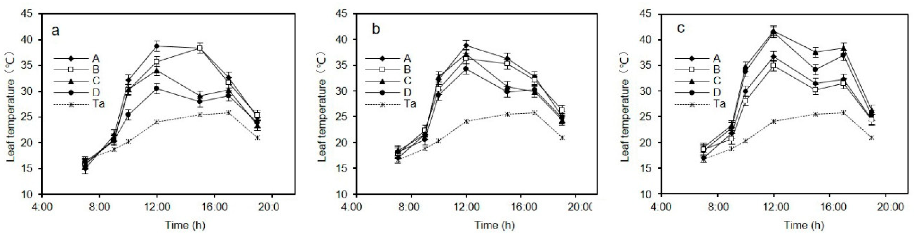
Figure 2.
The relationship between the measured and calculated stomatal conductance values based on the IG (a,c,e) and CWSI (b,d,f) models throughout the experiment. (a,b) are figures of C. korshinskii, (c,d) are of A. ordosica, and (e,f) are of S. psammophila; n > 30.
Figure 2.
The relationship between the measured and calculated stomatal conductance values based on the IG (a,c,e) and CWSI (b,d,f) models throughout the experiment. (a,b) are figures of C. korshinskii, (c,d) are of A. ordosica, and (e,f) are of S. psammophila; n > 30.

Figure 3.
Estimated dependence of gaW and raW on the characteristics of dimension and wind speed for flat leaves (a) and cylindrical leaves (b) in natural environments [6].
Figure 3.
Estimated dependence of gaW and raW on the characteristics of dimension and wind speed for flat leaves (a) and cylindrical leaves (b) in natural environments [6].
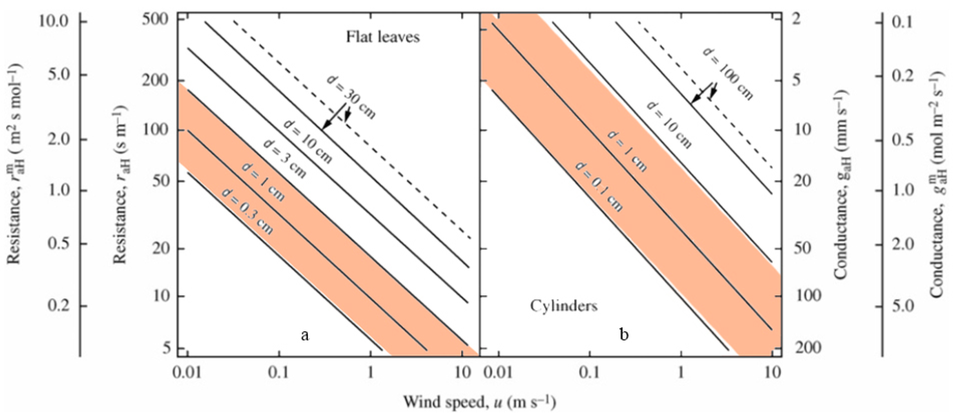
Figure 4.
Daytime stomatal conductance of C. korshinskii (a), A. ordosica (b), and S. psammophila (c) (mean ± SE) under the water deficit gradient (Groups B, C, and D) over a typical day (n = 3 per treatment).
Figure 4.
Daytime stomatal conductance of C. korshinskii (a), A. ordosica (b), and S. psammophila (c) (mean ± SE) under the water deficit gradient (Groups B, C, and D) over a typical day (n = 3 per treatment).
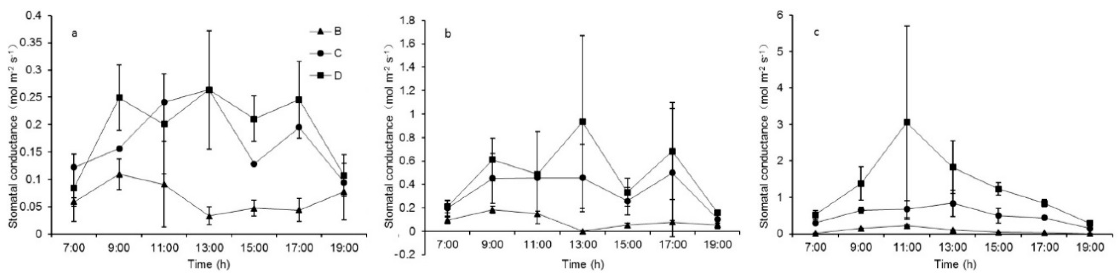
Figure 5.
Leaf shapes of C. korshinskii (a), A. ordosica (b), and S. psammophila (c). The black square in the middle of each image represents 1 × 1 cm.
Figure 5.
Leaf shapes of C. korshinskii (a), A. ordosica (b), and S. psammophila (c). The black square in the middle of each image represents 1 × 1 cm.


Table 1.
Mauchly’s test of sphericity.
| Species | Within Subjects Effect | Mauchly’s W | Approx. Chi-Square | df | Sig. | Epsilona | ||
|---|---|---|---|---|---|---|---|---|
| Greenhouse-Geisser | Huynh-Feldt | Lower-Bound | ||||||
| C. korshinskii | Time | 0.000 | 0.000 | 20 | 0.000 | 0.171 | 0.219 | 0.167 |
| A. ordosica | Time | 0.000 | 0.000 | 20 | 0.000 | 0.177 | 0.229 | 0.167 |
| S. psammophila | Time | 0.000 | 0.000 | 20 | 0.000 | 0.172 | 0.220 | 0.167 |
Table 2.
Tests for within-subject effects on leaf temperature, with Greenhouse-Gersser correction.
| Species | Source | Type III Sum of Squares | df | Mean Square | F | Sig. |
|---|---|---|---|---|---|---|
| C. korshinskii | Time | 7777.755 | 1.028 | 7569.163 | 3132.020 | 0.000 |
| Time * stress gradient | 60.572 | 3.083 | 19.649 | 8.131 | 0.003 | |
| A. ordosica | Time | 7211.525 | 1.065 | 6773.545 | 3047.103 | 0.000 |
| Time * stress gradient | 204.490 | 3.194 | 64.024 | 28.801 | 0.000 | |
| S. psammophila | Time | 7773.256 | 1.030 | 7549.551 | 3105.961 | 0.000 |
| Time * stress gradient | 44.866 | 3.089 | 14.525 | 5.976 | 0.009 |
*: Facter interaction.
Table 3.
Tests for stress gradient effects on leaf temperature.
| Species | Source | Type III Sum of Squares | df | Mean Square | F | Sig. |
|---|---|---|---|---|---|---|
| C. korshinskii | Intercept | 72,860.635 | 1 | 72,860.635 | 3895.984 | 0.000 |
| Stress gradient | 177.694 | 3 | 59.231 | 3.167 | 0.046 | |
| Error | 224.418 | 12 | 18.701 | |||
| A. ordosica | Intercept | 73,069.456 | 1 | 73,069.456 | 3901.886 | 0.000 |
| Stress gradient | 113.097 | 3 | 37.699 | 2.013 | 0.044 | |
| Error | 224.720 | 12 | 18.727 | |||
| S. psammophila | Intercept | 75,321.794 | 1 | 75,321.794 | 3900.677 | 0.000 |
| Stress gradient | 70.266 | 3 | 23.422 | 1.213 | 0.034 | |
| Error | 231.719 | 12 | 19.310 |
Table 4.
Expression of the upper and lower baseline results of the three species.
| Plant Species | Upper Baseline | Lower Baseline |
|---|---|---|
| C. korshinskii | , R2 = 0.3861 | |
| A. ordosica | , R2 = 0.2864 | |
| S. psammophila | , R2 = 0.3599 |
Table 5.
Expression of the CWSI and IG models after parameter calibration.
| Model | Plant Species | Model Expression | R2 |
|---|---|---|---|
| CWSI | C. korshinskii | 0.5052 | |
| A. ordosica | 0.4575 | ||
| S. psammophila | 0.7885 | ||
| IG | C. korshinskii | 0.5214 | |
| A. ordosica | 0.7057 | ||
| S. psammophila | 0.5596 |
R2, determination coefficient.
Table 6.
Model evaluation indices for IG and CWSI.
| Model | Plant Species | a | R2 | RMSE (mol m−2 s−1) | MAE (mol m−2 s−1) | MRE | Ef |
|---|---|---|---|---|---|---|---|
| CWSI | C. korshinskii | 0.86 | 0.09 | 0.23 | 0.19 | 0.50 | 0.43 |
| A. ordosica | 0.85 | 0.41 | 0.48 | 0.39 | 2.00 | 0.63 | |
| S. psammophila | 0.90 | 0.76 | 0.40 | 0.29 | 0.42 | 0.79 | |
| IG | C. korshinskii | 0.95 | 0.34 | 0.21 | 0.18 | 0.60 | 0.58 |
| A. ordosica | 0.94 | 0.51 | 0.45 | 0.37 | 1.09 | 0.59 | |
| S. psammophila | 0.87 | 0.46 | 0.32 | 0.27 | 0.33 | 0.56 |
a: The slopes of the correlation equation between the measured and simulated values; R2, determination coefficient; RMSE, root mean square error of prediction; MAE, mean absolute error; MRE, mean relative error; and, Ef, effectiveness index.
Table 7.
Differences in the stomatal conductance and the leaf temperature between plant species (n = 3 per treatment).
Table 7.
Differences in the stomatal conductance and the leaf temperature between plant species (n = 3 per treatment).
| (a) Leaf Temperature | (b) Stomatal Conductance | ||||||
|---|---|---|---|---|---|---|---|
| Stress Gradient | Mean Square | F | Sig. | Stress Gradient | Mean Square | F | Sig. |
| B | 2.763 | 1.513 | 0.294 | B | 0.006 | 2.417 | 0.195 |
| C | 15.640 | 7.363 | 0.024 | C | 0.592 | 4.019 | 0.078 |
| D | 27.586 | 20.290 | 0.002 | D | 6.715 | 20.803 | 0.002 |
© 2018 by the authors. Licensee MDPI, Basel, Switzerland. This article is an open access article distributed under the terms and conditions of the Creative Commons Attribution (CC BY) license (http://creativecommons.org/licenses/by/4.0/).
Share and Cite
MDPI and ACS Style
Yu, M.; Ding, G.; Gao, G.; Zhao, Y.; Sai, K. Leaf Temperature Fluctuations of Typical Psammophytic Plants and Their Application to Stomatal Conductance Estimation. Forests 2018, 9, 313. https://doi.org/10.3390/f9060313
AMA Style
Yu M, Ding G, Gao G, Zhao Y, Sai K. Leaf Temperature Fluctuations of Typical Psammophytic Plants and Their Application to Stomatal Conductance Estimation. Forests. 2018; 9(6):313. https://doi.org/10.3390/f9060313
Chicago/Turabian StyleYu, Minghan, Guodong Ding, Guanglei Gao, Yuanyuan Zhao, and Ke Sai. 2018. "Leaf Temperature Fluctuations of Typical Psammophytic Plants and Their Application to Stomatal Conductance Estimation" Forests 9, no. 6: 313. https://doi.org/10.3390/f9060313
Note that from the first issue of 2016, this journal uses article numbers instead of page numbers. See further details here.