Article

Spatial Variation in Canopy Structure across Forest Landscapes

by
Brady S. Hardiman
1,2,*,
Elizabeth A. LaRue
1,
Jeff W. Atkins
3,
Robert T. Fahey
4,
Franklin W. Wagner
1 and
Christopher M. Gough
3
1
Department of Forestry & Natural Resources, Purdue University, West Lafayette, IN 47907, USA
2
Department of Ecological and Environmental Engineering, Purdue University, West Lafayette, IN 47907, USA
3
Department of Biology, Virginia Commonwealth University, Richmond, VA 23284, USA
4
Department of Natural Resources and the Environment and Center for Environmental Sciences and Engineering, University of Connecticut, Storrs, CT 06269, USA
*
Author to whom correspondence should be addressed.
Forests 2018, 9(8), 474; https://doi.org/10.3390/f9080474
Submission received: 21 June 2018 / Revised: 30 July 2018 / Accepted: 1 August 2018 / Published: 3 August 2018
(This article belongs to the Special Issue Defining, Quantifying, Observing and Modeling Forest Canopy Traits)

Abstract

:
Forest canopy structure (CS) controls many ecosystem functions and is highly variable across landscapes, but the magnitude and scale of this variation is not well understood. We used a portable canopy LiDAR system to characterize variation in five categories of CS along N = 3 transects (140–800 m long) at each of six forested landscapes within the eastern USA. The cumulative coefficient of variation was calculated for subsegments of each transect to determine the point of stability for individual CS metrics. We then quantified the scale at which CS is autocorrelated using Moran’s I in an Incremental Autocorrelation analysis. All CS metrics reached stable values within 300 m but varied substantially within and among forested landscapes. A stable point of 300 m for CS metrics corresponds with the spatial extent that many ecosystem functions are measured and modeled. Additionally, CS metrics were spatially autocorrelated at 40 to 88 m, suggesting that patch scale disturbance or environmental factors drive these patterns. Our study shows CS is heterogeneous across temperate forest landscapes at the scale of 10 s of meters, requiring a resolution of this size for upscaling CS with remote sensing to large spatial scales.

1. Introduction

In forested ecosystems, the density and spatial arrangement of vegetation, or canopy structure (CS), imposes strong controls on many scale-dependent ecosystem functions. CS in the form of leaf area and arrangement exerts a strong influence on forest production through its effects on light absorption [1] and light-use efficiency [2,3]. CS metrics describing height and heterogeneity affect the turbulent exchange of gases between ecosystems and atmosphere, and regulate canopy net energy balance [4,5,6]. The spatial scale at which canopy structure exerts functionally meaningful effects on ecosystem processes varies depending on forest type and architecture, environmental factors, and the ecosystem functions and the CS element of interest. For example, patterns of light transmittance relate to structure at the scale of individual leaves and small canopy gaps [7], while boundary-layer processes are affected by gaps to landscape-scale canopy structure variations [8]. Inferring and scaling ecosystem functions from remotely sensed measurements of forest structure requires an understanding of how different measures of CS vary spatially across forested landscapes.
CS is an emergent property of multiple underlying ecological factors operating at multiple spatial scales [9,10,11]. Determinants of CS within landscapes may include at the smallest scales the distribution of individual leaves owing to resource availability and at the landscape scale variation in tree mortality and disturbances (Table 1) [12,13]. Additional within-landscape variation is associated with the combined effects of individual-scale tree crown architecture, neighborhood-scale community taxonomic diversity and competition, and environmental variables that shape biomass production and allocation [14,15]. Variation within and among forest stands in these canopy-shaping forces may determine the spatial scale at which CS stabilizes (i.e., spatial extent within a stand at which heterogeneity in CS plateaus), and the degree to which scales of stability differ among forested landscapes [12]. Such understanding of the spatial scales and patterns of variation in CS are essential precursors both to understanding the fundamental drivers of this variation as well as to deriving, interpreting, and modeling ecosystem structure and function across forest stands and landscapes.
Recent methodological advances in LiDAR remote sensing have provided a means to better understand spatial patterns in the variation of forest CS. Terrestrial LiDAR allows for a complete characterization of the arrangement of vegetation throughout the entire canopy volume [16,17] with a level of detail not possible from aerial or satellite forms of LiDAR [18]. Therefore, to advance our understanding of the patterns in variation of forest CS, we chose to use terrestrial LiDAR to examine and compare variation in landscape-scale CS of mature temperate forests in the northeastern, Great Lakes, and prairie peninsula ecoclimatic domains of the USA (see Thorpe [19] for NEON domains). We used terrestrial LiDAR to measure CS, which provides high-resolution spatially continuous canopy structure data quantitatively describing vegetation density, arrangement, and heterogeneity [20]. Our primary objective was to identify the magnitude of variation and spatial scale of stability in CS within these forested landscapes. We focused on mature temperate forests to evaluate whether these similarly-aged secondary forests located in the northern continental USA exhibit similar spatial scales of CS stability.

2. Materials and Methods

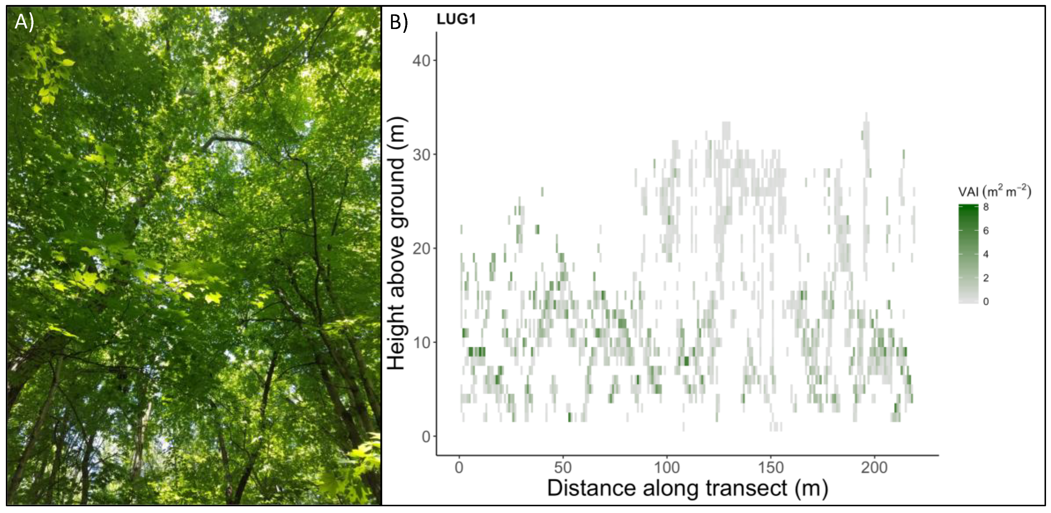
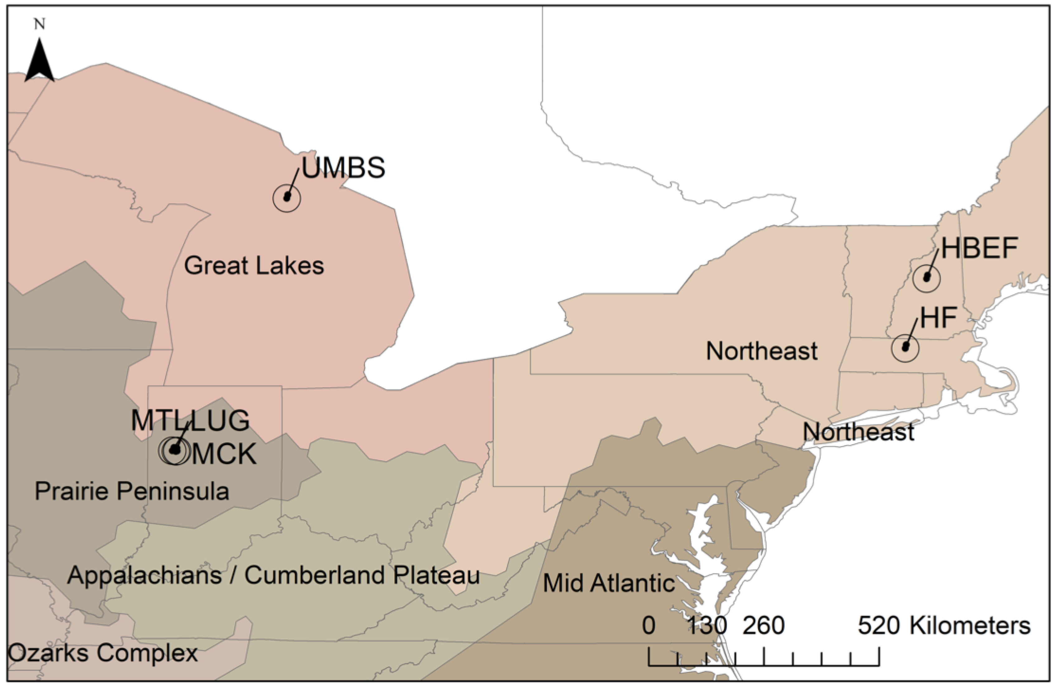
2.1. Portable Canopy LiDAR and Forest Landscapes

We used a portable canopy LiDAR (PCL) system, a type of terrestrial LiDAR to survey CS along a vertical cross section of canopy. The portable canopy LiDAR system contains an upward facing, near-infrared (0.9 μm) pulsed laser operating at 2000 Hz (Riegl LD90 3100 VHS; Riegl USA Inc., Orlando, FL, USA) that is mounted to a frame worn by a user and operated along a transect at a constant speed. The design and operation of the instrument is outlined in Parker et al. [44]. Laser pulses emitted by the LiDAR unit either reflect off objects in the forest canopy or, when a gap is encountered, are not returned. These reflected and un-reflected pulses are recorded and used to construct a vertical cross-section of forest canopy. These “hit-grid” data (Figure 1) are then used to calculate metrics of CS [2].
We collected PCL data from six deciduous forested landscapes in Eastern North America (Figure 2). Five of the six landscapes were characterized by a deciduous, mixed hardwoods species composition, while Harvard Forest (HF) was composed primarily of eastern hemlock (Tsuga Canadensis L.). Within each landscape, we collected PCL data from N = 3 transects (140–800 m; see Figure S1 for individual transect lengths). We sampled within contiguous forest landscapes and thus sampling lengths varied among forested landscapes depending on the dimensions and area of each. Sampling after leaf-out occurred during May 2018 in Indiana locations at McCormick Creek (MCK), Lugar Farm (LUG), and Martell Forest (MTL); August 2017 at Harvard Forest (HF); during summer 2016 at the University of Michigan Biological Station; and August 2017 at Hubbard Brook Experimental Forest (HBEF). Management and disturbance are important sources of variation in canopy structure at a variety of scales. We attempted to minimize these effects by restricting transect length such that each transect fit within a single forest patch with a common management/disturbance history. Within each site, we select patches with similar composition and management/disturbance history and attempted to avoid transects that crossed ecotones or other obvious ecological gradients.

2.2. Canopy Structural Complexity

We focused our analysis on five metrics of CS broadly demonstrated to be functionally important, particularly with respect to canopy light interception and carbon uptake [1]. These metrics fall within five different CS categories: (1) vegetation height (mean maximum outer canopy height, MOCH); (2) vegetation density, volume, and area (mean vegetation area index, VAI); (3) arrangement and distribution (canopy rugosity, RC); (4) cover and openness (gap fraction, GF); and (5) vegetation variability (porosity, PC) [20]. The detailed definitions, derivation, and calculation of each of the five metrics are available in Atkins et al. [20] and in Table S1. The raw PCL data were processed using the forestr package [20], available in R 3.4.4 [45].

2.3. Statistical Analyses
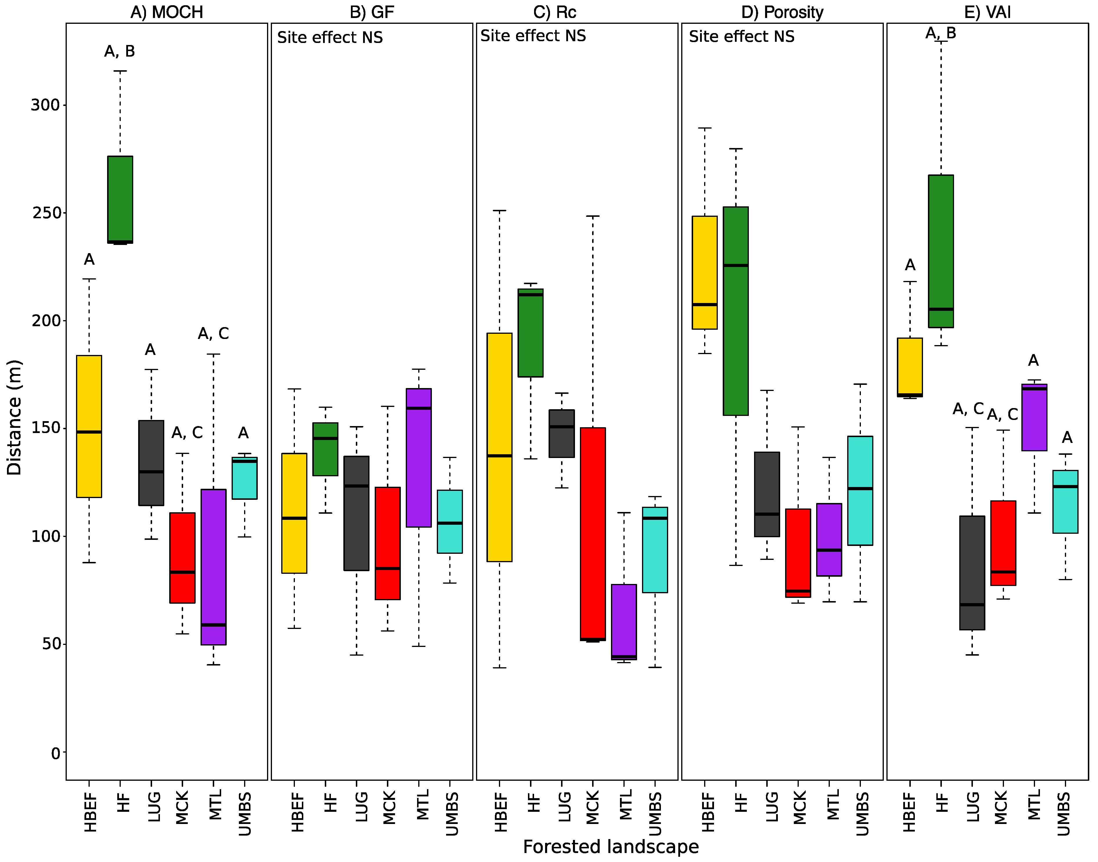
Our first analysis identified the sampling distance at which CS metrics stabilized within each sampled forested landscape. Changes with sampling distance in the coefficient of variation (CV) of each CS metric was derived from cumulative 10-m means and variances across each transect (i.e., 0–10, 0–20, 0–30,… up to the maximum transect length, varying from 140–800 m). The distances at which additional canopy structural information no longer significantly shifts in variance, hereafter termed “stability points,” were estimated from Bayesian changepoint analysis using the bcp package [46] in R 3.4.4 [45]. The distance at which stability in the CV of CS metrics occurred was recorded using both methods (cumulative CV and Bayesian changepoint) and then averaged for a conservative transect level measure of stability distance. We tested for differences in the mean stability point among forested landscapes for each CS metric with one-way ANOVAs. Stability points for RC did not meet the assumption of normality. Therefore, we used a Kruskal-Wallis test to assess differences in mean stability points among forested landscapes. If the landscape effect was not significant, we calculated a mean stability point across forested landscape. If the effect was statistically significant, then we conducted post hoc Tukey tests to compare stability points among forested landscapes.
We conducted a second analysis using Incremental Autocorrelation analysis to assess spatial clustering patterns among CS metrics and across forested landscapes. For each forested landscape and CS metric combination we calculated Moran’s I for all points separated by a given distance as a measure of autocorrelation by distance. We calculated the level of I at 10 m distance increments for the full range of possible sampling distances, starting at 10 m and ending at 150 (LUG, UMBS) or 200 m (all other sites). For each distance increment the z-score and p-value associated with the Moran’s I test statistic were calculated and then z-scores were compared across distances. The distance (or distances) at which the z-score peaked was determined from the data and utilized as an indicator of spatial clustering for each metric and site combination. Incremental Autocorrelation analysis was conducted using the Spatial Analyst toolbox in ArcGIS v. 10.3 (ESRI; Redlands, CA, USA).

3. Results

3.1. Transect Lengths at Which CS Metrics Stabilize

The stability points for two of the five CS metrics differed significantly among forested landscapes. Significant differences were observed among forested landscapes in the distance at which variation (i.e., as CV) in mean outer canopy height (Figure 3A) and VAI (Figure 3E) stabilized. Specifically, the stability point of mean outer canopy height for HF (262 m) was significantly greater than that of MLT (94 m) and MCK (92 m) (Figure 3A). Additionally, the stability point for VAI at HF (241 m) was greater than that of LUG (87 m) and MCK (101 m). However, there were no significant differences in stability points among forested sites for gap fraction (Figure 3B), canopy rugosity (Figure 3C), or porosity (Figure 3D). Average stability points among forested landscapes for gap fraction, canopy rugosity, and porosity were 115 m, 125 m, and 144 m, respectively. All CS metrics exhibited a tendency to converge toward similar values at sufficiently long transect lengths (~300 m), regardless of site (Figure S1). Stability points were not consistently related to the value of each CS metric across sites, except in the case of porosity (Figure S2). At all sites, running means of CV calculated for each CS metric exhibited lower variability when calculated at longer transect lengths (Figures S3–S6).

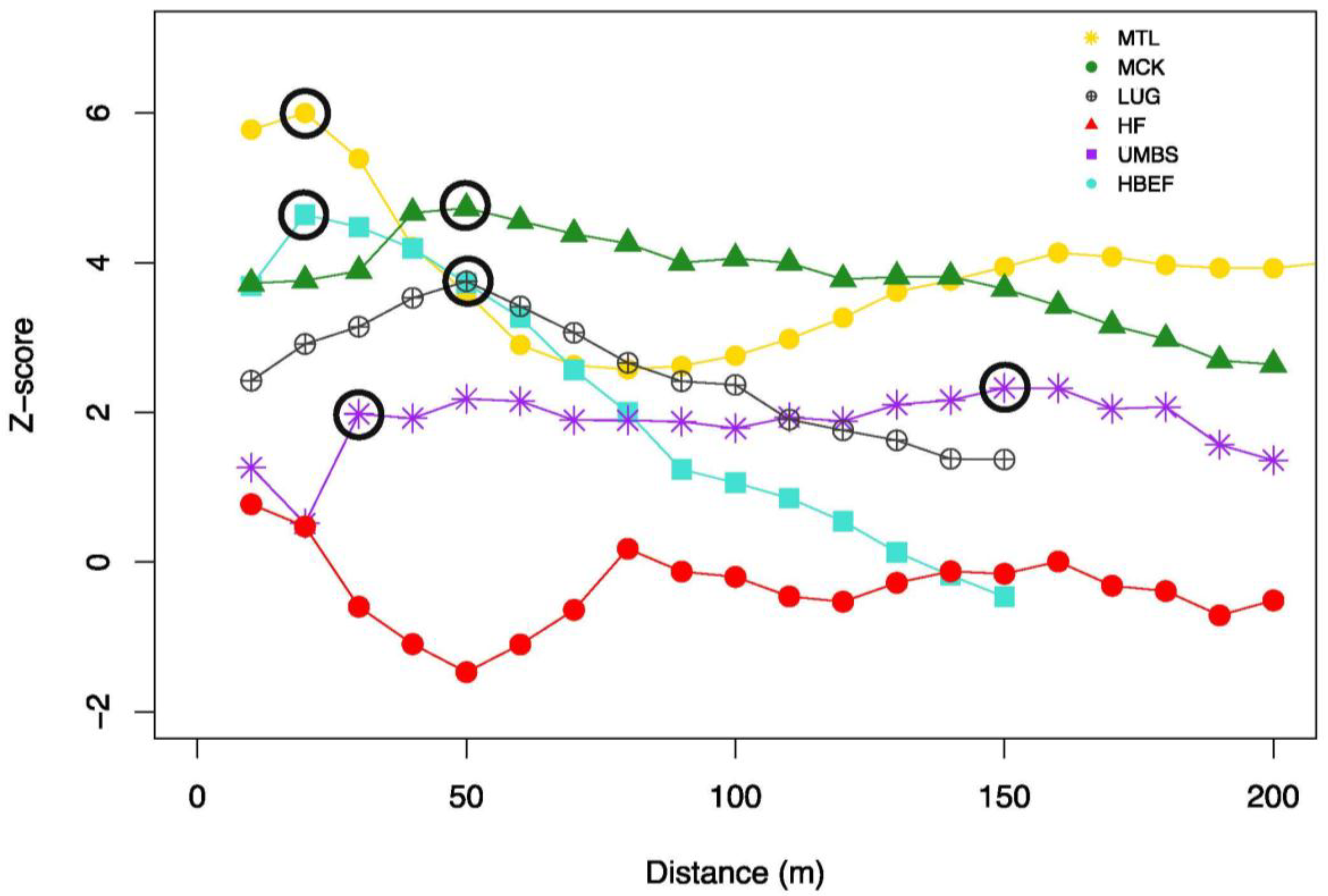
3.2. Scales of Canopy Structure Autocorrelation

Peak spatial autocorrelation along transects varied among CS metrics and forested landscapes. Mean peak spatial autocorrelation distances of the five CS metrics varied substantially among CS metrics, ranging from 40 to 88 m (Table 2). Mean outer canopy height, VAI, and canopy rugosity displayed peak spatial autocorrelation at shorter distances than gap fraction and porosity (Table 2). While among forested landscapes, peak distances of spatial autocorrelation in CS metrics were highly variable, from 20 to 180 m (Table 2). For example, peak spatial autocorrelation of canopy rugosity ranged among landscapes from 20 to 150 m (mean = 53 m; Figure 4), with MTL significantly peaking at both 30 and 150 m (Figure 4). Similarly, VAI and porosity of MCK and mean outer canopy height of MTL exhibited peak autocorrelation at multiple distances, indicating correspondence of VAI at multiple spatial scales. Deep gap fraction, which was zero along many 10 m transect subsegments, displayed significant peak autocorrelation distances in only two of six forested landscapes. One forested landscape, UMBS, exhibited a statistically significant peak distance of autocorrelation for porosity and canopy, but not for the other three CS metrics. Overall, peak autocorrelation when it occurred, varied substantially among forested landscapes for different CS metrics.

4. Discussion

4.1. Spatial Variation and Autocorrelation of Canopy Structure

CS varied substantially across spatial scales both within and among forest landscapes but, despite this variation, all CS metrics reached stable values within 300 m. The distance at which CS stabilized varied substantially among forested landscapes, with midwestern sites generally achieved stability at shorter distances, suggesting greater structural homogeneity, than eastern sites. Among CS metrics, mean outer canopy height and VAI varied significantly among forested landscapes, while gap fraction, canopy rugosity, and porosity did not. Even so, all CS parameters and sites reached stability between 50 to 300 m indicating geographically and biologically distinct forested landscapes, and different measures of CS, reach stability at similar spatial scales of tens to hundreds of meters. This broad convergence of stability within 300 m shows that different structural measures within various landscapes align with many fundamental ecosystem functions that operate and are measured and modeled at similar spatial scales, including net ecosystem production and evapotranspiration [4,47,48].
The spatial scale of CS autocorrelation suggests that the drivers creating this structure are likely to be local disturbance patterns or environmental quality. The mean spatial autocorrelation across forested landscapes ranged between 40–88 m. This local scale of spatial autocorrelation reveals the potential for landscape patterns of patchiness in CS features to emerge, with differences among landscapes occurring [49]. Such differences among metrics in spatial clustering likely reflect the underlying ecological drivers of each structural measure such as the variety in crown architecture and disturbance history in the specific forests that were sampled. For example, the CS metric with the shortest peak distance was gap fraction, which likely reflects the ubiquitous distribution of small gaps in the mature forest examined [50,51,52]. Likewise, VAI had the longest distance of peak autocorrelation, likely reflecting spatial differentiation within landscapes as a function of variable soil fertility and management history. For some CS metrics we observed a high degree of consistency across most or all forested landscapes (GF, Porosity, VAI) suggesting a common driver of these metrics, while the other metrics may be driven primarily by forest stand–specific factors such as recent disturbances. Indeed, forests at HF and HBEF have recently experienced well documented disruptions to CS prompted by widespread tree mortality [32,53,54]. Accounting for this spatial autocorrelation in the design of a sampling plan can improve the robustness of studies that rely on the characterization of CS across space [55]. Our study clearly sheds light on the need to understand spatial scales of autocorrelation in CS because the potential for patchiness in CS within and across landscapes will influence design of robust empirical studies and strategies for modeling forest processes.
While approaches to describing CS with LiDAR have become increasingly sophisticated, no single LiDAR technology (aerial, terrestrial) can perfectly capture all aspects of forest canopies—occlusion of canopy elements remains a challenge for all LiDAR applications. Terrestrial and aerial LiDAR suffer equally from this issue but combining them offers the potential to minimize the portion of the canopy that is obscured. Improving understanding of how CS varies across spatial scales within stands, across landscapes, and among forest types requires coupling of terrestrial and aerial LiDAR [56,57] and will, increasingly, involve integration of LiDAR mounted on unoccupied aerial vehicles (UAVs). Our study shows that the spatial scale of stability in CS may be best characterized by terrestrial LiDAR and then scaled up to a larger footprint with aerial LiDAR. Terrestrial LiDAR platforms provide an advantage over downward looking aerial LiDAR [18] by providing a characterization of the arrangement of internal canopy elements that are difficult to detect with aerial LiDAR due to occlusion and lower point density. CS metrics from terrestrial LiDAR have proven to have high value in describing structures that are important to ecosystem functioning [1,58]. Similar information could be extracted from aerial LiDAR data, especially from full waveform or Geiger-mode platforms, but the correct scale at which to describe such CS metrics (which has generally been constrained in terrestrial LiDAR studies by sampling schemes) is not well understood. Recent studies have documented the substantial influence of CS, as measured by TLS, on remote sensing observations of forests (e.g., Landsat; [59]), demonstrating potential new methods to derive additional information from existing data streams. However, despite these linkages, the spatial coherence of terrestrial and aerial measures of structure is uncertain due to differences in the scale of measurement. Coupling the two will require understanding the scales of CS variation within contiguous areas of forestland.

4.2. Relevance to Canopy Structural Scaling and Modelling Efforts

Our results suggest that surveys of CS are likely to correspond well with functions examined at a “foot-print” scale. For example, the maximum stability point of 300 m corresponds with the area of measurements of forest carbon exchange by eddy covariance towers [4,47]. Analysis of stability points and autocorrelation scales for CS metrics indicate that CS can be robustly estimated and upscaled within an area of observation typical of that already employed by many forest ecological studies. While all metrics achieved stability within 300 m, some categories of CS metrics do appear inherently more spatially variable regardless of landscape (Figure 3), suggesting that upscaling some metrics may necessitate coarser resolution of outputs. Given the spatial variation in stability points and auto-correlation across forest landscapes and parameters, scaling and modeling of CS requires a nuanced approach. Our analysis indicates that, while CS is stable within landscapes, it tends to shift across landscapes, suggesting that scaling of contiguous landscape units may be important.
Improved characterization of spatial variation of CS has several potential benefits for understanding and modelling scale-dependent forest ecosystem processes. First, ecosystem models greatly simplify complex CS to improve computational tractability [60]. While computational tractability is desirable, output from such models often fails to accurately describe forest process and responses to disturbance. More accurate representation of CS could improve model performance by increasing biological realism. Second, many ecosystem models accommodate some degree of vertical variation in vegetation distribution, but most do not explicitly incorporate horizontal heterogeneity in vertical variation, limiting their ability to accurately represent spatially heterogeneous processes such as disturbance events which are known to influence CS and functions such as carbon cycling [26,29]. Third, incorporating CS and the spatial variation thereof in ecosystem models offers opportunities to represent disturbance and successional changes through their effects on CS itself rather than by attempting to capture and represent the mechanism of disturbance itself.

5. Conclusions

We conclude that, although CS metrics stabilize within forested landscapes at different spatial scales, all approach stability at distances under 300 m. This is a range that is well aligned with the spatial scale at which many fundamental ecosystem functions are quantified using measurements and models. This finding has important implications for remote sensing, upscaling, and modeling of CS and functions inferred from or influenced by structure. New remote sensing platforms, such as terrestrial LiDAR, are increasingly available and are likely to become a common component of the forest ecology toolkit in the near future. The data generated by these tools will help to answer ecological questions requiring a rigorous understanding of the scales at which CS vary across the landscape. Furthermore, there are likely to be many drivers of landscape variation in canopy structure; future research should investigate the underlying causes of variation in CS across and within spatial scales.

Supplementary Materials

The following are available online at https://www.mdpi.com/1999-4907/9/8/474/s1, Table S1. Definitions of canopy structure metrics employed in this analysis. Figure S1. Coefficient of variation of canopy structural complexity metrics from n = 3 individual transects at each of six forested landscapes in Eastern North America. Figure S2. Univariate regression analysis between canopy structure metrics and stability points of CS metrics from Bayesian changepoint analysis along forested transects from six forested landscapes in eastern USA. Figure S3. Variation in the value of CS metrics calculated at a range of scales at Harvard Forest. Figure S4. Variation in the value of CS metrics calculated at a range of scales at Martell Forest. Figure S5. Variation in the value of CS metrics calculated at a range of scales at University of Michigan Biological Station (UMBS). Figure S6. Variation in the value of CS metrics calculated at a range of scales at Hubbard Brook Experimental Forest.

Author Contributions

Conceptualization, B.S.H. and J.W.A.; Data curation, J.W.A. and F.W.W.; Formal analysis, E.A.L., J.W.A. and R.T.F.; Funding acquisition, B.S.H., R.T.F., and C.M.G.; Methodology, E.A.L., J.W.A., R.T.F. and F.W.W.; Project administration, B.S.H., R.T.F. and C.M.G.; Resources, B.S.H. and C.M.G.; Supervision, B.S.H.; Visualization, E.A.L. and J.W.A.; Writing—original draft, B.S.H., E.A.L., J.W.A., R.T.F., and C.M.G.; Writing—review and editing, B.S.H., E.A.L., J.W.A., R.T.F., and C.M.G.

Funding

This research was funded by the National Science Foundation’s Division of Emerging Frontiers, EAGER-NEON Awards 1550657 (to CMG), 1550650 (to RTF), and 1550639 (to BSH). CMG and JWA were additionally supported by National Science Foundation Award 1655095. EAL was supported in part by NSF Division of Emerging Frontiers Award 1638702 (to BSH).

Acknowledgments

We acknowledge the contributions of Michael Keller, Nathan Ibarluzea, Ke Xu, and Emily Summers who assisted with data collection at the Purdue University sites, as well as Nat Cleavitt and Jackie Hatala-Matthes for assistance with data collection at Hubbard Brook Experimental Forest. We thank staff from the University of Michigan Biological Station, Harvard Forest, Hubbard Brook Experimental Forest, and Purdue University Department of Forestry and Natural Resources for material support.

Conflicts of Interest

The authors declare no conflict of interest.

References

  1. Atkins, J.W.; Fahey, R.T.; Hardiman, B.S.; Gough, C.M. Forest Canopy Structural Complexity and light absorption relationships at the subcontinental scale. J. Geophys. Res. Biogeosci. 2018, 123, 1387–1405. [Google Scholar] [CrossRef]
  2. Hardiman, B.S.; Bohrer, G.; Gough, C.M.; Vogel, C.S.; Curtis, P.S. The role of canopy structural complexity in wood net primary production of a maturing northern deciduous forest. Ecology 2011, 92, 1818–1827. [Google Scholar] [CrossRef] [PubMed]
  3. Hardiman, B.S.; Gough, C.M.; Halperin, A.; Hofmeister, K.L.; Nave, L.E.; Bohrer, G.; Curtis, P.S. Maintaining high rates of carbon storage in old forests: A mechanism linking canopy structure to forest function. For. Ecol. Manag. 2013, 298, 111–119. [Google Scholar] [CrossRef]
  4. Maurer, K.D.; Hardiman, B.S.; Vogel, C.S.; Bohrer, G. Canopy-structure effects on surface roughness parameters: Observations in a great lakes mixed-deciduous forest. Agric. For. Meteorol. 2013, 177, 24–34. [Google Scholar] [CrossRef]
  5. Bonan, G.B. Forests and climate change: Forcings, feedbacks, and the climate benefits of forests. Science 2008, 320, 1444–1449. [Google Scholar] [CrossRef] [PubMed]
  6. Yang, R.; Friedl, M.A. Modeling the effects of three-dimensional vegetation structure on surface radiation and energy balance in boreal forests. J. Geophys. Res. 2003, 108, 8615. [Google Scholar] [CrossRef]
  7. Ellsworth, D.S.; Reich, P.B. Canopy structure and vertical patterns of photosynthesis and related leaf traits in a deciduous forest. Oecologia 1993, 96, 169–178. [Google Scholar] [CrossRef] [PubMed]
  8. Yang, R.; Friedl, M.A. Determination of roughness lengths for heat and momentum over boreal forests. Bound.-Layer Meteorol. 2003, 107, 581–603. [Google Scholar] [CrossRef]
  9. Aber, J.D.; Pastor, J.; Melillo, J.M. Changes in forest canopy structure along a site quality gradient in southern Wisconsin, USA. Am. Midl. Nat. 1982, 108, 256–265. [Google Scholar] [CrossRef]
  10. Parker, G.G.; Russ, M.E. The canopy surface and stand development: Assessing forest canopy structure and complexity with near-surface altimetry. For. Ecol. Manag. 2004, 189, 307–315. [Google Scholar] [CrossRef]
  11. Hutchison, B.A.; Matt, D.R.; Mcmillen, R.T.; Gross, L.J.; Tajchman, S.J.; Norman, J.M. The architecture of a deciduous forest canopy in eastern Tennessee, USA. J. Ecol. 1986, 74, 635–646. [Google Scholar] [CrossRef]
  12. Nadkarni, N.M.; McIntosh, A.C.S.; Cushing, J.B. A framework to categorize forest structure concepts. For. Ecol. Manag. 2008, 256, 872–882. [Google Scholar] [CrossRef] [Green Version]
  13. Kane, V.R.; Bakker, J.D.; McGaughey, R.J.; Lutz, J.A.; Gersonde, R.F.; Franklin, J.F. Examining conifer canopy structural complexity across forest ages and elevations with LiDAR data. Can. J. For. Res. Can. Res. 2010, 40, 774–787. [Google Scholar] [CrossRef] [Green Version]
  14. Ishii, H.T.; Tanabe, S.; Hiura, T. Exploring the relationships among canopy structure, stand productivity, and biodiversity of temperature forest ecosystems. For. Sci. 2004, 50, 342–355. [Google Scholar]
  15. Lefsky, M.A.; Hudak, A.T.; Cohen, W.B.; Acker, S.A. Geographic variability in lidar predictions of forest stand structure in the Pacific Northwest. Remote Sens. Environ. 2005, 95, 532–548. [Google Scholar] [CrossRef]
  16. Paynter, I.; Saenz, E.; Genest, D.; Peri, F.; Erb, A.; Li, Z.; Wiggin, K.; Muir, J.; Raumonen, P.; Schaaf, E.S.; et al. Observing ecosystems with lightweight, rapid-scanning terrestrial lidar scanners. Remote Sens. Ecol. Conserv. 2016, 2, 174–189. [Google Scholar] [CrossRef] [Green Version]
  17. Newnham, G.J.; Armston, J.D.; Calders, K.; Disney, M.I.; Lovell, J.L.; Schaaf, C.B.; Strahler, A.H.; Danson, F.M. Terrestrial laser scanning for plot-scale forest measurement. Curr. For. Rep. 2015, 1, 239–251. [Google Scholar] [CrossRef]
  18. Kükenbrink, D.; Schneider, F.D.; Leiterer, R.; Schaepman, M.E.; Morsdorf, F. Quantification of hidden canopy volume of airborne laser scanning data using a voxel traversal algorithm. Remote Sens. Environ. 2017, 194, 424–436. [Google Scholar] [CrossRef]
  19. Thorpe, A.S.; Barnett, D.T.; Elmendorf, S.C.; Hinckley, E.L.S.; Hoekman, D.; Jones, K.D.; Levan, K.E.; Meier, C.L.; Stanish, L.F.; Thibault, K.M. Introduction to the sampling designs of the national ecological observatory network terrestrial observation system. Ecosphere 2016, 7, 1–11. [Google Scholar] [CrossRef]
  20. Atkins, J.; Bohrer, G.; Fahey, R.; Hardiman, B.; Morin, T.; Stovall, A.; Zimmerman, N.; Gough, C. Quantifying forest and canopy structural complexity metrics from terrestrial LiDAR data using the forestr R package. Methods Ecol. Evol. 2018, in press. [Google Scholar] [CrossRef]
  21. Niinemets, Ü. Photosynthesis and resource distribution through plant canopies. Plant Cell Environ. 2007, 30, 1052–1071. [Google Scholar] [CrossRef] [PubMed] [Green Version]
  22. Mori, A.; Niinemets, Ü. Plant responses to heterogeneous environments: Scaling from shoot modules and whole-plant functions to ecosystem processes. Ecol. Res. 2010, 25, 691–692. [Google Scholar] [CrossRef]
  23. Niinemets, Ü. A review of light interception in plant stands from leaf to canopy in different plant functional types and in species with varying shade tolerance. Ecol. Res. 2010, 25, 671–693. [Google Scholar] [CrossRef]
  24. Ishii, H.; Asano, S. The role of crown architecture, leaf phenology and photosynthetic activity in promoting complementary use of light among coexisting species in temperate forests. Ecol. Res. 2009, 25, 715–722. [Google Scholar] [CrossRef]
  25. Pretzsch, H.; Forrester, D.I.; Rötzer, T. Representation of species mixing in forest growth models: A review and perspective. Ecol. Model. 2015, 313, 276–292. [Google Scholar] [CrossRef]
  26. Curtis, P.S.; Gough, C.M. Forest aging, disturbance and the carbon cycle. New Phytol. 2018, in press. [Google Scholar] [CrossRef] [PubMed]
  27. Franklin, J. Disturbances and structural development of natural forest ecosystems with silvicultural implications, using Douglas-fir forests as an example. For. Ecol. Manag. 2002, 155, 399–423. [Google Scholar] [CrossRef]
  28. Fotis, A.T.; Morin, T.H.; Fahey, R.T.; Hardiman, B.S.; Bohrer, G.; Curtis, P.S. Forest structure in space and time: Biotic and abiotic determinants of canopy complexity and their effects on net primary productivity. Agric. For. Meteorol. 2018, 250–251, 181–191. [Google Scholar] [CrossRef]
  29. Sagara, B.T.; Fahey, R.T.; Vogel, C.S.; Fotis, A.T.; Curtis, P.S.; Gough, C.M. Moderate disturbance has similar effects on production regardless of site quality and composition. Forests 2018, 9, 70. [Google Scholar] [CrossRef]
  30. Tanaka, H.; Nakashizuka, T. Fifteen years of canopy dynamics analyzed by aerial photographs in a temperate deciduous forest, Japan. Ecology 1997, 78, 612–620. [Google Scholar] [CrossRef]
  31. Hardiman, B.S.; Bohrer, G.; Gough, C.M.; Curtis, P.S. Canopy structural changes following widespread mortality of canopy dominant trees. Forests 2013, 4, 537–552. [Google Scholar] [CrossRef]
  32. Pederson, N.; Dyer, J.M.; Mcewan, R.W.; Hessl, A.E.; Mock, C.J.; Orwig, D.A.; Rieder, H.E.; Cook, B.I. The legacy of episodic climatic events in shaping temperate, broadleaf forests. Ecol. Monogr. 2014, 84, 599–620. [Google Scholar] [CrossRef]
  33. Fahey, R.T.; Alveshere, B.C.; Burton, J.I.; D’Amato, A.W.; Dickinson, Y.L.; Keeton, W.S.; Kern, C.C.; Larson, A.J.; Palik, B.J.; Puettmann, K.J.; et al. Shifting conceptions of complexity in forest management and silviculture. For. Ecol. Manag. 2018, 421, 59–71. [Google Scholar] [CrossRef]
  34. Hiroaki, T.; Van Pelt, R.; Parker, G.; Nadkarni, N. Age-related development of canopy structure and its ecological functions. In Forest Canopies; Lowman, M., Rinker, H., Eds.; Elsevier Academic Press: Amsterdam, The Netherlands, 2004; pp. 102–117. [Google Scholar]
  35. Fahey, R.T.; Fotis, A.T.; Woods, K.D. Quantifying canopy complexity and effects on productivity and resilience in late-successional hemlock-hardwood forests. Ecol. Appl. 2015, 25, 834–847. [Google Scholar] [CrossRef] [PubMed]
  36. McMahon, S.M.; Parker, G.G.; Miller, D.R. Evidence for a recent increase in forest growth. Proc. Natl. Acad. Sci. USA 2010, 107, 3611–3615. [Google Scholar] [CrossRef] [PubMed] [Green Version]
  37. Montgomery, R.A.; Chazdon, R.L. Forest structure, canopy architecture, and light transmittance in tropical wet forests. Ecology 2001, 82, 2707–2718. [Google Scholar] [CrossRef]
  38. McMahon, S.M.; Bebber, D.P.; Butt, N.; Crockatt, M.; Kirby, K.; Parker, G.G.; Riutta, T.; Slade, E.M. Ground based LiDAR demonstrates the legacy of management history to canopy structure and composition across a fragmented temperate woodland. For. Ecol. Manag. 2015, 335, 255–260. [Google Scholar] [CrossRef]
  39. Nave, L.E.; Sparks, J.P.; Le Moine, J.; Hardiman, B.S.; Nadelhoffer, K.J.; Tallant, J.M.; Vogel, C.S.; Strahm, B.D.; Curtis, P.S. Changes in soil nitrogen cycling in a northern temperate forest ecosystem during succession. Biogeochemistry 2014, 3, 471–488. [Google Scholar] [CrossRef]
  40. Morton, D.C.; Nagol, J.; Carabajal, C.C.; Rosette, J.; Palace, M.; Cook, B.D.; Vermote, E.F.; Harding, D.J.; North, P.R.J. Amazon forests maintain consistent canopy structure and greenness during the dry season. Nature 2014, 506, 1–16. [Google Scholar] [CrossRef] [PubMed]
  41. Saatchi, S.; Marlier, M.; Chazdon, R.L.; Clark, D.B.; Russell, A.E. Impact of spatial variability of tropical forest structure on radar estimation of aboveground biomass. Remote Sens. Environ. 2011, 115, 2836–2849. [Google Scholar] [CrossRef]
  42. Saatchi, S.; Asefi-Najafabady, S.; Malhi, Y.; Aragao, L.E.O.C.; Anderson, L.O.; Myneni, R.B.; Nemani, R. Persistent effects of a severe drought on Amazonian forest canopy. Proc. Natl. Acad. Sci. USA 2013, 110, 565–570. [Google Scholar] [CrossRef] [PubMed]
  43. Wirth, R.; Weber, B.; Ryel, R.J. Spatial and temporal variability of canopy structure in a tropical moist forest. Acta Oecol. 2001, 22, 235–244. [Google Scholar] [CrossRef]
  44. Parker, G.G.; Harding, D.J.; Berger, M.L. A portable LIDAR system for rapid determination of forest canopy structure. J. Appl. Ecol. 2004, 41, 755–767. [Google Scholar] [CrossRef] [Green Version]
  45. Schmid, H.P.; Su, H.B.; Vogel, C.S.; Curtis, P.S. Ecosystem-atmosphere exchange of carbon dioxide over a mixed hardwood forest in northern lower Michigan. J. Geophys. Res. 2003, 108, 19. [Google Scholar] [CrossRef]
  46. Kane, V.R.; Gersonde, R.F.; Lutz, J.A.; McGaughey, R.J.; Bakker, J.D.; Franklin, J.F. Patch dynamics and the development of structural and spatial heterogeneity in Pacific Northwest forests. Can. J. For. Res. 2011, 41, 2276–2291. [Google Scholar] [CrossRef]
  47. Miller, T.F.; Mladenoff, D.J.; Clayton, M.K. Old-growth northern hardwood forests: Spatial autocorrelation and pattern of understory vegetation. Ecol. Monogr. 2002, 72, 487–503. [Google Scholar] [CrossRef]
  48. Runkle, J.R. Gap regeneration in some old-growth forests of the Eastern-United-States. Ecology 1981, 62, 1041–1051. [Google Scholar] [CrossRef]
  49. Runkle, J.R.; Yetter, T.C. Treefalls revisited: Gap dynamics in the southern appalachians. Ecology 1987, 68, 417–424. [Google Scholar] [CrossRef]
  50. Hibbs, D.E. Gap Dynamics in A Hemlock Hardwood Forest. Can. J. For. Res. Can. Rech. For. 1982, 12, 522–527. [Google Scholar] [CrossRef]
  51. Orwig, D.A.; Cobb, R.C.; D’Amato, A.W.; Kizlinski, M.L.; Foster, D.R. Multi-year ecosystem response to hemlock woolly adelgid infestation in southern New England forests. Can. J. For. Res. Can. Rech. For. 2008, 38, 834–843. [Google Scholar] [CrossRef]
  52. Orwig, D.A.; Barker Plotkin, A.A.; Davidson, E.A.; Lux, H.; Savage, K.E.; Ellison, A.M. Foundation species loss affects vegetation structure more than ecosystem function in a northeastern USA forest. Peer J. 2013, 1, e41. [Google Scholar] [CrossRef] [PubMed] [Green Version]
  53. Pickell, P.D.; Coops, N.C.; Gergel, S.E.; Andison, D.W.; Marshall, P.L. Evolution of Canada’s boreal forest spatial patterns as seen from space. PLoS ONE 2016, 11, e0157736. [Google Scholar] [CrossRef] [PubMed]
  54. Schneider, F.D.; Leiterer, R.; Morsdorf, F.; Gastellu-Etchegorry, J.P.; Lauret, N.; Pfeifer, N.; Schaepman, M.E. Simulating imaging spectrometer data: 3D forest modeling based on LiDAR and in situ data. Remote Sens. Environ. 2014, 152, 235–250. [Google Scholar] [CrossRef]
  55. Moran, C.J.; Rowell, E.M.; Seielstad, C.A. A data-driven framework to identify and compare forest structure classes using LiDAR. Remote Sens. Environ. 2018, 211, 154–166. [Google Scholar] [CrossRef]
  56. Ehbrecht, M.; Schall, P.; Ammer, C.; Seidel, D. Quantifying stand structural complexity and its relationship with forest management, tree species diversity and microclimate. Agric. For. Meteorol. 2017, 242, 1–9. [Google Scholar] [CrossRef]
  57. LaRue, E.; Atkins, J.; Dahlin, K.; Fahey, R.; Fei, S.; Gough, C.; Hardiman, B. Linking Landsat to terrestrial LiDAR: Vegetation metrics of forest greenness are correlated with canopy structural complexity. Int. J. Appl. Earth Obs. Geoinf. 2018, 73, 420–427. [Google Scholar] [CrossRef]
  58. Mahadevan, P.; Wofsy, S.C.; Matross, D.M.; Xiao, X.; Dunn, A.L.; Lin, J.C.; Gerbig, C.; Munger, J.W.; Chow, V.Y.; Gottlieb, E.W. A satellite-based biosphere parameterization for net ecosystem CO2 exchange: Vegetation photosynthesis and respiration model (VPRM). Glob. Biogeochem. Cycles 2008, 22. [Google Scholar] [CrossRef]
  59. Medvigy, D.; Wofsy, S.C.; Munger, J.W.; Hollinger, D.Y.; Moorcroft, P.R. Mechanistic scaling of ecosystem function and dynamics in space and time: Ecosystem demography model version 2. J. Geophys. Res. 2009, 114, 1–21. [Google Scholar] [CrossRef]
  60. Bond-Lamberty, B.; Fisk, J.P.; Holm, J.A.; Bailey, V.; Bohrer, G.; Gough, C.M. Moderate forest disturbance as a stringent test for gap and big-leaf models. Biogeosciences 2015, 12, 513–526. [Google Scholar] [CrossRef] [Green Version]
Figure 1. An example vertical cross section of a forest canopy collected from the portable canopy LiDAR. The transect was 250 m long and was collected within the Purdue University Lugar Farm Research Area, Indiana, USA. (A) An image of the canopy at 0 m on the transect. (B) Vegetation area index (VAI) was calculated using data collected along a 250 m transect with the portable canopy LiDAR unit. Each pixel in the cross section corresponds to a 1 m2 bin containing values of VAI. The lighter to darker green shading corresponds to increasing values of VAI.
Forests 09 00474 g001
Figure 2. Sampling locations of the six forested landscapes for which portable canopy LiDAR data was collected in eastern USA. Martell Forest (MTL), McCormick Woods (MCK), and Lugar Farm (LUG) are located in the Prairie Peninsula ecoregion, Hubbard Brook (HBEF) and Harvard Forest Hemlock plot (HF) are in the Northeast ecoregion, and (UMBS) is in the Great Lakes forest ecoregion.
Forests 09 00474 g002
Figure 3. Estimated stability points of canopy structural complexity metrics from Bayesian changepoint analysis along forested transects from six forested landscapes in eastern USA. CS metrics included (A) mean outer canopy height (MOCH; F5,12 = 4.31, P = 0.01), (B) percentage of deep gap fractions (GF; F5,12 = 0.26, P = 0.92), (C) canopy rugosity (RC; X2 = 17, P = 0.45), (D) porosity (F5,12 = 2.61, P = 0.08), and (E) mean vegetation area index (VAI; F5,12 = 4.37, P = 0.01). NTransects = 3 per forested landscape. Letters above bars indicate significantly different groups in post hoc Tukey tests if the main effect of forested landscape in the univariate ANOVA or Kruskal-Wallace test was significant.
Forests 09 00474 g003
Figure 4. Peak spatial autocorrelation of canopy rugosity along transects from six forested landscapes in eastern USA. The peak z-score from Incremental Autocorrelation analysis indicates the distance at which spatial clustering of canopy rugosity is greatest along a transect. Circled symbols indicate a statistically significant peak z-score for a forested landscape. NTransects = 3 per forested landscape.
Forests 09 00474 g004
Table 1. Examples of drivers and potential sources of spatial variation in canopy structure (CS).
DriverLiterature Source
Crown morphology/architecture[21,22,23,24,25]
Disturbance[26,27,28,29,30,31,32]
Demographics (community composition, diversity, succession)[10,28,33,34,35,36,37,38]
Edaphic factors (topography, soil moisture, nutrient status, etc.)[9,39,40,41,42,43]
Table 2. Distance or distances (in meters) at which the z-score from Incremental Autocorrelation analysis reached a statistically significant peak for canopy structural complexity metrics across six forested landscapes in eastern USA. “---” indicates no significant peak was found in the data, number in parentheses indicates the distance of the non-significant peak z-score on the curve if there was one.
SiteMOCHGFRCPorosityVAIMean
UMBS------2020---20
HEBF3050204015058
HF3030501105054
LUG40---5020--- (70)37
MCK20------ (80)30/10030/14064
MTL20/120---30/1501807095
Mean4340537188
MOCH: Mean Outer Canopy Height; GF: Gap Fraction; RC: Canopy Rugosity; VAI: Vegetation Area Index.

