A Levenberg–Marquardt Backpropagation Neural Network for Predicting Forest Growing Stock Based on the Least-Squares Equation Fitting Parameters

Abstract
:1. Introduction
2. Materials
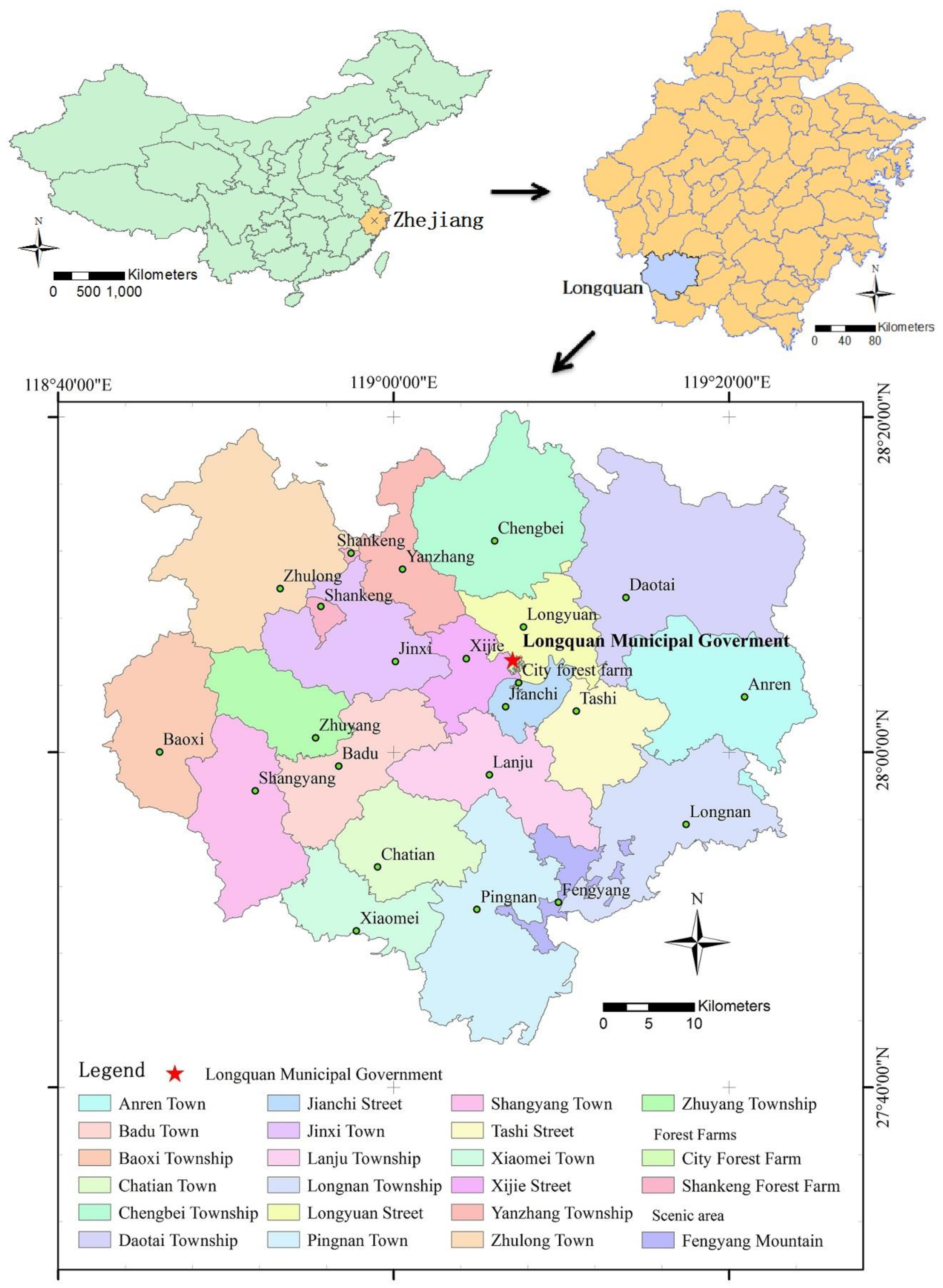
2.1. Study Area
2.2. Evaluation Factors
2.3. Research Data
3. Methods
3.1. Study Scheme Design
3.2. Data Integration
3.3. Evaluation Factors Fitting
3.4. Improved BP Neural Network Model Based on LM Algorithm
- Max_Epochs = 1000
- Input_Num = 17
- Output_Num = 1
- Hidden_Neuron_Num = 2 × Input_Neuron_Num + Output_Neuron_Num
- TransferFcn = {‘tansig’ ‘purelin’}
- TrainFcn = ‘trainlm’
- PerformFcn = ‘mse’
- Net = newff (I, O, Hidden_Neuron_Num)
- [Net TR] = train (Net, I, O)
- Step 4: Prediction.
- y = sim (Net, I_test)
3.5. Model Performance Metrics
4. Results
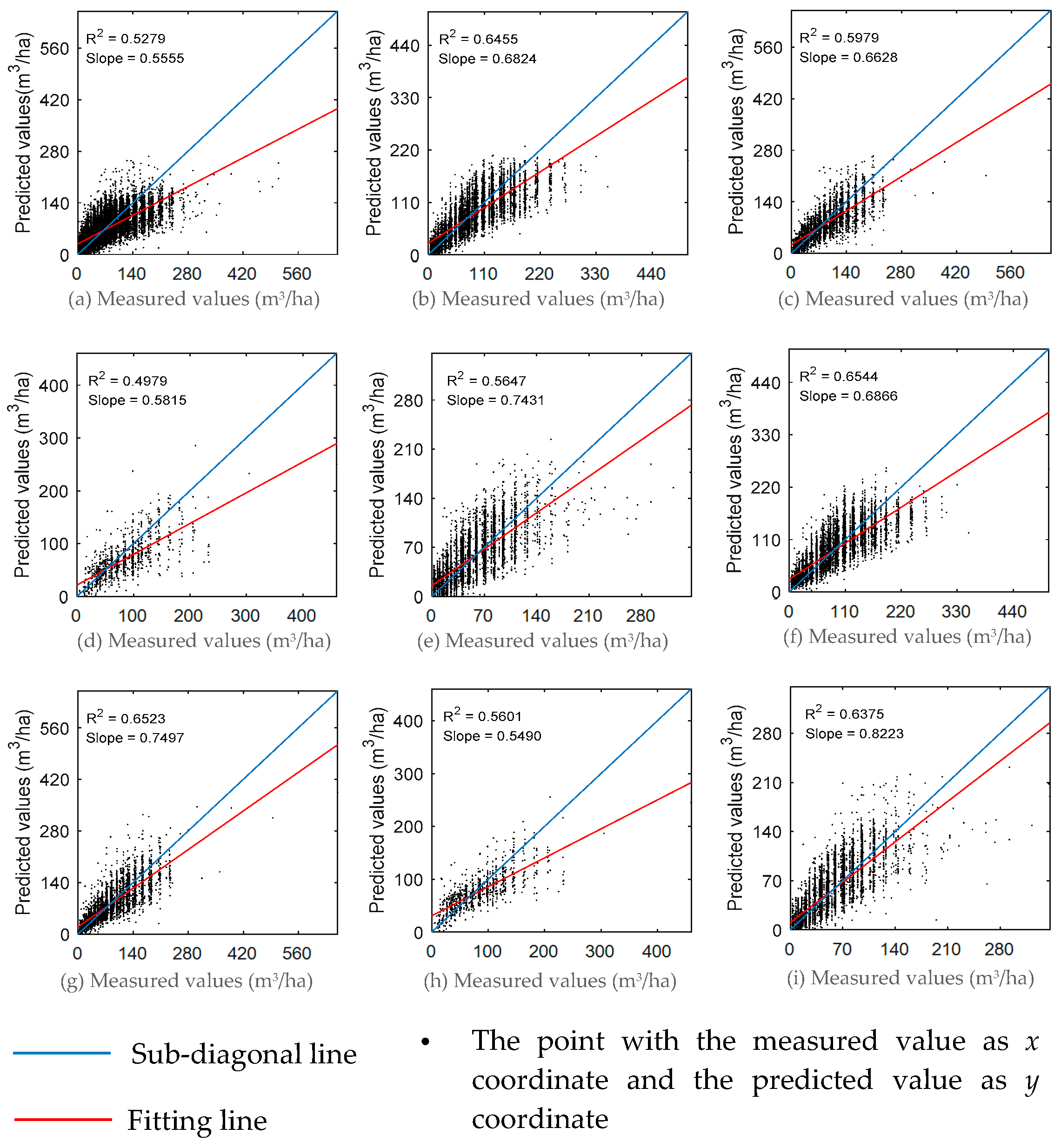
4.1. Modeling
4.2. Predicting
5. Discussion
6. Conclusions
Author Contributions
Funding
Conflicts of Interest
References
- Mohammadi, J.; Joibary, S.S.; Yaghmaee, F.; Mahiny, A.S. Modeling forest stand volume and tree density using Landsat ETM+ data. Int. J. Remote Sens. 2010, 31, 2959–2975. [Google Scholar] [CrossRef]
- Gianfranco, S.; Laura, M.; David, G. Development of a neural network model to update forest distribution data for managed alpine stands. Ecol. Model. 2007, 206, 331–346. [Google Scholar]
- Wu, D.S.; Ji, Y.Q. Dynamic estimation of forest volume based on multi-source data and neural network model. J. Agric. Sci. 2015, 7, 18–31. [Google Scholar] [CrossRef]
- Buckley, D.S.; Isebrands, J.; Sharik, T.L. Practical field methods of estimating canopy cover, PAR, and LAI in Michigan oak and pine stands. North. J. Appl. For. 1999, 16, 25–32. [Google Scholar]
- Chowdhury, T.A.; Thiel, C.; Schmullius, C. Growing stock volume estimation from L-band ALOS PALSAR polarimetric coherence in Siberian forest. Remote Sens. Environ. 2014, 155, 129–144. [Google Scholar] [CrossRef]
- Liu, A.X. Annual Monitoring Theory and Methods of Forest Resources in Zhejiang Province. Ph.D. Thesis, Nanjing Forestry University, Nan Jing, China, June 2006. [Google Scholar]
- Hudak, A.T.; Lefsky, M.A.; Cohen, W.B.; Berterretche, M. Integration of LIDAR and Landsat ETM+ data. Int. Arch. Photogramm. Remote Sens. 2001. [Google Scholar]
- Mäkelä, H.; Pekkarinen, A. Estimation of forest stand volumes by Landsat TM imagery and stand-level field-inventory data. For. Ecol. Manag. 2004, 196, 245–255. [Google Scholar] [CrossRef]
- Shataeea, S.; Weinaker, H.; Babanejad, M. Plot-level forest volume estimation using Airborne Laser Scanner and TM data, comparison of boosting and random forest tree regression algorithms. Procedia Environ. Sci. 2011, 7, 68–73. [Google Scholar] [CrossRef]
- Robinson, A.P.; Monserud, R.A. Criteria for comparing the adaptability of forest growth models. For. Ecol. Manag. 2003, 172, 53–67. [Google Scholar] [CrossRef]
- Mohammadi, Z.; Limaei, S.M.; Lohmander, P.; Olsson, L. Estimation of a basal area growth model for individual trees in uneven-aged Caspian mixed species forests. J. For. Res. 2018, 29, 1205–1214. [Google Scholar] [CrossRef]
- Lamb, S.M.; Maclean, D.A.; Hennigar, C.R.; Pitt, D.G. Forecasting forest inventory using imputed tree lists for LiDAR grid cells and a tree-list growth model. Forests 2018, 9, 167. [Google Scholar] [CrossRef]
- Haykin, S. Neural Networks and Learning Machines, 3rd ed.; Pearson: Upper Saddle River, NJ, USA, 2008. [Google Scholar]
- Castaño-Santamaría, J.; Crecente-Campo, F.; Fernández-Martínez, J.L.; Barrio-Anta, M.; Obeso, J.R. Tree height prediction approaches for uneven-aged beech forests in northwestern Spain. For. Ecol. Manag. 2013, 307, 63–73. [Google Scholar] [CrossRef]
- Wang, S.H.; Zhang, M.Z.; Zhao, P.A.; Chen, J.X. Modelling the spatial distribution of forest carbon stocks with artificial neural network based on TM images and forest inventory data. Acta Ecol. Sin. 2011, 31, 998–1008. [Google Scholar]
- Shataee, S. Non-Parametric Forest Attributes Estimation Using Lidar and TM Data. In Proceedings of the 32nd Asian Conference on Remote Sensing, Taipei, China, 3–7 Octorber 2011; pp. 887–893. [Google Scholar]
- Zhang, D.F. The Design of Neural Network Application based on MATLAB; Machinery Industry Press: Beijing, China, 2009. [Google Scholar]
- Ma, L.; Xu, F.; Wang, X.; Tang, L. Earthquake Prediction Based on Levenberg-Marquardt Algorithm Constrained Back-Propagation Neural Network Using DEMETER Data. In Proceedings of the 4th International Conference on Knowledge Science, Engineering and Management, Belfast, Northern Ireland, UK, 1–3 September 2010; pp. 591–596. [Google Scholar]
- Tomppo, E.; Gschwantner, T.; Lawrence, M.; McRoberts, R.E. National Forest Inventories: Pathways for Common Reporting; Springer: Berlin, Germany, 2010; p. 612. [Google Scholar]
- Debeljaka, M.; Poljanecbk, A.; Ženko, B. Modelling forest growing stock from inventory data: A data mining approach. Ecol. Indic. 2014, 41, 30–39. [Google Scholar] [CrossRef]
- Brown, S.L.; Schroder, P.; Kern, J.S. Spatial distribution of biomass in forests of the eastern USA. For. Ecol. Manag. 1999, 123, 81–90. [Google Scholar] [CrossRef]
- Karjalainen, T.; Nabuurs, G.J.; Eggers, T.; Lapveteläinen, T.; Kaipainen, T. Sce-nario analysis of the impacts of forest management and climate change on the European forest sector carbon budget. For. Policy Econ. 2003, 5, 141–155. [Google Scholar] [CrossRef]
- Franco-Lopeza, H.; Ek, A.R.; Bauer, M.E. Estimation and mapping of forest stand density, volume, and cover type using the k-nearest neighbors method. Remote Sens. Environ. 2001, 77, 251–274. [Google Scholar] [CrossRef] [Green Version]
- Mohammadi, J.; Shataee, S.; Babanezhad, M. Estimation of forest stand volume, tree density and biodiversity using Landsat ETM+ Data, comparison of linear and regression tree analyses. Procedia Environ. Sci. 2011, 7, 299–304. [Google Scholar] [CrossRef]
- McRoberts, R.E.; Gobakken, T.; Næsset, E. Post-stratified estimation of forest area and growing stock volume using lidar-based stratifications. Remote Sens. Environ. 2012, 125, 157–166. [Google Scholar] [CrossRef]
- McRoberts, R.E.; Næsset, E.; Gobakken, T. Inference for Lidar-assisted estimation of forest growing stock volume. Remote Sens. Environ. 2013, 128, 268–275. [Google Scholar] [CrossRef]
- Hong, R.F. Research on the Reform of Foresty Property Rights System in Longquan City. Master’s Thesis, Zhejiang A & F University, Lin’an, China, May 2012. [Google Scholar]
- Zhao, Z. Afforestation Planning and Design Tutorial; China Forestry Press: Beijing, China, 2007. [Google Scholar]
- Deng, L.B.; Li, J.P. Variable density volume prediction model for Chinese fir based on artificial neural network. J. Northwest For. Coll. 2002, 17, 87–89. [Google Scholar]
- Xie, H.Q. Establishment on growth model of Chinese fir and application of multilinear regression. J. Fujian For. Sci. Technol. 2004, 1, 34–37. [Google Scholar]
- Hong, W.; Wu, C.Z.; He, D.J. A study on the model of forest resources management based on the artificial neural network. J. Nat. Res. 1998, 13, 69–72. [Google Scholar]
- Xu, W.M.; Chen, Y.F.; Lin, G.F.; Chen, M.H. Dynamic visualization of Chinese fir volume driven by site condition and growth model. J. Fujian Coll. For. 2011, 31, 151–155. [Google Scholar]
- Lek, S.; Guégan, J.F. Artificial neural networks as a tool in ecological modelling: An introduction. Ecol. Model. 1999, 120, 65–73. [Google Scholar] [CrossRef]
- Li, J.; Cheng, J.H.; Shi, J.Y. Brief introduction of back propagation (BP) neural network algorithm and its improvement. In Advances in Computer Science and Information Engineering; Springer: Berlin/Heidelberg, Germany, 2012; pp. 553–558. [Google Scholar]
- Zheng, C.L.; Jiang, H.Y. K/S value prediction of reactive dyes with improved LM-BP algorithm. J. Text. Res. 2010, 31, 82–85. [Google Scholar]
- Wang, Z.P. Application of LM-BP neural network in lake trophic evaluation. Environ. Sci. Surv. 2013, 32, 98–101. [Google Scholar]
- Hua, Z.; Qian, W.; Gu, L. Application of improved LM-BP neural network in water quality evaluation. Water Resour. Prot. 2008, 24, 22–25. [Google Scholar]
- Jian, X.C.; Wang, L.W.; Min, F. BP neural network based on LM algorithm for the forecasting of vehicle emission. J. Chongqing Univ. Technol. 2012, 26, 11–16. [Google Scholar]
- Miao, X.Y.; Chu, J.K.; Du, X.W. Application of LM-BP neural network in predicting dam deformation. Comput. Eng. Appl. 2011, 47, 220–222. [Google Scholar]
- Gherardo, C.; Anna, B.; Piermaria, C.; Marco, M.; Davide, T.; Fabio, M.; Roberta, B. Non-parametric and parametric methods using satellite images for estimating growing stock volume in Alpine and Mediterranean forest ecosystems. Remote Sens. Environ. 2008, 112, 2686–2700. [Google Scholar]
- Chirici, G.; Corona, P.; Marchetti, M.; Maselli, F.; Bottai, L. Spatial distribution modelling of forest attributes coupling remotely sensed imagery and GIS techniques. In Modelling Forest Systems; Amaro, A., Reed, D., Soares, P., Eds.; CABI Publishing: New York, NY, USA, 2003; pp. 41–50. [Google Scholar]
- Tokola, T.; Heikkila, J. Improving satellite based forest inventory by using a priori site quality information. Silv. Fenn. 1997, 1, 67–78. [Google Scholar] [CrossRef]
- Wu, D.S. Estimation of forest volume based on LM-BP neural network model. Comput. Model. New Technol. 2014, 18, 131–137. [Google Scholar]
- Wei, X.H.; Sun, Y.J.; Ma, W. A height growth model for Cunninghamia lanceolata based on Richards’ equation. J. Zhejiang A & F Univ. 2012, 29, 661–666. [Google Scholar]
- Lin, C.L.; Hong, W.; Wu, C.Z.; He, D.J.; Lan, B. A study on the model of individual accretion of pinusmassoniana forest. J. Fujian Coll. For. 2000, 20, 227–230. [Google Scholar]


| Number | Evaluation Factor | Number | Evaluation Factor |
|---|---|---|---|
| 1 | Tree Age | 2 | Slope |
| 3 | Canopy Density | 4 | Soil Depth |
| 5 | A-layer Depth of Soil | 6 | Aspect |
| 7 | Elevation | 8 | Curvature |
| 9 | Solar Radiation Index | 10 | Topographic Humidity Index |
| 11 | NDVI | 12 | Band 1 |
| 13 | Band 2 | 14 | Band 3 |
| 15 | Band 4 | 16 | Band 5 |
| 17 | Band 7 |
| Group Number | Dominant Tree Species | Number of Subplot | Total Number of Subplot | Proportion (%) |
|---|---|---|---|---|
| Group 1 | Chinese fir | 20,296 | 38,898 | 52.18% |
| Group 2 | Masson pine | 5989 | 15.40% | |
| Group 3 | Taiwan pine | 2418 | 6.22% | |
| Group 4 | Hard broadleaves | 9582 | 24.63% | |
| The other dominant tree species | 613 | 1.58% |
| Number | Dominant Tree Species | Evaluation Factor | Number of Group | Least-Squares Fitting Equation | Correlation Coefficient (R) | Significance (p) |
|---|---|---|---|---|---|---|
| 1 | Chinese fir | Tree Age | 44 | −0.0427890198 × x2 + 6.4914989075 × x + −10.8999069429 | 0.8754 | 0.0000 |
| 2 | Slope | 86 | −0.0115959263 × x2 + 0.6038878174 × x + 82.1824866639 | −0.5336 | 0.0000 | |
| 3 | Aspect | 99 | −0.0033003048 × x2 + 0.4839666164 × x + 72.0559152822 | 0.3246 | 0.0010 | |
| 4 | Elevation | 85 | 0.0023254337 × x2 + −0.2572556056 × x + 89.0182097406 | −0.0945 | 0.3896 | |
| 5 | Curvature | 64 | 0.0065366953 × x2 + −0.5371817451 × x + 90.5614723394 | −0.1003 | 0.4305 | |
| 6 | Solar Radiation Index | 82 | −0.0026200461 × x2 + 0.3467036840 × x + 73.3921706799 | 0.0918 | 0.4120 | |
| 7 | Topographic Humidity Index | 91 | 0.0043653961 × x2 + −0.2512069504 × x + 88.2155051143 | 0.1632 | 0.1221 | |
| 8 | NDVI | 98 | 0.0022565071 × x2 + −0.1541807892 × x + 86.1625587414 | 0.1509 | 0.1380 | |
| 9 | Band 1 | 35 | −0.0118922876 × x2 + 1.5080606424 × x + 43.2161510234 | 0.4637 | 0.0050 | |
| 10 | Band 2 | 22 | −0.0127550587 × x2 + 1.4717083307 × x + 48.6242224527 | 0.3389 | 0.1228 | |
| 11 | Band 3 | 32 | −0.0090806959 × x2 + 0.7815481904 × x + 70.1196285883 | 0.0042 | 0.9818 | |
| 12 | Band 4 | 53 | 0.0020084727 × x2 + −0.0805199224 × x + 84.5622590844 | 0.2199 | 0.1136 | |
| 13 | Band 5 | 80 | −0.0042838563 × x2 + 0.4542927464 × x + 74.8158027009 | 0.0884 | 0.4355 | |
| 14 | Band 7 | 41 | 0.0004892917 × x2 + −0.0031706472 × x + 84.1887249310 | 0.0940 | 0.5586 | |
| 15 | Masson pine | Tree Age | 38 | 0.0331501479 × x2 + 2.8278931378 × x + 15.2328173465 | 0.9482 | 0.0000 |
| 16 | Slope | 78 | −0.0148356773 × x2 + 0.9016394596 × x + 67.9666405506 | −0.3331 | 0.0029 | |
| 17 | Aspect | 94 | −0.0032729759 × x2 + 0.2348500208 × x + 75.6303889833 | −0.1668 | 0.1081 | |
| 18 | Elevation | 70 | −0.0206467958 × x2 + 1.1473753074 × x + 65.8295224974 | −0.4560 | 0.0001 | |
| 19 | Curvature | 47 | −0.0065277438 × x2 + 0.3054885854 × x + 74.8842350529 | −0.0234 | 0.8758 | |
| 20 | Solar Radiation Index | 67 | −0.0116390188 × x2 + 1.7344282575 × x + 16.7808352190 | 0.5074 | 0.0000 | |
| 21 | Topographic Humidity Index | 79 | 0.0068459173 × x2 + −0.6174814023 × x + 82.0851684875 | 0.0086 | 0.9402 | |
| 22 | NDVI | 90 | 0.0040823038 × x2 + −0.1607289597 × x + 72.4870953181 | 0.2413 | 0.0220 | |
| 23 | Band 1 | 30 | 0.0215449663 × x2 + −1.4478075547 × x + 83.4298332936 | 0.4954 | 0.0054 | |
| 24 | Band 2 | 19 | −0.0107774671 × x2 + 1.1612851686 × x + 43.9676859378 | 0.1036 | 0.6731 | |
| 25 | Band 3 | 28 | −0.0056810995 × x2 + 0.6748729435 × x + 57.9892594691 | 0.1594 | 0.4178 | |
| 26 | Band 4 | 49 | 0.0051865652 × x2 + −0.4677663146 × x + 83.9501363669 | 0.0103 | 0.9442 | |
| 27 | Band 5 | 72 | 0.0010562299 × x2 + −0.2748031246 × x + 86.6400382977 | −0.1567 | 0.1888 | |
| 28 | Band 7 | 39 | 0.0121557341 × x2 + −0.9500200238 × x + 83.6278316688 | 0.1422 | 0.3880 | |
| 29 | Taiwan pine | Tree Age | 46 | 0.0108691950 × x2 + 2.8041406197 × x + 0.7548379420 | 0.9153 | 0.0000 |
| 30 | Slope | 71 | 0.0007210346 × x2 + −0.1981166266 × x+80.5153065313 | −0.0985 | 0.4140 | |
| 31 | Aspect | 92 | −0.0033269117 × x2 + 0.4194282364 × x + 62.0507244967 | 0.1330 | 0.2064 | |
| 32 | Elevation | 67 | −0.0170165295 × x2 + 2.0442044776 × x + 13.8462032002 | 0.1801 | 0.1447 | |
| 33 | Curvature | 52 | −0.0089471129 × x2 + 0.1602318306 × x + 74.2890687778 | −0.2853 | 0.0404 | |
| 34 | Solar Radiation Index | 77 | 0.0024392679 × x2 + −0.1965197674 × x + 72.5025712358 | 0.1011 | 0.3816 | |
| 35 | Topographic Humidity Index | 33 | −0.0162849784 × x2 + 1.1347361067 × x + 56.4756479999 | 0.0568 | 0.7537 | |
| 36 | NDVI | 85 | −0.0018733247 × x2 + 0.3472925064 × x + 60.4853464235 | 0.2063 | 0.0581 | |
| 37 | Band 1 | 15 | 0.0584268211 × x2 + −2.8925728373 × x + 102.4213645020 | 0.1372 | 0.6259 | |
| 38 | Band 2 | 11 | 0.0462181612 × x2 + −2.0249896794 × x + 87.1407802797 | 0.4339 | 0.1824 | |
| 39 | Band 3 | 17 | 0.0520556446 × x2 + −1.8273924977 × x + 82.6589015604 | 0.3448 | 0.1753 | |
| 40 | Band 4 | 45 | −0.0026199728 × x2 + 0.2061151757 × x + 69.9711400898 | −0.0155 | 0.9195 | |
| 41 | Band 5 | 63 | 0.0012177555 × x2 + −0.1554842686 × x + 74.2397400623 | −0.0815 | 0.5255 | |
| 42 | Band 7 | 32 | 0.0142484577 × x2 + −0.6341009191 × x + 75.5528181515 | 0.3688 | 0.0378 | |
| 43 | Hard broadleaves | Tree Age | 62 | 0.0163003073 × x2 + 1.1534510399 × x + 17.1575498742 | 0.9163 | 0.0000 |
| 44 | Slope | 85 | 0.0036011768 × x2 + −0.6254997771 × x + 74.8775043187 | −0.3450 | 0.0012 | |
| 45 | Aspect | 96 | 0.0039735998 × x2 + −0.3577728963 × x + 58.2501579702 | 0.0960 | 0.3520 | |
| 46 | Elevation | 83 | 0.0180034120 × x2 + −1.3930520666 × x + 71.4995888064 | 0.1853 | 0.0935 | |
| 47 | Curvature | 60 | 0.0286950221 × x2 + −1.5689644141 × x + 64.8735422419 | 0.1606 | 0.2203 | |
| 48 | Solar Radiation Index | 87 | 0.0040370576 × x2 + −0.2975027144 × x + 55.5262852886 | 0.1829 | 0.0900 | |
| 49 | Topographic Humidity Index | 62 | 0.0277373791 × x2 + −1.8961270968 × x + 72.8165360650 | 0.2434 | 0.0566 | |
| 50 | NDVI | 93 | −0.0027252454 × x2 + 0.2307572964 × x + 48.9924512551 | −0.0468 | 0.6558 | |
| 51 | Band 1 | 29 | 0.0626190912 × x2 + −4.5932489190 × x + 123.0293545383 | 0.3439 | 0.0678 | |
| 52 | Band 2 | 18 | 0.0292226631 × x2 + −2.1099893402 × x + 81.3753529658 | 0.5453 | 0.0192 | |
| 53 | Band 3 | 28 | 0.0226705539 × x2 + −1.2930119073 × x + 66.0857518410 | 0.4885 | 0.0084 | |
| 54 | Band 4 | 52 | 0.0029985089 × x2 + −0.4153878341 × x + 62.4330118645 | −0.2118 | 0.1317 | |
| 55 | Band 5 | 69 | 0.0133684136 × x2 + −0.9407788330 × x + 62.4965426573 | 0.1885 | 0.1210 | |
| 56 | Band 7 | 33 | 0.0297143535 × x2 + −1.7693736017 × x + 67.6223561210 | 0.3281 | 0.0623 |
| Scheme | Dominant Tree Species | Numbers of Sample | Average Measured Value (m3) | Average Predicted Value (m3) | GAPE (%) | MAPE (%) | MAE (m3) | RMSE (m3) | IA | R2 |
|---|---|---|---|---|---|---|---|---|---|---|
| Scheme 1 | Mixed | 16112 | 76.8375 | 75.2040 | 2.1251 | 41.0680 | 20.4495 | 28.119 | 0.8773 | 0.6388 |
| Scheme 2 | Chinese fir | 9529 | 85.0350 | 83.4120 | 1.9097 | 29.4761 | 18.0450 | 24.6525 | 0.9117 | 0.7212 |
| Masson pine | 1872 | 79.1520 | 76.2300 | 3.6916 | 30.1500 | 18.1140 | 23.9415 | 0.9080 | 0.7107 | |
| Taiwan pine | 1457 | 70.5510 | 66.8235 | 5.2822 | 25.0961 | 14.9265 | 20.4195 | 0.9276 | 0.7605 | |
| Hard broadleaves | 3014 | 54.5385 | 54.3390 | 0.3673 | 44.5836 | 14.9295 | 21.5490 | 0.9181 | 0.7372 | |
| Scheme 3 | Chinese fir | 9529 | 85.0354 | 86.0979 | 1.2495 | 31.3399 | 18.3058 | 25.0376 | 0.9087 | 0.7116 |
| Masson pine | 1872 | 79.1524 | 79.9650 | 1.0267 | 31.4837 | 18.4711 | 24.4194 | 0.9041 | 0.6949 | |
| Taiwan pine | 1457 | 70.5505 | 70.4016 | 0.2110 | 27.2093 | 15.4221 | 21.4346 | 0.9153 | 0.7261 | |
| Hard broadleaves | 3014 | 54.5391 | 54.2795 | 0.4760 | 45.3362 | 15.6780 | 23.0508 | 0.9049 | 0.6991 |
| Modeling or Predicting | Scheme Name | Number of Sample | Average Measured Value (m3) | Average Predicted Value (m3) | GAPE (%) | MAPE (%) | MAE (m3) | RMSE (m3) | IA | R2 |
|---|---|---|---|---|---|---|---|---|---|---|
| Modeling | Scheme 1 | 16,112 | 76.8375 | 75.2040 | 2.1251 | 41.0680 | 20.4495 | 28.1190 | 0.8773 | 0.6388 |
| Scheme 2 | 15,872 | 77.2215 | 75.5205 | 2.2011 | 32.0223 | 17.1750 | 23.6415 | 0.9202 | 0.7427 | |
| Scheme 3 | 15,872 | 77.2215 | 77.8916 | 0.8687 | 33.6355 | 17.5616 | 24.2850 | 0.9157 | 0.7272 | |
| Predicting | Scheme 1 | 22,786 | 72.8010 | 69.3690 | 4.7149 | 50.2675 | 24.1500 | 33.6555 | 0.8296 | 0.5279 |
| Scheme 2 | 22,413 | 73.2135 | 71.2950 | 2.6217 | 41.7724 | 20.9190 | 28.9950 | 0.8883 | 0.6460 | |
| Scheme 3 | 22,413 | 73.2135 | 73.3415 | 0.1739 | 37.5268 | 19.5685 | 27.4908 | 0.9036 | 0.6823 |
| Scheme | Dominant Tree Species | Number of Sample | Average Measured Value (m3) | Average Predicted Value (m3) | GAPE (%) | MAPE (%) | MAE (m3) | RMSE (m3) | IA | R2 |
|---|---|---|---|---|---|---|---|---|---|---|
| Scheme 1 | Mixed | 22,786 | 72.8010 | 69.3690 | 4.7149 | 50.2675 | 24.1500 | 33.6555 | 0.8296 | 0.5279 |
| Scheme 2 | Chinese fir | 10,767 | 83.0250 | 80.9520 | 2.4971 | 31.5641 | 20.8275 | 28.6515 | 0.8862 | 0.6455 |
| Masson pine | 4117 | 87.3510 | 80.2590 | 8.1192 | 37.8890 | 24.6330 | 34.0260 | 0.8657 | 0.5979 | |
| Taiwan pine | 961 | 82.4640 | 69.6090 | 15.5888 | 35.9952 | 25.5375 | 36.1290 | 0.8105 | 0.4979 | |
| Hard broadleaves | 6568 | 46.9170 | 50.0910 | 6.7675 | 61.7867 | 18.0675 | 24.6255 | 0.8604 | 0.5647 | |
| Scheme 3 | Chinese fir | 10,767 | 83.0250 | 83.6362 | 0.7361 | 32.8997 | 20.3668 | 28.2005 | 0.8897 | 0.6544 |
| Masson pine | 4117 | 87.3510 | 84.8161 | 2.9019 | 34.4703 | 22.5600 | 31.4144 | 0.8942 | 0.6523 | |
| Taiwan pine | 961 | 82.4640 | 76.0733 | 7.7503 | 35.4529 | 22.6440 | 31.8299 | 0.8332 | 0.5601 | |
| Hard broadleaves | 6568 | 46.9170 | 48.8730 | 4.1704 | 47.3315 | 15.9346 | 22.5483 | 0.8893 | 0.6375 |
© 2018 by the authors. Licensee MDPI, Basel, Switzerland. This article is an open access article distributed under the terms and conditions of the Creative Commons Attribution (CC BY) license (http://creativecommons.org/licenses/by/4.0/).
Share and Cite
Zhou, R.; Wu, D.; Fang, L.; Xu, A.; Lou, X. A Levenberg–Marquardt Backpropagation Neural Network for Predicting Forest Growing Stock Based on the Least-Squares Equation Fitting Parameters. Forests 2018, 9, 757. https://doi.org/10.3390/f9120757
Zhou R, Wu D, Fang L, Xu A, Lou X. A Levenberg–Marquardt Backpropagation Neural Network for Predicting Forest Growing Stock Based on the Least-Squares Equation Fitting Parameters. Forests. 2018; 9(12):757. https://doi.org/10.3390/f9120757
Chicago/Turabian StyleZhou, Ruyi, Dasheng Wu, Luming Fang, Aijun Xu, and Xiongwei Lou. 2018. "A Levenberg–Marquardt Backpropagation Neural Network for Predicting Forest Growing Stock Based on the Least-Squares Equation Fitting Parameters" Forests 9, no. 12: 757. https://doi.org/10.3390/f9120757